A Stochastic Evolutionary Model Exhibiting Power-Law Behaviour with an Exponential Cutoff

Abstract

Recently several authors have proposed stochastic evolutionary models for the growth of complex networks that give rise to power-law distributions. These models are based on the notion of preferential attachment leading to the “rich get richer” phenomenon. Despite the generality of the proposed stochastic models, there are still some unexplained phenomena, which may arise due to the limited size of networks such as protein and e-mail networks. Such networks may in fact exhibit an exponential cutoff in the power-law scaling, although this cutoff may only be observable in the tail of the distribution for extremely large networks. We propose a modification of the basic stochastic evolutionary model, so that after a node is chosen preferentially, say according to the number of its inlinks, there is a small probability that this node will be discarded. We show that as a result of this modification, by viewing the stochastic process in terms of an urn transfer model, we obtain a power-law distribution with an exponential cutoff. Unlike many other models, the current model can capture instances where the exponent of the distribution is less than or equal to two. As a proof of concept, we demonstrate the consistency of our model by analysing a yeast protein interaction network, the distribution of which is known to follow a power law with an exponential cutoff.

1 Introduction

Power-law distributions taking the form

$$f(i)=C\ i^{-\tau},$$ (1)

where $C$ and $\tau$ are positive constants, are abundant in nature [Sor00]. The constant $\tau$ is called the exponent of the distribution. Examples of such distributions are: Zipf’s law, which states that the relative frequency of words in a text is inversely proportional to their rank, Pareto’s law, which states that the number of people whose personal income is above a certain level follows a power-law distribution with an exponent between 1.5 and 2 (Pareto’s law is also known as the 80:20 law, stating that about 20% of the population earn 80% of the income) and Gutenberg-Richter’s law, which states that, over a period of time, the number of earthquakes of a certain magnitude is roughly inversely proportional to the magnitude. Recently, several researchers have detected power-law distributions in the topology of various networks such as the World-Wide-Web [BKM⁺00, KRR⁺00] and author citation graphs [Red98].

The motivation for the current research is two-fold. First, from a complex network perspective, we would like to understand the stochastic mechanisms that govern the growth of a network. This has lead to fruitful interdisciplinary research by a mixture of Computer Scientists, Mathematicians, Statisticians, Physicists, and Social Scientists [AB02, DM00, KRL00, New01, PFL⁺02], who are actively involved in investigating various characteristics of complex networks, such as the degree distribution of the nodes, the diameter, and the relative sizes of various components. These researchers have proposed several stochastic models for the evolution of complex networks; all of these have the common theme of preferential attachment — which results in the “rich get richer” phenomenon — for example, where new links to existing nodes are added in proportion to the number of links to these nodes currently present. Considering the web as an example of a complex network, one of the challenges in this line of research is to explain the empirically discovered power-law distributions [AH01]. It turns out that the evolutionary model of preferential attachment fails to explain several of the empirical results, due to the fact that the exponents predicted are inconsistent with the observations. To address this problem, we proposed in [LFLW02] an extension of the stochastic model for the web’s evolution in which the addition of links utilises a mixture of preferential and non-preferential mechanisms. We introduced a general stochastic model involving the transfer of balls between urns that also naturally models quantities such as the numbers of web pages in and visitors to a web site, which are not naturally described in graph-theoretic terms.

Another extension of the preferential attachment model, proposed in [DM00], takes into account the ageing of nodes, so that a link is connected to an old node, not only preferentially, but also depending on the age of the node: the older the node is, the less likely it is that other nodes will be connected to it. It was shown in [DM00] that if the ageing function is a power law then the degree distribution has a phase transition from a power-law distribution, when the exponent of the ageing function is less than one, to an exponential distribution, when the exponent is greater than one. A different model of node ageing was proposed in [ASBS00] with two alternative ageing functions. With the first function the time a node remains ‘active’, i.e. may acquire new links, decays exponentially, and with the second function a node remains active until it has acquired a maximum number of links. Both functions were shown by simulation to lead to an exponential cutoff in the degree distribution, and for strong enough constraints the distribution appeared to be purely exponential. Another explanation for a cutoff, offered in [MBSA02], is that when a link is created the author of the link has limited information processing capabilities and thus only considers linking to a fraction of the existing nodes, those that appear to be “interesting”. It was shown by simulation that when the fraction of “interesting nodes” is less than one there is a change from a power-law distribution to one that exhibits an exponential cutoff, leading eventually to an exponential distribution when the fraction is much less than one.

A second motivation for this research is that the viability and efficiency of network algorithmics are affected by the statistical distributions that govern the network’s structure. For example, the discovered power-law distributions in the web have recently found applications in local search strategies in web graphs [ALPH01], compression of web graphs [AM01] and an analysis of the robustness of networks against error and attack [AJB00, JMBO01].

Despite the generality of the proposed stochastic models for the evolution of complex networks, there are still some unexplained phenomena; these may arise due to the limited size of networks such as protein, e-mail, actor and collaboration networks. Such networks may in fact exhibit an exponential cutoff in the power-law scaling, although this cutoff may only be observable in the tail of the distribution for extremely large networks. The exponential cutoff is of the form

$$f(i)=C\ i^{-\tau}q^{i},$$ (2)

with $0<q<1$. The exponent $\tau$ in (2) will be smaller than the exponent that would be obtained if we tried to fit a power law without a cutoff, like (1), to the data. Unlike many other models leading to power-law distributions, models with a cutoff can capture situations in which the exponent of the distribution is less than or equal to two, which would otherwise have infinite expectation.

An exponential cutoff has been observed in protein networks [JMBO01], in e-mail networks [EMB02], in actor networks [ASBS00], in collaboration networks [New01, Gro02], and is apparently also present in the distribution of inlinks in the web graph [MBSA02], where a cutoff had not previously been observed. We believe it is likely, in many such cases where power-law distributions have been observed, that better models would be obtained with an exponential cutoff like (2), with $q$ very close to one.

The main aim of this paper is to provide a stochastic evolutionary model that results in asymptotic power-law distributions with an exponential cutoff, thus allowing us to model discrete finite systems more accurately and, in addition, enabling us to explain phenomena where the exponent is less than or equal to two. As with many of these stochastic growth models, the ideas originated from Simon’s visionary paper published in 1955 [Sim55]. At the very beginning of his paper, in equation (1.1), Simon observed that the class of distribution functions he was about to analyse can be approximated by a distribution like (2); he called the term $q^{i}$ the convergence factor and suggested that $q$ is close to one. He then went on to present his well-known model that yields power-law distributions like (1), and which has provided the basis for the models rediscovered over 40 years later. Simon gave no explanation for the appearance, in practice, of the convergence factor.

Considering, for example, the web graph, the modification we make to the basic model to explain the convergence factor is that after a web page is chosen preferentially, say according to the number of its inlinks, there is a small probability that this page will be discarded. A possible reason for this may be that the web page has acquired too many inlinks and therefore needs to be redesigned, or simply that an error has occurred and the page is lost. Other examples are e-mail networks, where new users join and old users leave the network, and protein networks, where proteins may appear or disappear from the network over time.

Networks with an exponential cutoff fall into two categories. The first category of network, which includes actor and collaboration networks, is monotonically increasing, i.e. nodes and links are never removed from such networks. In this category nodes can be either active, in which case they can be the source or destinations of new links, or inactive in which case they are not involved in any new links from the time they first become inactive. The second category of network, which includes the web graph, e-mail and protein networks, is non-monotonic, i.e. links and nodes may be removed. In this paper we consider the second category of network, but only allow node deletion. (In [FLL05] we considered the case where only link removal is allowed and showed that in that case the degree distribution follows a power law.) The first category of network (which also exhibits an exponential cutoff in the degree distribution) will be dealt with in a follow-up paper.

The rest of the paper is organised as follows. In Section 2 we present an urn transfer model that extends Simon’s model by allowing a ball to sometimes be discarded. In Section 3 we derive the steady state distribution of the model, which, as stated, follows an asymptotic power law with an exponential cutoff like (2). In Section 4 we demonstrate that our model can provide an explanation of the empirical distributions found in protein networks. Finally, in Section 5 we give our concluding remarks.

2 An Urn Transfer Model

We now present an urn transfer model [JK77] for a stochastic process that emulates the situation when balls (which might represent, for example, proteins or email accounts) are discarded with a small probability. This model can be viewed as an extension of Simon’s model [Sim55], where either a ball is added to the first urn with probability $p$, or some ball is moved along from the urn it is in to the next urn with probability $1-p$. We assume that a ball in the $i$th urn has $i$ pins attached to it (which might represent, for example, interactions between proteins or e-mail messages between email accounts). We note that there is a correspondence between the Barabási and Albert model [BA99], defined in terms of nodes and links, and Simon’s model, defined in terms of balls and pins, as was established in [BE01]. Essentially, the correspondence is obtained by noting that the balls in an urn can be viewed as an equivalence class of nodes all having the same connectivity (i.e. degree).

We assume a countable number of urns, $urn_{1},urn_{2},urn_{3},\ldots\$. Initially all the urns are empty except $urn_{1}$, which has one ball in it. Let $F_{i}(k)$ be the number of balls in $urn_{i}$ at stage $k$ of the stochastic process, so $F_{1}(1)=1$ and all other $F_{i}(1)=0$. Then, at stage $k+1$ of the stochastic process, where $k\geq 1$, one of two things may occur:

1. with probability $p$, $0<p<1$, a new ball (with one pin attached) is inserted into $urn_{1}$, or

2. with probability $1-p$ an urn is selected, with $urn_{i}$ being selected with probability proportional to $iF_{i}(k)$ (i.e. $urn_{i}$ is selected preferentially in proportion to the total number of pins it contains), and a ball is chosen from the selected urn, $urn_{i}$ say; then,

   1. with probability $q$, $0<q\leq 1$, the chosen ball is transferred to $urn_{i+1}$, (this is equivalent to attaching an additional pin to the ball chosen from $urn_{i}$), or

   2. with probability $1-q$ the ball chosen is discarded.

The expected total number of balls in the urns at stage $k$ is given by

$$E\Big{(}\sum_{i=1}^{k}F_{i}(k)\Big{)} = 1+(k-1)\Big{(}p-(1-p)(1-q)\Big{)}$$ (3)

$$= (1-p)(2-q)+k\Big{(}p-(1-p)(1-q)\Big{)}.$$

We note that we could modify the initial conditions so that, for example, $urn_{1}$ initially contained $\delta>1$ balls instead of one. It can be shown, from the development of the model below, that any change in the initial conditions will have no effect on the asymptotic distribution of the balls in the urns as $k$ tends to infinity, provided the process does not terminate with all of the urns empty.

To ensure that, on average, more balls are added to the system than are discarded, on account of (3) we require $p>(1-p)(1-q)$, which implies

$$q>\frac{1-2p}{1-p};$$

this trivially holds for $p>1/2$.

From now on we assume that this holds. This constraint implies that the probability that the urn transfer process will not terminate with all the urns being empty is positive. More specifically, the probability of non-termination is given by

$$1-\left(\frac{(1-p)(1-q)}{p}\right)^{\delta},$$ (4)

where $\delta$ is the initial number of balls in $urn_{1}$; this is exactly the probability that the gambler’s fortune will increase forever [Ros83].

The total number of pins attached to balls in $urn_{i}$ at stage $k$ is $iF_{i}(k)$, so the expected total number of pins in the urns is given by

$$E\Big{(}\sum_{i=1}^{k}iF_{i}(k)\Big{)} = 1+(k-1)\Big{(}p+(1-p)q\Big{)}-(1-p)(1-q)\sum_{j=1}^{k-1}\theta_{j}$$ (5)

$$= k\Big{(}p+(1-p)q\Big{)}-(1-p)(1-q)\Big{(}\sum_{j=1}^{k-1}\theta_{j}-1\Big{)},$$

where $\theta_{j}$, $1\leq j\leq k-1$, is the expectation of $\Theta_{j}$, the number of pins attached to the ball chosen at step (ii) of stage $j$ (i.e. the urn number). So

$$\theta_{j}=E(\Theta_{j})=E\left(\frac{\sum_{i=1}^{j}i^{2}F_{i}(j)}{\sum_{i=1}^{j}iF_{i}(j)}\right).$$ (6)

As a consequence we have

$$1\leq\theta_{j}\leq j,$$

since at stage $j$ there cannot be more than $j$ pins in the system.

Now let

$$\theta^{(k)}=\frac{1}{k}\sum_{j=1}^{k}\theta_{j}.$$

Since there are at least as many pins in the system as there are balls, it follows from (3) and (5) that

$$1\leq\theta^{(k)}\leq\frac{1}{1-q}.$$ (7)

So, since $\theta^{(k)}$ is bounded, we will make the reasonable assumption that $\theta^{(k)}$ tends to a limit $\theta$ as $k$ tends to infinity, i.e.

$$\lim_{k\to\infty}\theta^{(k)}=\theta.$$

Letting $k$ tend to infinity in (7) gives

$$1\leq\theta\leq\frac{1}{1-q}.$$

In the next section we demonstrate through simulation of the stochastic process that our assumption that $\theta^{(k)}$ converges appears to hold. We also explain how the asymptotic value $\theta$ may be obtained, assuming that the limit exists.

3 Derivation of the Steady State Distribution

Following Simon [Sim55], we now state the mean-field equations for the urn transfer model. For $i>1$ we have

$$E_{k}(F_{i}(k+1))=F_{i}(k)+\beta_{k}\Big{(}q(i-1)F_{i-1}(k)-iF_{i}(k)\Big{)},$$ (8)

where $E_{k}(F_{i}(k+1))$ is the expected value of $F_{i}(k+1)$ given the state of the model at stage $k$, and

$$\beta_{k}=\frac{1-p}{\sum_{i=1}^{k}\ iF_{i}(k)}$$ (9)

is the normalising factor.

Equation (8) gives the expected number of balls in $urn_{i}$ at stage $k+1$. This is equal to the previous number of balls in $urn_{i}$ plus the probability of adding a ball to $urn_{i}$ minus the probability of removing a ball from $urn_{i}$. The former probability is just the probability of choosing a ball from $urn_{i-1}$ and transferring it to $urn_{i}$ in step (ii)(a) of the stochastic process defined in Section 2, whilst the latter probability is the probability of choosing a ball from $urn_{i}$ in step (ii) of the process.

In the boundary case, $i=1$, we have

$$E_{k}(F_{1}(k+1))=F_{1}(k)+p-\beta_{k}\ F_{1}(k),$$ (10)

for the expected number of balls in $urn_{1}$, which is equal to the previous number of balls in the first urn plus the probability of inserting a new ball into $urn_{1}$ in step (i) of the stochastic process defined in Section 2 minus the probability of choosing a ball from $urn_{1}$ in step (ii).

In order to solve the equations for the model, we make the assumption that, for large $k$, the random variable $\beta_{k}$ can be approximated by a constant (i.e. non-random) value depending only on $k$. We take this approximation to be

$$\hat{\beta}_{k}=\frac{1-p}{k\left(p+(1-p)q-(1-p)(1-q)\theta^{(k)}\right)}.$$

The motivation for this approximation is that the denominator in the definition of $\beta_{k}$ has been replaced by an asymptotic approximation of its expectation as given in (5). We observe that replacing $\beta_{k}$ by $\hat{\beta}_{k}$ results in an approximation similar to that of the “$p_{k}$ model” in [LFLW02], which is essentially a mean-field approach.

We can now take expectations of (8) and (10). Thus, by the linearity of the expectation operator $E(.)$, we obtain

$$E(F_{i}(k+1))=E(F_{i}(k))+\hat{\beta}_{k}\Big{(}q(i-1)E(F_{i-1}(k))-iE(F_{i}(k))\Big{)}$$ (11)

and

$$E(F_{1}(k+1))=E(F_{1}(k))+p-\hat{\beta}_{k}E(F_{1}(k)).$$ (12)

In order to obtain an asymptotic solution of equations (11) and (12), we require that $E(F_{i}(k))/k$ converges to $f_{i}$ as $k$ tends to infinity. Suppose for the moment that this is the case, then, provided the convergence is fast enough, $E(F_{i}(k+1))-E(F_{i}(k))$ tends to $f_{i}$. By “fast enough” we mean $\epsilon_{i,k+1}-\epsilon_{i,k}$ is $o(1/k)$ for large $k$, where

$$E(F_{i}(k))=k(f_{i}+\epsilon_{i,k}).$$

Now, letting

$$\beta=\frac{1-p}{p+(1-p)q-(1-p)(1-q)\theta},$$ (13)

we see that $\hat{\beta_{k}}E(F_{i}(k))$ tends to $\beta f_{i}$ as $k$ tends to infinity.

So, letting $k$ tend to infinity, (11) and (12) yield

$$f_{i}=\beta\Big{(}q(i-1)f_{i-1}-if_{i}\Big{)},$$ (14)

for $i>1$, and

$$f_{1}=p-\beta f_{1}.$$ (15)

Following the lines of the proof given in the Appendix of [LFLW02], we can show that $\epsilon_{i,k}$ tends to zero as $k$ tends to infinity provided we make the further assumption that

$$\mid\!\theta-\theta^{(k)}\!\mid\leq\frac{c}{k},$$

for some constant $c$. In other words, this assumption states that the expected number of pins attached to the balls chosen in the first $k$ stages of the stochastic process is within a constant of the asymptotic expected number of pins attached to the chosen ball multiplied by $k$, i.e.

$$k\theta-c\leq\sum_{j=1}^{k}\theta_{j}\leq k\theta+c.$$

In order to verify the convergence we ran some simulations; these will be discussed at the end of this section.

Provided that $\beta_{k}$ can be approximated by $\hat{\beta}_{k}$ for large $k$, then, under the stated assumptions, $f_{i}$ is the asymptotic expected rate of increase of the number of balls in $urn_{i}$; thus the asymptotic proportion of balls in $urn_{i}$ is proportional to $f_{i}$.

From (14) and (15) we obtain

$$f_{i}=\frac{\beta\ q\ (i-1)}{1+i\beta}\ f_{i-1}=\frac{q\ (i-1)}{i+\varrho}\ f_{i-1}$$ (16)

and

$$f_{1}=\frac{p}{1+\beta}=\frac{\varrho\ p}{1+\varrho},$$ (17)

where $\varrho=1/\beta$. Now, on repeatedly using (16), we get

$$f_{i}=\frac{\varrho\ p\ q^{i-1}\ 1\ 2\ \cdots\ (i-1)}{(1+\varrho)\ (2+\varrho)\ \cdots\ (i+\varrho)}=\frac{\varrho\ p\ \Gamma(1+\varrho)\ \Gamma(i)\ q^{i}}{q\ \Gamma(i+1+\varrho)},$$ (18)

where $\Gamma$ is the gamma function [AS72, 6.1].

Thus for large $i$, on using Stirling’s approximation [AS72, 6.1.39], we obtain $f_{i}$ in a form corresponding to (2):

$$f_{i}\sim\frac{C\ q^{i}}{i^{1+\varrho}},$$ (19)

where $\sim$ means is asymptotic to, and

$$C=\frac{\varrho\ p\ \Gamma(1+\varrho)}{q}.$$

From (18), it follows that

$$\sum_{i=1}^{\infty}f_{i} = \frac{\varrho\ p\ \Gamma(2+\varrho)}{1+\varrho}\ \sum_{j=0}^{\infty}\frac{\Gamma(j+1)\ \Gamma(j+1)}{\Gamma(j+2+\varrho)}\frac{q^{j}}{j!}$$ (20)

$$= \frac{\varrho\ p}{1+\varrho}\ F(1,1;2+\varrho;q),$$

where $F$ is the hypergeometric function [AS72, 15.1.1]. From (20) it is immediate that the first moment is given by

$$\sum_{i=1}^{\infty}if_{i}=\frac{\varrho\ p}{1+\varrho}\ F(1,2;2+\varrho;q),$$ (21)

and the second moment is given by

$$\sum_{i=1}^{\infty}i^{2}f_{i}=\frac{\varrho\ p}{1+\varrho}\ F(2,2;2+\varrho;q).$$ (22)

Under the assumptions we have made for the steady state distribution, using (6), (21) and (22) we obtain

$$\theta=\frac{F(2,2;2+\varrho;q)}{F(1,2;2+\varrho;q)}.$$ (23)

In the special case when $q=1$, which is Simon’s original model, using the fact that in this case $\varrho=1/(1-p)$, we obtain by Gauss’s formula [AS72, 15.1.20]

$$\sum_{i=1}^{\infty}if_{i}=1,$$

as expected, and

$$\sum_{i=1}^{\infty}i^{2}f_{i}=\frac{1}{2p-1},$$

which is valid only if $p>0.5$, i.e. $\varrho>2$.

Letting $k$ tend to infinity in (5) and using (13) we obtain

$$\sum_{i=1}^{\infty}if_{i}=\frac{1-p}{\beta}=\varrho(1-p).$$

Together with (21), this gives the following equation for $\varrho$ in terms of $p$ and $q$:

$$(1-p)(1+\varrho)=p\ F(1,2;2+\varrho;q).$$ (24)

This equation may be solved numerically to obtain the value of $\varrho$, and $\theta$ can then be obtained from (13) or (23). (It can be shown that, by virtue of (24), both equations yield the same value for $\theta$.)

In order to verify the convergence assumptions we ran several stochastic simulations. For $p=0.3$ and $q=0.975$, the number of aborts (i.e. computations terminating because all the urns were empty) predicted by (4) is about 5.8%. We ran the simulations 1000 times, each run for 1000 steps. There were 49 aborts, with the maximum number of steps before aborting being 12 and the average 4.14.

Figure 1 shows a summary of ten runs, each of half a million steps, with the above parameters, plotting $\Theta_{j}$ against $j$. The bottom plot is the minimum $\Theta_{j}$ over the ten runs, the middle plot is the average and the top plot is the maximum. The asymptotic average value of $\Theta_{j}$ was $11.1902$. On the other hand, computing $\theta$ from (23), averaged over ten runs, with $\varrho$ taken to be $(k\beta_{k})^{-1}$, gave 11.1762. As a final check, computing $\varrho$ from (24) and $\theta$ from (23) or (13) gives 11.1753. In further simulations, similar plots were obtained for other values of $p$ and $q$.

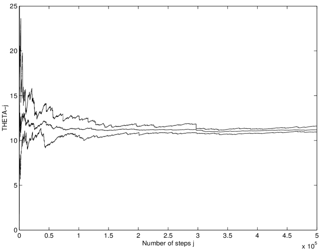
Figure 1: Convergence of $\Theta_{j}$ to $\theta$

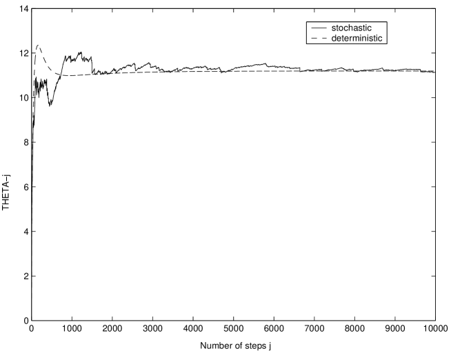
Figure 2: Comparison of the stochastic simulation and the deterministic computation

As a further validation, we ran the stochastic simulation for 10,000 steps, repeated 100 times, with parameters $p=0.3$ and $q=0.975$ as above, and compared it with a deterministic computation of the process using (8), (9) and (10) to calculate $E(F_{i}(k))$, the expected number of balls in each urn, instead of $F_{i}(k)$, the actual number of balls. The expected values will not in general be integral. The plots of the average $\Theta_{j}$ against $j$ for the stochastic simulation (solid line) and the deterministic computation (dashed line) are shown in Figure 2. The asymptotic average value of $\Theta_{j}$ for the deterministic computation was $11.192$ and for the stochastic simulation $11.145$.

4 A Model for Protein Networks

As mentioned in the introduction, exponential cutoff has been observed in several networks. Our model can be directly applied to web graphs [MBSA02], where balls represent web pages and pins represent links, to e-mail networks [EMB02], where balls represent e-mail accounts and pins represent e-mail messages, and to protein networks [JMBO01], where balls represent proteins and pins represent protein interactions. In a web graph removing a ball corresponds to deleting a web page, in an e-mail network removing a ball corresponds to a user’s e-mail account being removed from the network, and in a protein network removing a ball corresponds to gene loss resulting in the loss of a protein. The other category of network exhibiting exponential cutoff mentioned in the introduction, such as collaboration and actor networks, will be the subject of a follow-up paper.

We note that some types of network, viz. protein, collaboration and actor networks, are essentially undirected. Consequently, in our model, a new interaction between two proteins, for example, ought to be represented by two separate events, corresponding to the new interactions for each of the two proteins. This would correspond to taking in pairs the events of attaching a pin to a ball. We ignore this complication, but note that many of the models proposed, for example for the web graph, similarly ignore the difference between directed and undirected graphs (e.g. [BA99]).

As a proof of concept, we focus here on protein networks, and in particular we will examine a yeast protein interaction network [JMBO01]. This is an undirected graph that can be downloaded from www.nd.edu/~networks/database/protein. To obtain the values for $\varrho$ and $q$ we performed a nonlinear regression on a log-log transformation of the degree distribution of the yeast network data obtained from this website, fitting to the equation

$$y=a-(\varrho+1)x+\ln(q)\exp(x)$$ (25)

implied by (19), where $a$ is a constant. The values of $\varrho$ and $q$ obtained from the regression of the complete yeast data set are $\varrho=1.065$ and $q=0.9642$.

We next performed a stochastic simulation to test the validity of our model. In order to carry out the simulation we require values of $p$ and $k$. From (3) and (9) using the fact that $\varrho\approx(k\beta_{k})^{-1}$, we obtain

$$\frac{balls_{k}}{k}\approx p-(1-p)(1-q),$$ (26)

and

$$\frac{pins_{k}}{k}\approx\varrho(1-p),$$ (27)

where $balls_{k}$ and $pins_{k}$ stand for the expected numbers of balls and pins in the urns at stage $k$, respectively. (The right-hand sides of (26) and (27) are the limiting values of the left-hand sides as $k$ tends to infinity.)

From these we obtain an equation for the branching factor $bf$, viz.

$$bf=\frac{pins_{k}}{balls_{k}}\approx\frac{\varrho(1-p)}{p-(1-p)(1-q)},$$ (28)

and from (28) we can derive

$$p\approx\frac{\varrho+bf(1-q)}{\varrho+bf(2-q)}.$$ (29)

From the original yeast data, the values of $balls_{k}$ and $pins_{k}$ were $1870$ and $4480$, respectively, which give a branching factor $bf=2.3957$. Using the values of $\varrho$ and $q$ from the regression and this value of $bf$, from (29) we obtain a value of $p=0.3245$ to use in the simulation. Using this value of $p$, from (26) or (27) we obtain a value of $k=6227$. (Alternatively, we could have used (24) to estimate $p$, giving the value $0.3026$. We preferred the previous method, as this avoids the sensitivity of the hypergeometric function for values of $q$ near $1$.)

We carried out 10 simulation runs of the stochastic process using these values of $p$, $q$ and $k$. Using the value of $pins_{k}$ from the simulations we obtained an estimate of $\varrho$ from (27). The average value for $balls_{k}$ was $1869$, for $pins_{k}$ was $4795$, and for $\varrho$ was $1.14$.

Although these values seem to provide a good fit to the original data, as a further validation we investigated the value of $\theta$. Its value can estimated from (6) as

$$\theta\approx\frac{sqpins_{k}}{pins_{k}},$$ (30)

where $sqpins_{k}$ is given by

$$sqpins_{k}=\sum_{i=1}^{k}i^{2}F_{i}(k).$$

The value $sqpins_{k}$ from the original data is $29140$. Using (30) this gives the empirical value $\theta=6.5045$.

We have three equations for $\theta$: the first is the approximation given by (30), the second is (23), and the third, derived from (13), is

$$\theta=\frac{1-\varrho(1-p)}{(1-p)(1-q)}-1,$$ (31)

remembering that $\varrho=1/\beta$.

Using the value $sqpins_{k}=40195$ from the simulation, the first estimate of $\theta$, from (30), is $8.3823$. The second estimate, from (23), is $9.3057$, while the third estimate, from (31), is $10.0629$. It can be seen that the empirical value of $\theta$ is not consistent with these estimates from the mean-field equations.

We suggest that one reason for this inconsistency is due to problems in fitting power-law type distributions, due to difficulties with non-monotonic fluctuations in the tail. (Another reason maybe the sensitivity of the nonlinear regression to the cutoff parameter $q$.) In particular, the presence of gaps in the degree distribution is the main manifestation of this problem. There is a gap in the degree distribution at $i$ if there are no nodes of degree $i$ but there exists some node of degree $j$, where $j>i$. We discussed this problem more fully in the context of a pure power-law distribution in [FLL05], and concluded that a preferable approach is to ignore all data points from the first gap onwards. Evidence of the advantage of discarding data points in the tail of the distribution was also given in [GMY04], who suggest the more radical approach of using only the first five data points.

Following this approach we only use the first 15 data points in the degree distribution, since the first gap occurs at $i=16$. The values of $\varrho$ and $q$ obtained from the nonlinear regression fitting (25) to the truncated data set, are $\varrho=0.5586$ and $q=0.879$. The first 15 data points as well as the computed regression curve are shown in Figure 3. Using these values of $\varrho$ and $q$ together with the values of $balls_{k}$ and $pins_{k}$ from the original data, we computed $p=0.2615$ from (29) and $k=10860$ from (26) or (27).

We then repeated the 10 stochastic simulations using the new values of $p,q$ and $k$. The average estimate for $balls_{k}$ was $1858$, for $pins_{k}$ was $4463$, and for $\varrho$ using the values of $pins_{k}$ from the simulations and (27) was $0.5565$. The first estimate of $\theta$, using (30) and the value $sqpins_{k}=24666$ from the simulation, was $5.5263$. The second estimate was $5.5660$ from (23), while the third estimate was $5.5743$ from (31). It can be seen that these estimates are significantly more consistent with the empirical values of $sqpins_{k}$ and $\theta$ from the original data set.

We then carried out a further verification of the applicability of our methodology. We computed the average number of balls in each urn over the second 10 simulation runs; the first urn that contained no balls in any of the simulations was urn 32. Next, we performed a nonlinear regression on the first 31 urn averages using (25), as before. The values of $\varrho$ and $q$ obtained from this regression were $\varrho=0.5624$ and $q=0.8880$, which are very close to the corresponding values obtained from the regression on the truncated data set.

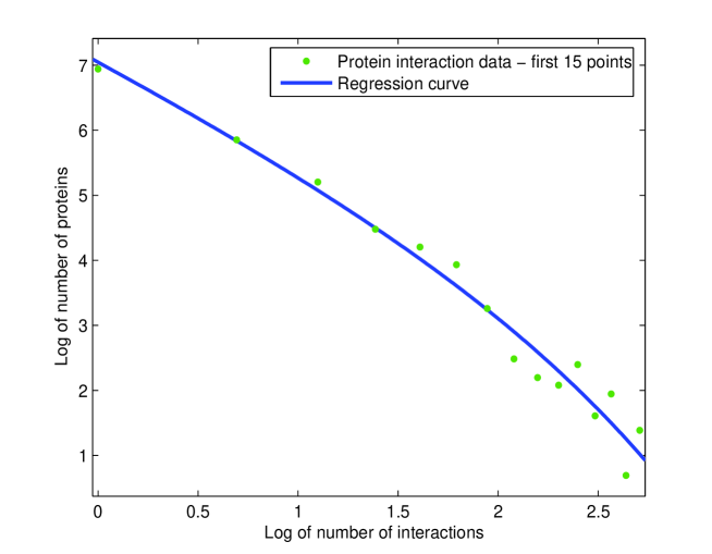
Figure 3: Yeast protein interaction network data

Jeong et al. [JMBO01] fit the data set to a power-law distribution with an exponential cutoff. However, they shift all the degree values by one, in order to obtain a better fit for small degrees. They report $q$ as approximately $\exp(-0.05)=0.9512$ and $\varrho$ as approximately $1.4$ (see supplementary information provided by the authors of [JMBO01]). In order to compare our results with theirs, we repeated the nonlinear regression on the first 15 data points, using (25), taking the degrees of the data points to be from 2 to 16. This gave the values $q=0.9828$ and $\varrho=1.513$, which are comparable to Jeong et al.’s results.

A confirmation of the existence of a cutoff can be obtained as follows. Let us assume there is no cutoff, i.e. $q=1$. Then, from (13) we have $\varrho=1/(1-p)$. Using this and (28) we derive $bf\approx\varrho/(\varrho-1)$, and thus $\varrho\approx bf/(bf-1)$. Now, since we are assuming there is no cutoff, we can perform a linear regression on the the log-log transformation of the first 15 data points, i.e. fitting to (25) with $q=1$, which yields $\varrho=1.251$.

Now, using the empirical branching factor $bf=2.3957$ from the original data, we can compute $\varrho$ as $2.3957/1.3957=1.7165$. This significantly deviates from the value $1.251$, obtained from the linear regression. Alternatively, we can compute the branching factor as $bf\approx 1.251/0.251=4.9841$, which deviates significantly from the empirical branching factor. These discrepancies lead us to conclude that a cutoff does exist, i.e. that $q<1$.

5 Concluding Remarks

We have presented an extension of Simon’s classical stochastic process, which results in a power-law distribution with an exponential cutoff, and for which the power-law exponent need not exceed two. When viewing this stochastic process in terms of an urn transfer model, the difference from the classical process is that, after a ball is chosen on the basis of preferential attachment, with probability $1-q$ the ball is discarded. Under our assumption that, for large $k$, the normalising factor $\beta_{k}$ can be approximated by the constant $\hat{\beta}_{k}$, we have derived the asymptotic formula (19), which shows that the distribution of the number of balls in the urns approximately follows a power-law distribution with an exponential cutoff. We note that we have, in fact, derived a more accurate formula (18) in terms of gamma functions.

Exponential cutoffs have been identified in protein, e-mail, actor and collaboration networks, and possibly in the web graph [MBSA02]; it is likely exponential cutoffs also occur in other complex networks. Our model assumes that balls are discarded rather than just becoming inactive as in actor and collaboration networks (the treatment of such networks with inactive nodes will be dealt in a subsequent paper). We have validated our model with data from a yeast protein network, showing that our model provides a possible explanation for the exponential cutoff. We have also presented convincing numerical evidence of the existence of a cutoff in this network.

In addition, we have checked that our model is consistent with the emergence of the power-law distribution for inlinks in the web graph. However, in this case $q$ is probably very close to one [MBSA02], and this may be the reason that we have not managed to establish the existence of an exponential cutoff for the web graph.

References

- [AB02] R. Albert and A.-L. Barabási. Statistical mechanics of complex networks. Reviews of Modern Physics, 74:47–97, 2002.
- [AH01] L.A. Adamic and B.A. Huberman. The Web’s hidden order. Communications of the ACM, 44(9):55–59, 2001.
- [AJB00] R. Albert, H. Jeong, and A.-L. Barabási. Error and attack tolerance of complex networks. Nature, 406:378–382, 2000.
- [ALPH01] L.A. Adamic, R.M. Lukose, A.R. Puniyani, and B.A. Huberman. Search in power-law networks. Physical Review E, 64:046135–1–046135–8, 2001.
- [AM01] M. Adler and M. Mitzenmacher. Towards compressing web graphs. In Proceedings of IEEE Data Compression Conference, pages 203–212, Snowbird, Utah, 2001.
- [AS72] M. Abramowitz and I.A. Stegun, editors. Handbook of Mathematical Functions with Formulas, Graphs and Mathematical Tables. Dover, New York, NY, 1972.
- [ASBS00] L.A.N. Amaral, A. Scala, M. Barthélémy, and H.E. Stanley. Classes of small-world networks. Proceedings of the National Academy of Sciences of the United States of America, 97:11149–11152, 2000.
- [BA99] A.-L. Barabási and R. Albert. Emergence of scaling in random networks. Science, 286:509–512, 1999.
- [BE01] S. Bornholdt and H. Ebel. World Wide Web scaling exponent from Simon’s 1955 model. Physical Review E, 64:035104–1–035104–4, 2001.
- [BKM+00] A. Broder, R. Kumar, F. Maghoul, P. Raghavan, A. Rajagopalan, R. Stata, A. Tomkins, and J. Wiener. Graph structure in the Web. Computer Networks, 33:309–320, 2000.
- [DM00] S.N. Dorogovtsev and J.F.F. Mendes. Evolution of networks with aging of sites. Physical Review E, 62:1842–1845, 2000.
- [EMB02] H. Ebel, L.-I. Mielsch, and S. Bornholdt. Scale-free topology of e-mail networks. Physical Review E, 66:035103–1–035103–4, 2002.
- [FLL05] T.I. Fenner, M. Levene, and G. Loizou. A stochastic model for the evolution of the web allowing link deletion. ACM Transactions on Internet Technology, August, 2005. To appear; also appears in the Condensed Matter Archive, cond-mat/0304316.
- [GMY04] M.L. Goldstein, S.A. Morris, and G.G. Yen. Problems with fitting to the power-law distribution. Condensed Matter Archive, cond-mat/0402322, 2004.
- [Gro02] J.W. Grossman. Patterns of collaboration in mathematical research. SIAM News, 35(9), November 2002.
- [JK77] N.L. Johnson and S. Kotz. Urn Models and their Application: An Approach to Modern Discrete Probability. Wiley Series in Probability and Mathematical Statistics. John Wiley & Sons, New York, NY, 1977.
- [JMBO01] H. Jeong, S.P. Mason, A.-L. Barabási, and Z.N. Oltvai. Lethality and centrality in protein networks. Nature, 411:41–42, 2001.
- [KRL00] P.L. Krapivsky, S. Redner, and F. Leyvraz. Connectivity of growing random networks. Physical Review Letters, 85:4629–4632, 2000.
- [KRR+00] R. Kumar, P. Raghavan, S. Rajagopalan, D. Sivakumar, A. Tomkins, and E. Upfal. Stochastic models for the web graph. In Proceedings of IEEE Symposium on Foundations of Computer Science, pages 57–65, Redondo Beach, Ca., 2000.
- [LFLW02] M. Levene, T.I. Fenner, G. Loizou, and R. Wheeldon. A stochastic model for the evolution of the Web. Computer Networks, 39:277–287, 2002.
- [MBSA02] S. Mossa, M. Barthélémy, H.E. Stanley, and L.A.N. Amaral. Truncation power law behavior in “scale-free” network models due to information filtering. Physical Review Letters, 88:138701–1–138701–4, 2002.
- [New01] M.E.J. Newman. The structure of scientific collaboration networks. Proceedings of the National Academy of Sciences of the United States of America, 98:404–409, 2001.
- [PFL+02] D.M. Pennock, G.W. Flake, S. Lawrence, E.J. Glover, and C.L. Giles. Winners don’t take all: Characterizing the competition for links on the web. Proceedings of the National Academy of Sciences of the United States of America, 99:5207–5211, 2002.
- [Red98] S. Redner. How popular is your paper? An empirical study of the citation distribution. European Physical Journal B, 4:131–134, 1998.
- [Ros83] S.M. Ross. Introduction to Stochastic Dynamic Programming. Academic Press, New York, NY, 1983.
- [Sim55] H.A. Simon. On a class of skew distribution functions. Biometrika, 42:425–440, 1955.
- [Sor00] D. Sornette. Critical Phenomema in the Natural Sciences: Chaos, Fractals, Selforganization and Disorder: Concepts and Tools. Springer Series in Synergetics. Springer-Verlag, Berlin, 2000.