Mixing patterns in networks

Abstract

We study assortative mixing in networks, the tendency for vertices in networks to be connected to other vertices that are like (or unlike) them in some way. We consider mixing according to discrete characteristics such as language or race in social networks and scalar characteristics such as age. As a special example of the latter we consider mixing according to vertex degree, i.e., according to the number of connections vertices have to other vertices: do gregarious people tend to associate with other gregarious people? We propose a number of measures of assortative mixing appropriate to the various mixing types, and apply them to a variety of real-world networks, showing that assortative mixing is a pervasive phenomenon found in many networks. We also propose several models of assortatively mixed networks, both analytic ones based on generating function methods, and numerical ones based on Monte Carlo graph generation techniques. We use these models to probe the properties of networks as their level of assortativity is varied. In the particular case of mixing by degree, we find strong variation with assortativity in the connectivity of the network and in the resilience of the network to the removal of vertices.

I Introduction

The techniques of statistical physics were developed to study the properties of systems of many interacting particles, atoms, or molecules, but their applicability is wider than this, and recent work has fruitfully applied these techniques to economies, ecosystems, social interactions, the Internet, and many other systems of current interest. The component parts of these systems, the analogs of atoms and molecules, such things as traders in a market, or computers on the Internet, are not usually connected together on a regular lattice as the atoms of a crystal are. Nor indeed do their patterns of connection normally fit any simple low-dimensional structure. Instead they fall on some more generalized “network,” which may be more or less random depending on the nature of the system. The broadening of the scope of statistical physics to cover these systems has therefore led us to the consideration of the structure and function of networks, as one of the fundamental steps to understanding real-world phenomena of many kinds. Useful reviews of work in this area can be found in Refs. Strogatz01, ; AB02, ; DM02, .

Recent studies of network structure have concentrated on a small number of properties that appear to be common to many networks and can be expected to affect the functioning of networked systems in a fundamental way. Among these, perhaps the best studied are the “small-world effect” TM69 ; WS98 , network transitivity or “clustering” WS98 , and degree distributions BA99b ; ASBS00 . Many other properties however have been examined and may be equally important, at least in some systems. Examples include resilience to the deletion of network nodes AJB00 ; Broder00 ; CEBH00 ; CNSW00 ; Holme02a , navigability or searchability of networks Kleinberg00proc ; ALPH01 ; WDN02 , community structure GN02 ; HHJ02 ; Guimera03 , and spectral properties Monasson99 ; GKK01 ; FDBV01 . In this paper we study another important network feature, the correlations between properties of adjacent network nodes known in the ecology and epidemiology literature as “assortative mixing.”

The very simplest representation of a network is a collection of points, usually called vertices or nodes, joined together in pairs by lines, usually called edges or links. More sophisticated network models may introduce other properties of the vertices or the edges. Edges for example may be directed—they point in one particular direction—or may have weights, lengths, or strengths. Vertices can also have weights or other numerical quantities associated with them, or may be drawn from some discrete set of vertex types. In the study of social networks, the patterns of connections between people in a society, it has long been known that edges do not connect vertices regardless of their property or type. Patterns of friendship between individuals for example are strongly affected by the language, race, and age of the individuals in question, among other things. If people prefer to associate with others who are like them, we say that the network shows assortative mixing or assortative matching. If they prefer to associate with those who are different it shows disassortative mixing. Friendship is usually found to be assortative by most characteristics.

Assortative mixing can have a profound effect on the structural properties of a network. For example, assortative mixing of a network by a discrete characteristic will tend to break the network up into separate communities. If people prefer to be friends with others who speak their own language, for example, then one might expect countries with more than one language to separate into communities by language. Assortative mixing by age could cause stratification of societies along age lines. And while the main focus of this paper is on social networks, it is reasonable to suppose that similar mixing effects are seen in non-social networks also. We will give some examples of this in Section III.1.

In this paper we study assortative mixing of various types using empirical network data, analytic models, and numerical simulation. We demonstrate that assortative (or disassortative) mixing is indeed present in many networks, show how it can be measured, and examine its effect on network structure and behavior. The outline of the paper is as follows. In Section II we study the effects of assortative mixing by discrete characteristics such as language or race. In Section III we study mixing by scalar properties such as age and particularly vertex degree; since degree is itself a property of the network topology, the latter type of mixing leads to some novel network structures not seen with other types. In Section IV we give our conclusions. A preliminary report of some of the results in this paper has appeared previously as Ref. Newman02f, .

II Discrete characteristics

In this section we consider assortative mixing according to discrete or enumerative vertex characteristics. Such mixing can be characterized by a quantity $e_{ij}$, which we define to be the fraction of edges in a network that connect a vertex of type $i$ to one of type $j$. On an undirected network this quantity is symmetric in its indices $e_{ij}=e_{ji}$, while on directed networks or bipartite networks it may be asymmetric. It satisfies the sum rules

$$\sum_{ij}e_{ij}=1,\qquad\sum_{j}e_{ij}=a_{i},\qquad\sum_{i}e_{ij}=b_{j},$$ (1)

where $a_{i}$ and $b_{i}$ are the fraction of each type of end of an edge that is attached to vertices of type $i$. On undirected graphs, where the ends of edges are all of the same type, $a_{i}=b_{i}$ .

For example, Table 1 shows data on the values of $e_{ij}$ for mixing by race among sexual partners in a 1992 study carried out in the city of San Francisco, California CCKF92 . This part of the study focused on heterosexuals, so this is a bipartite network, the two vertex types representing men and women, with edges running only between vertices of unlike types. This means that in this case the ends of an edge are different and the matrix $e_{ij}$ is asymmetric. As the table shows, mixing is highly assortative in this network, with individuals strongly preferring partners from the same group as themselves.

		women
		black	hispanic	white	other	$a_{i}$
men	black	0.258	0.016	0.035	0.013	0.323
	hispanic	0.012	0.157	0.058	0.019	0.247
	white	0.013	0.023	0.306	0.035	0.377
	other	0.005	0.007	0.024	0.016	0.053
$b_{i}$		0.289	0.204	0.423	0.084

Table 1: The mixing matrix $e_{ij}$ and the values of $a_{i}$ and $b_{i}$ for sexual partnerships in the study of Catania et al. CCKF92 . After Morris Morris95 .

II.1 Measuring discrete assortative mixing

To quantify the level of assortative mixing in a network we define an assortativity coefficient thus:

$$r={\sum_{i}e_{ii}-\sum_{i}a_{i}b_{i}\over 1-\sum_{i}a_{i}b_{i}}={\mathop{\rm Tr}\mathbf{e}-\|\,\mathbf{e}^{2}\,\|\over 1-\|\,\mathbf{e}^{2}\,\|},$$ (2)

where $\mathbf{e}$ is the matrix whose elements are $e_{ij}$ and $\|\,\mathbf{x}\,\|$ means the sum of all elements of the matrix $\mathbf{x}$. This formula gives $r=0$ when there is no assortative mixing, since $e_{ij}=a_{i}b_{j}$ in that case, and $r=1$ when there is perfect assortative mixing and $\sum_{i}e_{ii}=1$. If the network is perfectly disassortative, i.e., every edge connects two vertices of different types, then $r$ is negative and has the value

$$r_{\rm min}=-{\sum_{i}a_{i}b_{i}\over 1-\sum_{i}a_{i}b_{i}},$$ (3)

which lies in general in the range $-1\leq r<0$. One might ask what this value signifies. Why do we not simply have $r=-1$ for a perfectly disassortative network? The answer is that a perfectly disassortative network is normally closer to a randomly mixed network than is a perfectly assortative network. When there are several different vertex types (e.g., four in the case shown in Table 1) then random mixing will most often pair unlike vertices, so that the network appears to be mostly disassortative. Therefore it is appropriate that the value $r=0$ for the random network should be closer to that for the perfectly disassortative network than for the perfectly assortative one.

A quantity with properties similar to those of Eq. (2) has been proposed previously by Gupta et al. GAM89 . However the definition of Gupta et al. gives misleading results in certain situations, such as, for example, when one type of vertex is much less numerous than other types, as is the case in Table 1. In this paper therefore we use Eq. (2), which doesn’t suffer from this problem. The difference between the two measures is discussed in more detail in Appendix A.

Using the values from Table 1 in Eq. (2), we find that $r=0.621$ for the network of sexual partnerships, implying, as we observed already, that this network is strongly assortative by race—individuals draw their partners from their own group far more often than one would expect on the basis of pure chance.

As another example of the application of Eq. (2), consider the network studied by Girvan and Newman GN02 representing the timetable of American college football games, in which vertices represent universities and colleges, and edges represent regular season games between teams during the year in question. Colleges are grouped into “conferences,” which are defined primarily by geography, and teams normally play more often against other teams in their own conference than they do against teams from other conferences. In other words, there should be assortative mixing of colleges by conference in the schedule network. For the 2000 season schedule studied in Ref. GN02, , we find a value for the assortativity coefficient of $r=0.586$, again indicating strong assortative mixing, i.e., colleges do indeed play games with their conference partners to a substantially greater degree than one would expect in a randomly mixed network.

It is also useful to know the expected statistical error on the value of $r$, so that we can evaluate the significance of our results. One way to calculate this error is to use the jackknife method Efron79 . Regarding each of the $M$ edges in a network as an independent measurement of the contributions to the elements of the matrix $\mathbf{e}$, we can show that the expected standard deviation $\sigma_{r}$ on the value of $r$ satisfies

$$\sigma_{r}^{2}=\sum_{i=1}^{M}(r_{i}-r)^{2},$$ (4)

where $r_{i}$ is the value of $r$ for the network in which the $i$th edge is removed. For example, in the case of the matrix of Table 1 this gives $\sigma_{r}=0.014$, which, when compared with the value $r=0.621$ shows that our finding of assortative mixing is strongly statistically significant—a $40\sigma$ result.

Although it has a rather different physical interpretation, the coefficient $r$ is mathematically similar to the intraclass correlation coefficients used in statistics to compare measurements across different groups in a population Fleiss81 . Standard results for errors on intraclass correlations can be adapted to the present case to show that another estimate of the error on $r$ is FCE69

$$\sigma_{r}^{2}={1\over M}\,{\sum_{i}a_{i}b_{i}+\bigl{[}\sum_{i}a_{i}b_{i}\bigr{]}^{2}-\sum_{i}a_{i}^{2}b_{i}-\sum_{i}a_{i}b_{i}^{2}\over 1-\sum_{i}a_{i}b_{i}},$$ (5)

which gives $\sigma_{r}=0.012$ for the data of Table 1, comparable with the jackknife method. Either method for estimating $\sigma_{r}$ will be adequate for most purposes—the choice between them is a matter of convenience.

II.2 Models of discrete assortative networks

The generalized random graph models of networks studied in the past by various authors BC78 ; Luczak92 ; MR95 ; MR98 ; ACL00 ; NSW01 ; NWS02 can be extended to the case of assortative mixing on discrete characteristics. Suppose we are told the degree distribution $p_{k}^{(i)}$ for vertices of type $i=1\ldots n$ in a network and the value of the mixing matrix $e_{ij}$. Implicitly, we are also told the values of the quantities $a_{i}$ and $b_{i}$, since we can extract them from $e_{ij}$ using Eq. (1). We consider the ensemble of all graphs with these values of $p_{k}^{(i)}$ and $e_{ij}$, which gives us a random graph model similar in spirit to that of Refs. BC78, ; Luczak92, ; MR95, ; MR98, ; ACL00, ; NSW01, ; NWS02, for the case of specified degree distribution only. Many properties of this ensemble can be calculated exactly in the limit of large system size, as we now demonstrate.

Suppose that a vertex of type $i$ has degree $k$. The $k$ vertices at the other ends of the edges attached to this vertex are divided among the $n$ possible vertex types according to some partition $\{r_{1},r_{2},\ldots r_{n}\}$, where $\sum_{j}r_{j}=k$. The probability that the partition $\{r_{j}\}$ takes a particular value is given by the multinomial distribution

$$P^{(i)}(k,\{r_{j}\})=k!\prod_{j}{1\over r_{j}!}\biggl{[}{e_{ij}\over\sum_{j}e_{ij}}\biggr{]}^{r_{j}}.$$ (6)

Now, generalizing Ref. NSW01, , we define a generating function for the distributions of the numbers of edges connecting to each type of vertex:

$$G_{0}^{(i)}(x_{1},x_{2},\ldots x_{n}) =$$ (7)

$$\sum_{k=0}^{\infty}p_{k}^{(i)}\sum_{\{r_{j}\}}\delta\bigl{(}k,\sum_{j}r_{j}\bigr{)}P^{(i)}\bigl{(}k,\{r_{j}\}\bigr{)}x_{1}^{r_{1}}x_{2}^{r_{2}}\ldots x_{n}^{r_{n}}.$$

Performing the sum over $\{r_{j}\}$, this gives

$$G_{0}^{(i)}(x_{1},x_{2},\ldots x_{n}) = \sum_{k}p_{k}^{(i)}\Biggl{[}{\sum_{j}e_{ij}x_{j}\over\sum_{j}e_{ij}}\Biggr{]}^{k}$$ (8)

$$= G_{0}^{(i)}\Biggl{(}{\sum_{j}e_{ij}x_{j}\over\sum_{j}e_{ij}}\Biggr{)},$$

where

$$G_{0}^{(i)}(x)=\sum_{k}p_{k}^{(i)}x^{k}$$ (9)

is the fundamental generating function for the degree distribution $p_{k}^{(i)}$, as defined in Ref. NSW01, . Similarly, for the edges connected to a vertex of type $i$ reached by following a randomly chosen edge on the graph we have

$$G_{1}^{(i)}(x_{1},x_{2},\ldots x_{n})=G_{1}^{(i)}\Biggl{(}{\sum_{j}e_{ij}x_{j}\over\sum_{j}e_{ij}}\Biggr{)},$$ (10)

with

$$G_{1}^{(i)}(x)={\sum_{k}kp_{k}^{(i)}x^{k-1}\over\sum_{k}kp_{k}^{(i)}}={1\over z_{i}}{{\rm d}G_{0}^{(i)}\over{\rm d}x}\biggr{|}_{x=1},$$ (11)

where $z_{i}\equiv{G_{0}^{(i)}}^{\prime}(1)$ is the mean degree for type $i$ vertices.

Now we consider the total number of vertices reachable by following an edge that arrives at a vertex of type $i$. This number has a distribution that is generated by a generating function $H_{1}^{(i)}$ satisfying a self-consistency condition of the form

$$H_{1}^{(i)}(x)=xG_{1}^{(i)}(H_{1}^{(1)}(x),\ldots H_{1}^{(n)}(x)).$$ (12)

And similarly the distribution of the number of vertices reachable from a randomly chosen vertex of type $i$ is generated by

$$H_{0}^{(i)}(x)=xG_{0}^{(i)}(H_{1}^{(1)}(x),\ldots H_{1}^{(n)}(x)).$$ (13)

By solving these two equations simultaneously, we can derive the complete component size distribution in our model. Here however, we will just calculate some of the more important average statistics of our networks from the generating functions. For example, the mean number $s_{i}$ of vertices reachable from a vertex of type $i$ is

$$s_{i}={{\rm d}H_{0}^{(i)}\over\!{\rm d}x}\biggr{|}_{x=1}=1+{G_{0}^{(i)}}^{\prime}(1){\sum_{j}e_{ij}{H_{1}^{(j)}}^{\prime}(1)\over\sum_{j}e_{ij}}.$$ (14)

We can write this in matrix form thus:

$$\mathbf{s}=\mathbf{1}+\mathbf{m}_{0}\cdot\mathbf{H}_{1}^{\prime}(1),$$ (15)

where $\mathbf{m}_{0}$ is the matrix with elements $z_{i}{e_{ij}/a_{i}}$. Differentiating Eq. (12), we then find that

$$\mathbf{s}=\mathbf{1}+\mathbf{m}_{0}\cdot[\mathbf{I}-\mathbf{m}_{1}]^{-1}\cdot\mathbf{1},$$ (16)

where $\mathbf{1}$ is the vector whose elements are all 1, and the matrix $\mathbf{m}_{1}$ has elements

$$[\mathbf{m}_{1}]_{ij}={z_{2}^{(i)}\over z_{1}^{(i)}}{e_{ij}\over a_{i}},$$ (17)

with $z_{1}^{(i)}\equiv z_{i}$ being the mean degree of type $i$ vertices and $z_{2}^{(i)}$ being the mean number of neighbors at distance two from a type $i$ vertex.

When the density of edges on the graph is small, $\mathbf{s}$ in Eq. (16) is finite, but it grows with increasing density and then diverges when the determinant of the matrix $\mathbf{I}-\mathbf{m}_{1}$ reaches its first zero. This point marks the phase transition at which a giant component first appears in the network, similar to the phase transition seen in uncorrelated random graphs. The condition $\det(\mathbf{I}-\mathbf{m}_{1})=0$ for the position of the phase transition is the equivalent of the condition of Molloy and Reed MR95 for the position of the phase transition in an uncorrelated random graph of arbitrary degree distribution.

The size of the giant component can also be calculated in a straightforward manner. We define $u_{i}$ to be the probability that a vertex of type $i$, reached by following a randomly chosen edge in the graph, does not belong to the giant component. This probability is precisely equal to the probability that none of the neighbors of that vertex are themselves members of the giant component, and hence $u_{i}$ satisfies the self-consistency condition

$$u_{i}=G_{1}^{(i)}(u_{1},\ldots u_{n}).$$ (18)

The probability that a randomly chosen vertex of type $i$ is not a member of the giant component is then $G_{0}^{(i)}(u_{1},\ldots u_{n})$, and the overall fraction $S$ of vertices that are in the giant component is given by

$$S=1-\sum_{i}{a_{i}\over z_{i}}G_{0}^{(i)}(u_{1},\ldots u_{n}),$$ (19)

where we have made use of the fact that the fraction of vertices of type $i$ in the network is equal to $a_{i}/z_{i}$.

The simultaneous solution of Eqs. (18) and (19) gives us the value of $S$ for our network. In many cases we find that these equations are not solvable in closed form, but they can easily be solved numerically by iteration of Eq. (18) from suitable starting values for the $u_{i}$, and then substituting the result into (19).

II.3 Simulating discrete assortative networks

We would also like to be able to generate random networks with a given level of assortative mixing, in order to check our analytical results and also for use as substrates for other models, such as, for example, epidemiological models. A simple algorithm for achieving this is the following.

1. We first choose a size for our graph in terms of the number $M$ of edges and we draw $M$ edges from the distribution $e_{ij}$. That is, we generate $M$ edges, each one identified by the types of the vertices that it connects, in some manner such that the fraction of edges connecting vertices of types $i$ and $j$ tends to $e_{ij}$ as $M$ becomes large. In practice, a simple transformation method works well NB99 .

2. We count the number of ends of edges of each type $i$, to give the sums $m_{i}$ of the degrees of vertices in each class. We calculate the expected number $n_{i}$ of vertices of each type from $n_{i}=m_{i}/z_{i}$ (rounded to the nearest integer), where $z_{i}$ is the desired mean degree of vertices of type $i$.

3. We draw $n_{i}$ vertices from the desired degree distribution $p_{k}^{(i)}$ for type $i$. In general the degrees of these vertices will not sum exactly to $m_{i}$ as we want them to. So we choose one vertex at random, discard it, and draw another from the distribution $p_{k}^{(i)}$ until the sum does equal $m_{i}$.

4. We pair up the $m_{i}$ ends of edges of type $i$ at random with the vertices we have generated, so that each vertex has the number of attached edges corresponding to its chosen degree.

5. We repeat from step 3 for each vertex type.

This method correctly generates assortatively mixed graphs with the given $e_{ij}$ in the limit of large graph size. In Section III.3 of this paper we give some examples of simulations of assortatively mixed networks.

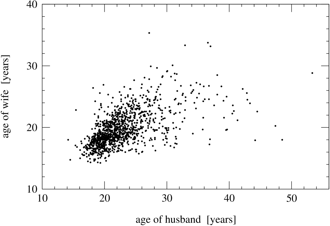
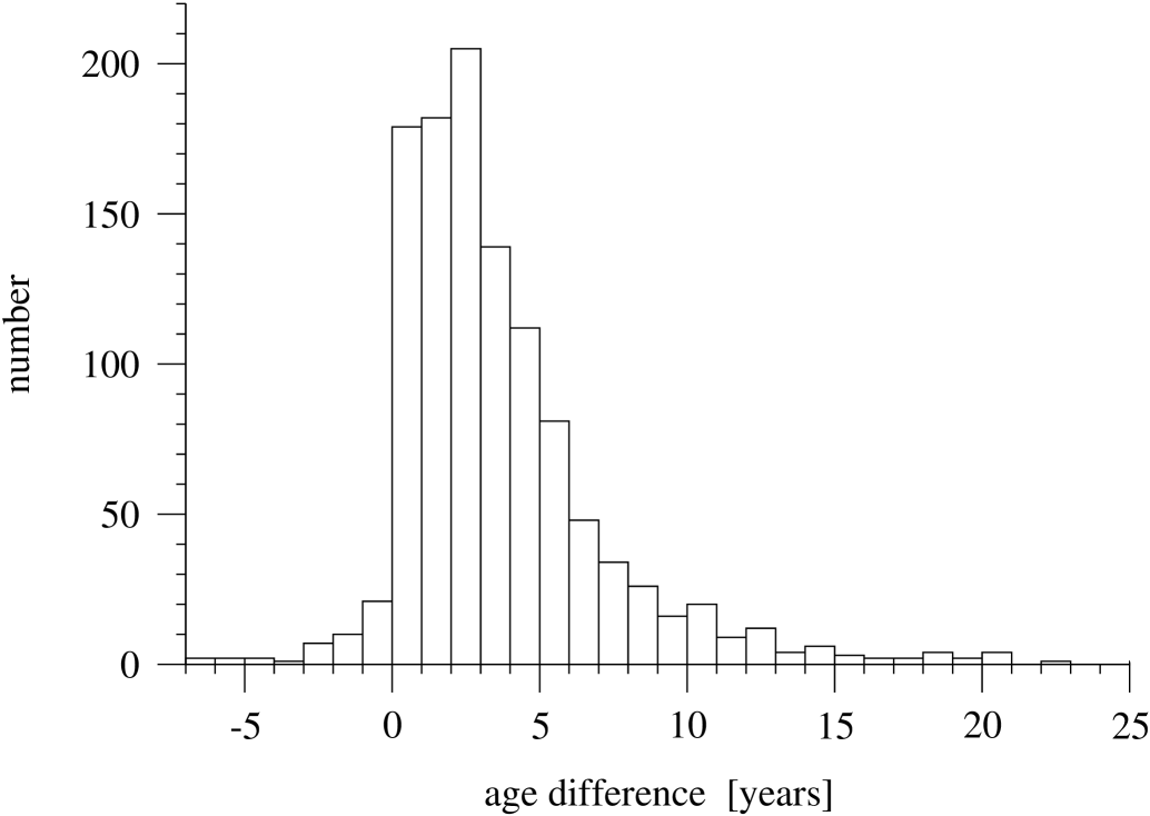
Figure 1: Top: scatter plot of the ages of 1141 married couples at time of marriage, from the 1995 US National Survey of Family Growth NSFG97 . Bottom: a histogram of the age differences (male minus female) for the same data.

III Assortative mixing by scalar properties

A similar, but distinct, form of assortative mixing is mixing that depends on one or more scalar properties of network vertices. A classic example of mixing of this type seen in many social networks is assortative mixing by age. In Fig. 1 (top panel) we show a scatter plot of the ages of marriage partners in the 1995 US National Survey of Family Growth NSFG97 . As is clear from the figure, there is a strong positive correlation between the ages, with most of the density in the distribution lying along a rough diagonal in the plot; people, it appears, prefer to marry others of about the same age, although there is some bias towards husbands being older than their wives. In the bottom panel of the same figure we show a histogram of the age differences in the study, which emphasizes the same conclusion .

By analogy with the developments of Section II, we can define a quantity $e_{xy}$, which is the fraction of all edges in the network that join together vertices with values $x$ and $y$ for the age or other scalar variable of interest. The values $x$ and $y$ might be either discrete in nature (e.g., integers, such as age to the nearest year) or continuous (exact age), making $e_{xy}$ either a matrix or a function of two continuous variables. Here, for simplicity, we concentrate on the discrete case, but generalization to the continuous case is straightforward.

As before, we can use the matrix $e_{xy}$ to define a measure of assortativity. We first note that $e_{xy}$ satisfies the sum rules

$$\sum_{xy}e_{xy}=1,\qquad\sum_{y}e_{xy}=a_{x},\qquad\sum_{x}e_{xy}=b_{y},$$ (20)

where $a_{x}$ and $b_{y}$ are, respectively, the fraction of edges that start and end at vertices with values $x$ and $y$. (On an undirected, unipartite graph, $a_{x}=b_{x}$.) Then, if there is no assortative mixing $e_{xy}=a_{x}b_{y}$. If there is assortative mixing one can measure it by calculating the standard Pearson correlation coefficient thus:

$$r={\sum_{xy}xy(e_{xy}-a_{x}b_{y})\over\sigma_{a}\sigma_{b}},$$ (21)

where $\sigma_{a}$ and $\sigma_{b}$ are the standard deviations of the distributions $a_{x}$ and $b_{y}$. The value of $r$ lies in the range $-1\leq r\leq 1$, with $r=1$ indicating perfect assortativity and $r=-1$ indicating perfect disassortativity (i.e., perfect negative correlation between $x$ and $y$). For the age data from Fig. 1, for example, we find that $r=0.574$, indicating strong assortative mixing once more.

One can construct in a straightforward manner a random graph model of a network with this type of mixing exactly analogous to the model presented in Section II.2. It is also possible to generate random representative networks from the ensemble defined by $e_{xy}$ using the algorithm described in Section II.3. In this paper however, rather than working further on the general type of mixing described here, we will concentrate on one special example of assortative mixing by a scalar property which is particularly important for many of the networks we are interested in, namely mixing by vertex degree.

III.1 Mixing by vertex degree

In general, scalar assortative mixing of the type described above requires that the vertices of the network of interest have suitable scalar properties attached to them, such as age or income in social networks. In many cases, however, data are not available for these properties to allow us to assess whether the network is assortatively mixed. But there is one scalar vertex property that is always available for every network, and that is vertex degree. So long as we know the network structure we always know the degree of a vertex, and then we can ask whether vertices of high degree preferentially associate with other vertices of high degree. Do the gregarious people hang out with other gregarious people? This has been a topic of considerable discussion in the physics literature PVV01 ; MS02b ; DMS02 ; VW02 ; BPV02 . As we will show, many real-world networks do show significant assortative (or disassortative) mixing by vertex degree.

Assortative mixing by degree can be quantified in exactly the same way as for other scalar properties of vertices, using Eq. (21). Taking the example of an undirected network and using the notation of Ref. Newman02f, , we define $e_{jk}$ to be the fraction of edges that connect vertices of degrees $j$ and $k$. In fact, we choose $j$ and $k$ to be the excess degrees of the vertices (also called remaining degree in Ref. Newman02f, ), which are one less than the degrees of the vertices themselves. This is because in most cases we are interested in the number of edges attached to a vertex other than the particular edge we are looking at at the moment.

If the degree distribution of the graph as a whole is $p_{k}$, i.e., $p_{k}$ is the probability that a randomly chosen vertex will have degree $k$, then the excess degree of the vertex at the end of an edge is distributed according to NSW01

$$q_{k}={(k+1)p_{k+1}\over z},$$ (22)

where $z=\sum_{k}kp_{k}$ is the mean degree in the network. The distribution $q_{k}$ is related to $e_{jk}$ via

$$\sum_{j}e_{jk}=q_{k}.$$ (23)

The correct assortativity coefficient for mixing by vertex degree in an undirected network is

$$r={\sum_{jk}jk(e_{jk}-q_{j}q_{k})\over\sigma_{q}^{2}},$$ (24)

where $\sigma_{q}$ is the standard deviation of the distribution $q_{k}$. For a directed network the equivalent expression is

$$r={\sum_{jk}jk(e_{jk}-q^{\rm in}_{j}q^{\rm out}_{k})\over\sigma_{\rm in}\sigma_{\rm out}},$$ (25)

where $e_{jk}$ is now the probability that a randomly chosen directed edge leads into a vertex of in-degree $j$ and out of a vertex of out-degree $k$ . For the purposes of calculating $r$ for an actual network of specified vertices and edges, we can rewrite this in the form

$$r={\sum_{i}j_{i}k_{i}-M^{-1}\sum_{i}j_{i}\sum_{i^{\prime}}k_{i^{\prime}}\over\sqrt{\Bigl{[}\sum_{i}j_{i}^{2}-M^{-1}\bigl{(}\sum_{i}j_{i}\bigr{)}^{2}\Bigr{]}\Bigl{[}\sum_{i}k_{i}^{2}-M^{-1}\bigl{(}\sum_{i}k_{i}\bigr{)}^{2}\Bigr{]}}},$$ (26)

where $j_{i}$ and $k_{i}$ are the excess in-degree and out-degree of the vertices that the $i$th edge leads into and out of respectively, and $M$ is again the number of edges. For an undirected network we can use the same formula—we simply replace each undirected edge by two directed ones leading in opposite directions. Alternatively, one can apply directly the formula given in Ref. Newman02f, , Eq. (4), to the undirected network. As before, errors on the measured values of $r$ can be calculated using the jackknife method and Eq. (4).

         network type size $n$ assortativity $r$ error $\sigma_{r}$ ref. $\mbox{social}\left\{\rule{0.0pt}{37.0pt}\right.$ physics coauthorship undirected $52\,909$ $\phantom{-}0.363$ $0.002$ a biology coauthorship undirected $1\,520\,251$ $\phantom{-}0.127$ $0.0004$ a mathematics coauthorship undirected $253\,339$ $\phantom{-}0.120$ $0.002$ b film actor collaborations undirected $449\,913$ $\phantom{-}0.208$ $0.0002$ c company directors undirected $7\,673$ $\phantom{-}0.276$ $0.004$ d student relationships undirected $573$ $-0.029$ $0.037$ e email address books directed $16\,881$ $\phantom{-}0.092$ $0.004$ f $\mbox{technological}\left\{\rule{0.0pt}{22.0pt}\right.$ power grid undirected $4\,941$ $-0.003$ $0.013$ g Internet undirected $10\,697$ $-0.189$ $0.002$ h World-Wide Web directed $269\,504$ $-0.067$ $0.0002$ i software dependencies directed $3\,162$ $-0.016$ $0.020$ j $\mbox{biological}\left\{\rule{0.0pt}{26.0pt}\right.$ protein interactions undirected $2\,115$ $-0.156$ $0.010$ k metabolic network undirected $765$ $-0.240$ $0.007$ l neural network directed $307$ $-0.226$ $0.016$ m marine food web directed $134$ $-0.263$ $0.037$ n freshwater food web directed $92$ $-0.326$ $0.031$ o

Table 2: Size $n$, degree assortativity coefficient $r$, and expected error $\sigma_{r}$ on the assortativity, for a number of social, technological, and biological networks, both directed and undirected. Social networks: coauthorship networks of (a) physicists and biologists Newman01a and (b) mathematicians GI95 , in which authors are connected if they have coauthored one or more articles in learned journals; (c) collaborations of film actors in which actors are connected if they have appeared together in one or more movies WS98 ; ASBS00 ; (d) directors of Fortune 1000 companies for 1999, in which two directors are connected if they sit on the board of directors of the same company DYB01 ; (e) romantic (not necessarily sexual) relationships between students at a US high school BMS02 ; (f) network of email address books of computer users on a large computer system, in which an edge from user A to user B indicates that B appears in A’s address book NFB02 . Technological networks: (g) network of high voltage transmission lines in the Western States Power Grid of the United States WS98 ; (h) network of direct peering relationships between autonomous systems on the Internet, April 2001 Chen02 ; (i) network of hyperlinks between pages in the World-Wide Web domain nd.edu, circa 1999 AJB99 ; (j) network of dependencies between software packages in the GNU/Linux operating system, in which an edge from package A to package B indicates that A relies on components of B for its operation. Biological networks: (k) protein–protein interaction network in the yeast S. Cerevisiae Jeong01 ; (l) metabolic network of the bacterium E. Coli Jeong00 ; (m) neural network of the nematode worm C. Elegans WSTB86 ; WS98 ; tropic interactions between species in the food webs of (n) Ythan Estuary, Scotland HBR96 and (o) Little Rock Lake, Wisconsin Martinez91 .

In Table 2 we show the measured values of $r$ for degree correlations in undirected and directed networks of a variety of different types, along with the expected errors on these values. The table reveals an interesting feature: essentially all the social networks examined are significantly assortative by degree, i.e., high degree vertices tend to be connected to other high degree vertices, while all the technological and biological networks are disassortative. Three of the values for $r$, for the network of student relationships, the power grid, and the graph of software dependencies, are null results, meaning that they are not statistically different from zero. All the others however fit the pattern clearly, with positive values of $r$ for the social networks and negative values for all the others.

What is the explanation of this phenomenon? In all probability, there are a number of different mechanisms at work. Some possibilities are the following:

1. In the social networks it is entirely possible, and is often assumed in the sociological literature, that similar people do attract one another, and therefore that there could be a real preference among gregarious people for association with other gregarious people, and similarly for hermits.

2. On the other hand, the networks of collaborations between academics, actors, and businesspeople considered here are affiliation networks, i.e., networks in which people are connected together by membership of common groups (authors of a paper, actors in a film, etc.). Since all members of a group are thus connected to all other members, the positive correlations between degrees may at least in part reflect the fact that the members of a large (small) group are connected to the other members of the same large (small) group.

3. In the Internet and the World-Wide Web there may be organizational reasons for degree anti-correlation between vertices. The high-degree vertices in these networks are often connectivity providers (Internet) or directories (Web), which by definition tend to be connected to the “little people”—the individual service subscribers in the case of the Internet or the individual web-pages on the Web.

4. Maslov and Sneppen MS02b have shown that disassortativity can be produced as a finite-size effect by the constraint that no two vertices in a network are connected by more than one edge. This constraint causes high-degree vertices to “repel” one another, producing negative values of $r$. This explanation could account for at least a part of the disassortative mixing we see in the Internet, the protein and metabolic networks, and the food webs, although it cannot be applied directly to the Web and neural networks, for which vertex pairs can and often do have more than one connection.

It appears therefore that some of the degree correlations we see in our networks could have real social or organizational origins, while others may be artifacts of the types of networks we are looking at and the constraints that are placed on their structure.

III.2 Models of assortative mixing by degree

In Ref. Newman02f, we studied the ensemble of graphs that have a specified value of the matrix $e_{jk}$ and solved exactly for its average properties using generating function methods similar to those of Section II.2. We showed that the phase transition at which a giant component first appears in such networks occurs at a point given by $\det(\mathbf{I}-\mathbf{m})=0$, where $\mathbf{m}$ is the matrix with elements $m_{jk}=ke_{jk}/q_{j}$. One can also calculate exactly the size of the giant component, and the distribution of sizes of the small components below the phase transition. While these developments are mathematically elegant, however, their usefulness is limited by the fact that the generating functions involved are rarely calculable in closed form for arbitrary specified $e_{jk}$, and the determinant of the matrix $\mathbf{I}-\mathbf{m}$ almost never is. In this paper, therefore, we take an alternative approach, making use of computer simulation.

We would like to generate on a computer a random network having, for instance, a particular value of the matrix $e_{jk}$. (This also fixes the degree distribution, via Eq. (23).) In Ref. Newman02f, we discussed one possible way of doing this using an algorithm similar that of Section II.3. One would draw edges from the desired distribution $e_{jk}$ and then join the degree $k$ ends randomly in groups of $k$ to create the network. (This algorithm has also been discussed recently by Dorogovtsev et al. DMS02 .) As we pointed out, however, this algorithm is flawed because in order to create a network without any dangling edges the number of degree $k$ ends must be a multiple of $k$ for all $k$. It is very unlikely that these constraints will be satisfied by chance, and there does not appear to be any simple way of arranging for them to be satisfied without introducing bias into the ensemble of graphs. Instead, therefore, we use a Monte Carlo sampling scheme which is essentially equivalent to the Metropolis–Hastings method widely used in the mathematical and social sciences for generating model networks Strauss86 ; Snijders02 . The algorithm is as follows.

1. Given the desired edge distribution $e_{jk}$, we first calculate the corresponding distribution of excess degrees $q_{k}$ from Eq. (23), and then invert Eq. (22) to find the degree distribution:

   $$p_{k}={q_{k-1}/k\over\sum_{j}q_{j-1}/j}.$$ (27)

   Note that this equation cannot tell us how many vertices there are of degree zero in the network. This information is not contained in the edge distribution $e_{jk}$ since no edges connect to degree-zero vertices, and so must be specified separately. On the other hand, most of the properties of networks with which we will be concerned here don’t depend on the number of degree-zero vertices, so we can safely set $p_{0}=0$ for the purposes of this paper.

2. We draw a degree sequence, a specific set $k_{i}$ of degrees of the vertices $i=1\ldots N$, from the distribution $p_{k}$, and connect vertices together randomly in pairs to generate a random graph, as described, for instance, by Molloy and Reed MR95 .

3. We choose two edges at random from the graph. Let us denote these by the vertex pairs $(v_{1},w_{1})$ and $(v_{2},w_{2})$ that they connect.

4. We measure the excess degrees $j_{1},k_{1},j_{2},k_{2}$ of the vertices $v_{1},w_{1},v_{2},w_{2}$ and then we remove the two edges and replace them with two new ones $(v_{1},v_{2})$ and $(w_{1},w_{2})$ with probability

   $$P=\Biggl{\{}\begin{array}[]{ll}\phantom{\bigg{|}}{\displaystyle e_{j_{1}j_{2}}e_{k_{1}k_{2}}\over\displaystyle e_{j_{1}k_{1}}e_{j_{2}k_{2}}}&\qquad\mbox{if $e_{j_{1}j_{2}}e_{k_{1}k_{2}}<e_{j_{1}k_{1}}e_{j_{2}k_{2}}$}\\ \phantom{\big{|}}1&\qquad\mbox{otherwise.}\end{array}$$ (28)

5. Repeat from step 3.

Clearly this swap procedure preserves the degree sequence. It is also ergodic over the set of graphs with that degree sequence, i.e., it can reach any graph within that set in a finite number of moves. To see this, consider any configuration of the graph other than the desired target configuration and choose any vertex pair that is not joined by an edge in that configuration but is joined by an edge in the target. These vertices must necessarily each be attached to at least one other edge that does not exist in the target configuration. Take these edges and perform the swap procedure on them. This always increases the number of edges that the configuration has in common with the target. And since it is always possible to do this, it immediately follows that any target configuration can be reached in at most $M$ such moves, where $M$ is the number of edges in the network. (Actually, $M-1$ will suffice, since the last edge will always automatically be in the correct position by a process of elimination.)

Our algorithm also satisfies detailed balance. We would like to sample graph configurations $\mu$ with probabilities 

$$p_{\mu}=\prod_{i=1}^{M}e_{j_{i}k_{i}},$$ (29)

where $j_{i},k_{i}$ are the excess degrees of the vertices at the ends of the $i$th edge. It is trivial to show that with the choice of transition probabilities given in Eq. (28), we satisfy detailed balance in the form

$$p_{\mu}P(\mu\to\nu)=p_{\nu}P(\nu\to\mu),$$ (30)

for all pairs $\mu,\nu$ of states.

Since our algorithm satisfies both ergodicity and detailed balance, it immediately follows NB99 that in the limit of long time it samples graph configurations correctly from the distribution (29). It also turns out to be a reasonably efficient algorithm in practice. In the simulations reported here, the mean fraction of proposed Monte Carlo moves that was accepted never fell below 50% for any parameter values.

To use this algorithm we also need to choose a value for the matrix $e_{jk}$. We have a lot of freedom about how we do this. Suppose for example that we wish to simulate an undirected network, so that $e_{jk}$ is symmetric. A rank-$n$ symmetric matrix has $\mbox{$\frac{1}{2}$}n(n+1)$ degrees of freedom, $n$ of which are fixed in this case by the requirement, Eq. (23), that the rows and columns sum to $q_{k}$, leaving $\mbox{$\frac{1}{2}$}n(n-1)$ that can be freely chosen. (One could think for example of choosing the $\mbox{$\frac{1}{2}$}n(n-1)$ off-diagonal elements of $e_{jk}$ and then satisfying (23) by choosing the $n$ diagonal elements to give the row and column sums the desired values.)

A simple example of a disassortative choice for $e_{jk}$ is the set of matrices taking the form

$$e_{jk}^{(d)}=q_{j}x_{k}+x_{j}q_{k}-x_{j}x_{k},$$ (31)

where $x_{k}$ is any distribution normalized such that $\sum_{k}x_{k}=1$. It is easy to see that this choice satisfies the constraints on $e_{jk}$, and the resulting value of $r$ is

$$r_{d}=-{(\mu_{q}-\mu_{x})^{2}\over\sigma_{q}^{2}},$$ (32)

which is always negative (or zero). Here $\mu_{q}$ and $\mu_{x}$ are the means of the distributions $q_{k}$ and $x_{k}$ respectively.

Being a probability, $e_{jk}$ is also constrained to lie in the range $0\leq e_{jk}\leq 1$ for all $j,k$. To ensure that Eq. (31) never becomes negative we should choose $x_{k}$ to decay faster than $q_{k}$.

Suppose for example that we are interested, as many people seem to be these days, in networks that have power-law degree distributions, $p_{k}\sim k^{-\tau}$ Strogatz01 ; AB02 ; DM02 ; Price65 ; Redner98 ; AJB99 ; FFF99 ; ASBS00 ; ACL00 ; Liljeros01 ; EMB02 . True power laws unfortunately are troublesome to deal with; the crucial distribution $q_{k}$ has a divergent mean unless $\tau>3$, which it seldom is for real-world networks (see, for instance, Ref. AB02, , Table II). Instead, therefore, following Ref. NSW01, , we here examine the exponentially truncated power-law distribution

$$p_{k}={k^{-\tau}{\rm e}^{-k/\kappa}\over\mathop{\rm Li}_{\tau}({\rm e}^{-1/\kappa})}\qquad\mbox{for $k\geq 1$,}$$ (33)

where the function $\mathop{\rm Li}_{n}(x)$, which acts here as a normalizing constant, is the $n$th polylogarithm of $x$. This gives a similar distribution $q_{k}\sim(k+1)^{-\tau+1}{\rm e}^{-(k+1)/\kappa}$ for the excess degree, and we choose $x_{k}$ to have the same functional form, but with a different cutoff parameter $\kappa^{\prime}$, where $\kappa^{\prime}<\kappa$, to ensure that $e_{jk}>0$. In Fig. 2 we show a plot of the resulting $e_{jk}$ for $\tau=2.5$, $\kappa=100$, $\kappa^{\prime}=10$. The disassortative nature of this choice for $e_{jk}$ is evident from the concentration of probability along the edges of the matrix in the figure.

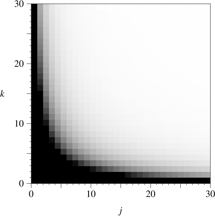
Figure 2: Density plot of the matrix $e_{jk}^{(d)}$, Eq. (31), for $\tau=2.5$, $\kappa=100$, $\kappa^{\prime}=10$. Darker squares represent higher values of $e_{jk}$.

Introducing a cutoff in the degree distribution also provides us with a parameter, namely $\kappa$, that can, as we will shortly see, be conveniently manipulated to produce a phase transition at which a giant component appears in the network.

We can also make an assortative matrix $e_{jk}$ by writing

$$e_{jk}^{(a)}=2q_{j}q_{k}-e_{jk}^{(d)},$$ (34)

which gives a value for the assortativity coefficient of $r_{a}=-r_{d}$, while still having the same degree distribution. More generally, we would like to be able to vary $r$ freely, keeping the degree distribution fixed. We can do this by writing $e_{jk}$ in the form

$$e_{jk}=q_{j}q_{k}+r\sigma_{q}^{2}m_{jk},$$ (35)

where the symmetric matrix $m_{jk}$ has all row and column sums zero and is normalized such that

$$\sum_{jk}jkm_{jk}=1.$$ (36)

For any choice of $m_{jk}$ satisfying these constraints, Eq. (35) gives us a one-parameter family of networks parametrized by the assortativity coefficient $r$. We can for example choose

$$m_{jk}\sim q_{j}q_{k}-e_{jk}^{(d)}=(q_{j}-x_{j})(q_{k}-x_{k}),$$ (37)

for any correctly normalized $x_{k}$. Then Eq. (35) allows us to interpolate smoothly between $e_{jk}^{(d)}$ and $e_{jk}^{(a)}$ (and beyond) by simply varying the value of $r$. Note that whenever $r=0$, we get a simple random graph without degree correlations, of the type discussed by Molloy and Reed MR95 and others .

III.3 Simulation results

For $e_{jk}$ chosen according to Eqs. (35) and (37), with $q_{k}$ and $x_{k}$ taking the same truncated power-law form as in Fig. 2, we have performed simulations for a variety of values of the parameters $\tau$, $\kappa$, and $\kappa^{\prime}$.

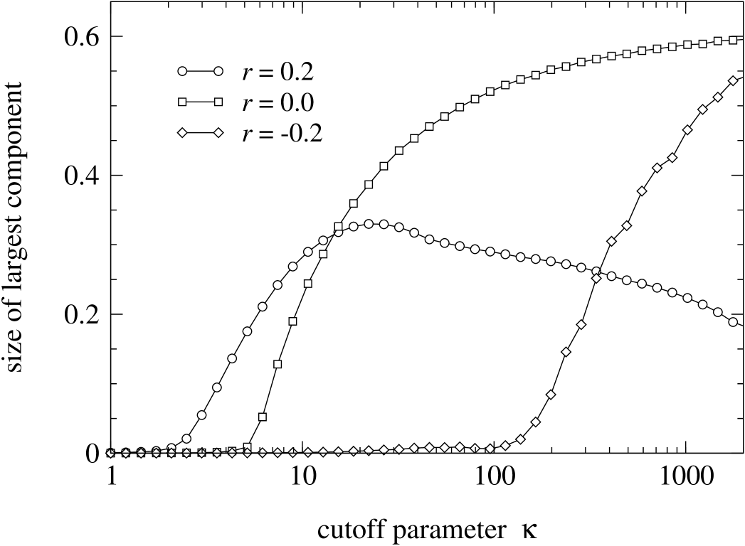
Figure 3: Monte Carlo simulation results for the size of the giant component in graphs with the degree distribution (33), as a function of the cutoff parameter $\kappa$, with $\tau=2.5$ and $\kappa^{\prime}=2$. The individual curves are for different values of the assortativity, as marked. Each data point is an average over 100 graphs of $100\,000$ vertices.

In Fig. 3 we show the size of the largest component in the graph as a function of $\kappa$, for three different values of the assortativity coefficient $r$. As the cutoff parameter $\kappa$ increases, the mean degree of the graph increases also, so that the graph becomes more dense, ultimately passing the critical point at which a giant component develops. The figure reveals two findings of particular note.

1. The position of the phase transition at which the giant component appears moves to higher values of $\kappa$ as the value of $r$ decreases. That is, the more assortative a network is, the lower the edge density at which a giant component first appears. This is intuitively reasonable. In assortatively mixed networks, the high-degree vertices tend to associate preferentially with one another, sticking together and forming what in the epidemiological literature is called a “core group.” Within this core group the edge density is higher than it is in the graph as a whole, since the vertices in the group have higher-than-average degree. Thus one would expect to see a giant-component forming in the core group before it would form in a graph of the same average density but with no assortative mixing. Conversely, in graphs that are disassortatively mixed, the phase transition happens at a higher density than in neutrally mixed graphs.

2. The size of the giant component in the limit of large $\kappa$ is smaller for the assortatively mixed graph than for the neutral and disassortative ones. While this might seem at first to be at odds with the result that assortative graphs show a phase transition at lower density, it is really a reflection of the same underlying mechanism. Although the presence of a core group in an assortative graph allows it to percolate at a lower average density than other graphs, it also means that the density in other parts of the graph, outside the core group, is lower, and hence that the giant component is unlikely to extend into those regions. Thus the giant component is confined to the core of the network, and cannot grow as large as in a neutral or disassortative network.

A question of considerable interest in the study of networked systems is that of network resilience to the deletion of vertices. Suppose vertices are removed one by one from a network. How many must be removed before the giant component of the network is destroyed and network communication between distant vertices can no longer take place? Many networks, particularly those with highly skewed degree distributions, are found to be resilient to the random deletion of vertices but susceptible to the targeted deletion specifically of those vertices that have the highest degrees AJB00 ; Broder00 ; CNSW00 ; CEBH01 . As we now show, these general results are modified by the presence of assortative mixing in the network.

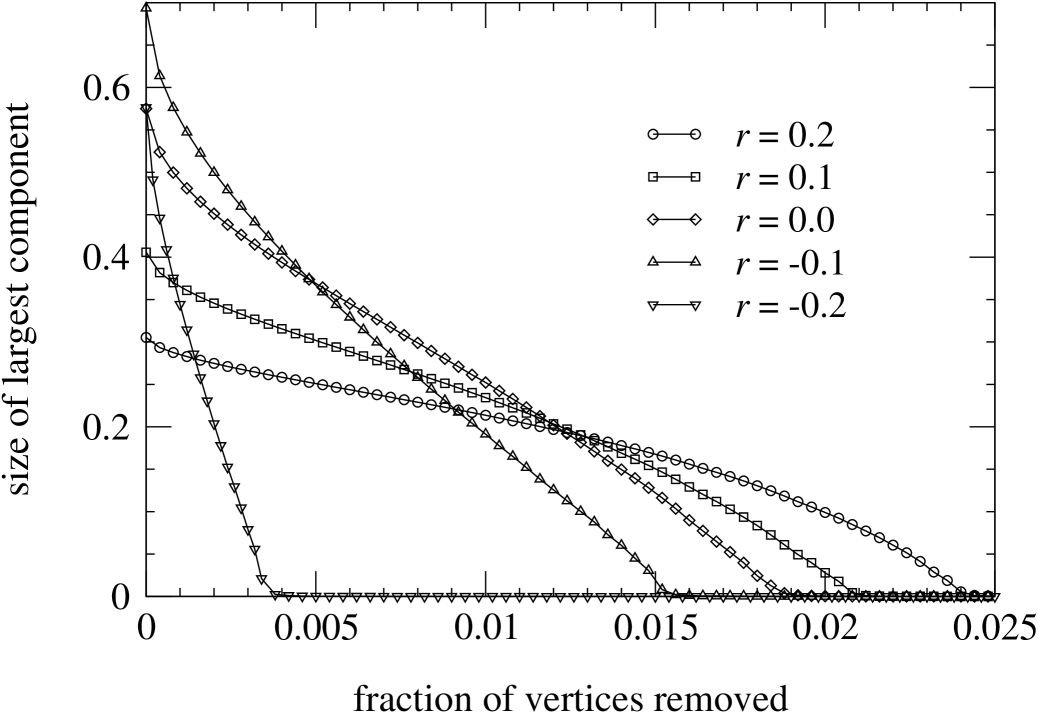
Figure 4: The size of the largest component in a network as a fraction of system size as the highest-degree vertices are removed one by one. Each curve is for a single network of $10^{7}$ vertices generated using the Monte Carlo method described in the text, with the degree distribution and the matrix $e_{jk}$ chosen according to Eqs. (31) and (33), with $\tau=2.5$, $\kappa=500$, $\kappa^{\prime}=5$, and $r$-values as marked. Clearly the most assortatively mixed network ($r=0.2$) is considerably more robust against the removal of vertices than the most disassortative ($r=-0.2$).

In Fig. 4, we show the size of the largest component for five networks with different values of $r$ as vertices are removed in decreasing order of their degree—i.e., highest degree vertices first . As the figure shows, although each of the networks has the same degree distribution, there is dramatic variation in the resilience of the networks with their assortativity. For the most assortative network, with $r=0.2$, it requires the removal of about ten times as many high-degree vertices to destroy the giant component as for the most disassortative one, with $r=-0.2$, even though the disassortative network starts out with a giant component about twice as big.

This finding fits naturally with our picture of an assortative network as dominated by a core group of interconnected high-degree vertices. Such a core group provides robustness to the network by concentrating all the obvious target vertices together in one portion of the graph. Removing these high-degree vertices is still one of the most effective ways to destroy network connectivity, but it is less effective because by removing them all from the same portion of the graph we fail to attack other portions. And if those other portions are themselves percolating, then a giant component will persist even as the highest degree vertices vanish.

Conversely, the disassortatively mixed network is particularly susceptible to removal of high-degree vertices because those vertices are strewn far apart across the network, so that attacking them attacks all parts of the network at once.

One can also ask about the resilience of networks under random failure of their vertices (rather than targeted attack) AJB00 ; CEBH00 ; CNSW00 . Although we do not treat this case in detail here, it is reasonable to suppose that it is similar to the case of targeted attack. If assortative mixing makes networks more resilient against removal of their highest-degree vertices, then presumably they will also be resilient against removal of random ones; random vertex failure will do most damage when it happens to hit high-degree vertices, but, as we have seen, this vulnerability is diminished by the concentration of the high-degree vertices in the core group. Some qualitative behaviors of the system may be unaffected by assortativity, however. For example, it is known that the fraction of vertices that must randomly fail to destroy the giant component in a network with a power-law degree distribution and uncorrelated degrees tends to unity as graph size becomes large, provided the exponent of the power law satisfies $\tau<3$ CEBH00 . Vazquez and Moreno VM03 have recently shown that this result is not affected by the presence of assortative mixing by degree in the network, although disassortative mixing can make a difference.

III.4 Discussion

The results found here could have applications in a variety of areas. Consider for example, the spread of diseases on networks, which has been the subject of much attention in the recent networks literature BMS97 ; Andersson99 ; MN00a ; PV01a ; PV01b ; ML01 ; Sander02 ; Newman02c . The largest component of the contact network over which a disease spreads represents the largest possible disease outbreak on that network, and a network with no giant component cannot show an epidemic (system-wide) outbreak. Thus our finding that a giant component forms more easily in a network that is assortatively mixed by degree suggests that in such networks epidemic outbreaks would become possible at a lower edge density than in the corresponding disassortative network. In the language of epidemiology, the core group of an assortatively mixed network forms a “reservoir,” which can sustain an outbreak of the disease even when the density of the network as a whole is too low to do so. On the other hand, the smaller asymptotic size of the giant component in an assortatively mixed network seems to imply that, when they occur, epidemics in such networks would be restricted to a smaller segment of the population than in a similar disassortative network—the outbreak is confined mostly to the core group and does not spread to the population as a whole. Thus from the epidemiological point of view there are both good and bad sides to the phenomenon of assortativity.

One could test these predictions explicitly by studying epidemic models such as SIR or SIRS models Bailey75 ; Hethcote00 on assortatively mixed model networks of the type introduced here. Some studies of this kind have already been carried out—see for example Refs. BPV02, and MV03, —although the particular conjectures put forward here have not been conclusively verified.

Our findings on network resilience also have some practical implications. In the context of epidemiology, for instance, removal of vertices from the network might correspond to immunization of individuals to prevent the spread of disease. Assuming that the goal of a vaccination program is to destroy network connectivity so that the disease in question cannot spread, our findings suggest that even targeted vaccination strategies would be less effective in assortative networks than in disassortative or neutral ones because of the resilience of the network to this type of attack. In other contexts, however, resilience is a good thing. For example we would like to make networks such as the Internet and other communication or distribution networks resilient against attacks on their vertices. In this context assortative mixing would be beneficial.

Unfortunately, when we look at Table 2, we find a discouraging picture. As we pointed out in Section III.1, almost all the social networks we have looked at are significantly assortative, meaning that they would be robust to vertex removal. But these are the very networks by which disease spreads, the ones that we would like to be able to attack using vaccination strategies. Even the email network, which is relevant to the spread of computer viruses NFB02 , is assortative and hence resilient. On the other hand, the technological networks like the Internet, which we would like to be able to protect, are disassortative, and hence particularly vulnerable to targeted attack.

IV Conclusions

In this paper we have studied the phenomenon of assortative mixing in networks, which is the tendency for vertices in networks to connect preferentially to other vertices that are like them in some way. This preference may take a number of forms. Mixing may follow discrete or enumerative characteristics. In the social networks that have been the main focus of this paper, connections between people may be assortative by language, for example, or by race—people may prefer to associate with others who speak the same language as they do or are of the same race. Mixing can also be dictated by scalar characteristics such as age or income. A special case of mixing by a scalar characteristic is mixing according to vertex degree, which has been shown previously to be present in a variety of networks, including non-social ones such as the Internet and protein interaction networks. Mixing can also be disassortative, meaning that vertices in the network preferentially form connections to others that are unlike them.

We have proposed some simple measures for these types of mixing, which we call assortativity coefficients. These measures are positive or negative for assortative or disassortative mixing respectively, and zero for neutrally mixed networks. Applying our measures to a broad selection of network data drawn from various real-world situations we have shown that the phenomenon of assortative mixing is indeed widespread, with only a few of the networks studied showing no statistically significant biases in their mixing patterns. In the case of mixing by vertex degree, a remarkable pattern emerges. Almost all the social networks studied show positive assortativity coefficients while all other types of networks, including technological and biological networks, show negative coefficients, i.e., disassortative mixing. Only three networks that showed no significant trend either way failed to follow this rule. We have offered some conjectures about the origin of this striking regularity, but we believe it unlikely that any single mechanism can explain the mixing patterns of all of these disparate networks.

We have also proposed a number of models of assortatively mixed networks, for mixing both by discrete and by scalar characteristics. For each of the mixing types considered it is possible to create random graph models for which one can calculate exactly by generating function methods certain average properties of network ensembles. We have also described Monte Carlo methods for generating random graphs drawn from each of the classes discussed with specified values of the mixing parameters.

For the case of mixing by vertex degree we have performed extensive simulations. Two results of particular interest emerge from these studies. First, we find that networks that are assortatively mixed by degree percolate more easily that their disassortative counterparts. That is, a giant component of connected vertices forms in the network at lower edge density than in another network with the same degree distribution but zero or negative assortativity. This result may imply, for instance, that assortatively mixed social networks would support epidemic disease outbreaks more easily than disassortatively mixed ones, which would be a disheartening conclusion, given our finding that most social networks appear to be assortative.

Second, we find that assortatively mixed networks are more robust to the deletion of their vertices than disassortatively mixed or neutral networks. We have studied in particular the case of the targeted deletion of the highest-degree vertices, which has been suggested as a possible vaccination strategy for breaking up networks of disease-causing contacts, but it is reasonable to suppose that the same result will extend also to the random deletion of vertices. This result too leads to a rather gloomy conclusion: targeted vaccination strategies may be less effective than we would hope in preventing disease because of the assortative and hence resilient nature of social networks, while on the other hand networks that we would hope to protect against vertex removal, communication networks like the Internet, for instance, will be particularly susceptible because of their disassortative nature.

Appendix A The assortativity measure of Gupta et al.

Gupta et al. GAM89 have defined a measure of assortative mixing by discrete types different from the one that we have introduced in Section II.1. In our notation their measure is

$$Q={\sum_{i}a_{i}^{-1}(e_{ii}-a_{i}b_{i})\over n-1}={\sum_{i}e_{ii}/a_{i}-1\over n-1},$$ (38)

where as before $n$ is the number of vertex types, and we have made use of $\sum_{i}b_{i}=1$. Like our measure, this measure is 0 for a neutrally mixed network and 1 for a perfectly assortative network. In general, however, the values of the two measures are quite different. Here we give a simple example to illustrate the difference between the two.

Consider a network with three types of vertices. There are 100 vertices of type 1, 100 of type 2, and 2 of type 3. The vertices of types 1 and 2 mix indiscriminately with one other—connections from 1 to 2 are as likely as from 1 to 1, and so forth. The vertices of type 3 however associate only among themselves and not with types 1 and 2 at all. This is reflected in the matrix $\mathbf{e}$ for the 202 vertices, which for a network with mean degree 2 would look like this:

$$\mathbf{e}={1\over 202}\begin{pmatrix}50&50&0\\ 50&50&0\\ 0&0&2\\ \end{pmatrix}.$$ (39)

Clearly most of this network—99% of it, in fact—is mixing randomly, and hence we would expect the assortativity coefficient to be close to zero. The value of $r$ for the matrix above reflects this; we find $r=0.029$. The measure of Gupta et al. GAM89 , however, takes a value $Q=0.50$. This appears to indicate that the network has very strong assortative mixing, when in fact it does not. The reason for this is that the measure of Gupta et al., rather than giving each vertex in the network equal weight, weights each type of vertex equally, so that vertices that belong to large groups get less weight in the calculation than those in small groups. In the present case, where one group is very small, the vertices in that group are weighted very heavily, and since those vertices mix perfectly assortatively, the value of $Q$ is, as a result, high. If we remove these vertices from the network, the value of Gupta et al.’s $Q$ coefficient jumps to zero. Thus the two vertices in the third group have a disproportionately large effect on the value of $Q$.

The solution to this problem is to give each vertex equal weight in the calculation, which is precisely what our measure $r$ does.

References

- (1) S. H. Strogatz, Exploring complex networks. Nature 410, 268–276 (2001).
- (2) R. Albert and A.-L. Barabási, Statistical mechanics of complex networks. Rev. Mod. Phys. 74, 47–97 (2002).
- (3) S. N. Dorogovtsev and J. F. F. Mendes, Evolution of networks. Advances in Physics 51, 1079–1187 (2002).
- (4) J. Travers and S. Milgram, An experimental study of the small world problem. Sociometry 32, 425–443 (1969).
- (5) D. J. Watts and S. H. Strogatz, Collective dynamics of ‘small-world’ networks. Nature 393, 440–442 (1998).
- (6) A.-L. Barabási and R. Albert, Emergence of scaling in random networks. Science 286, 509–512 (1999).
- (7) L. A. N. Amaral, A. Scala, M. Barthélémy, and H. E. Stanley, Classes of small-world networks. Proc. Natl. Acad. Sci. USA 97, 11149–11152 (2000).
- (8) R. Albert, H. Jeong, and A.-L. Barabási, Attack and error tolerance of complex networks. Nature 406, 378–382 (2000).
- (9) A. Broder, R. Kumar, F. Maghoul, P. Raghavan, S. Rajagopalan, R. Stata, A. Tomkins, and J. Wiener, Graph structure in the web. Computer Networks 33, 309–320 (2000).
- (10) R. Cohen, K. Erez, D. ben-Avraham, and S. Havlin, Resilience of the Internet to random breakdowns. Phys. Rev. Lett. 85, 4626–4628 (2000).
- (11) D. S. Callaway, M. E. J. Newman, S. H. Strogatz, and D. J. Watts, Network robustness and fragility: Percolation on random graphs. Phys. Rev. Lett. 85, 5468–5471 (2000).
- (12) P. Holme, B. J. Kim, C. N. Yoon, and S. K. Han, Attack vulnerability of complex networks. Phys. Rev. E 65, 056109 (2002).
- (13) J. M. Kleinberg, The small-world phenomenon: An algorithmic perspective. In Proceedings of the 32nd Annual ACM Symposium on Theory of Computing, pp. 163–170, Association of Computing Machinery, New York (2000).
- (14) L. A. Adamic, R. M. Lukose, A. R. Puniyani, and B. A. Huberman, Search in power-law networks. Phys. Rev. E 64, 046135 (2001).
- (15) D. J. Watts, P. S. Dodds, and M. E. J. Newman, Identity and search in social networks. Science 296, 1302–1305 (2002).
- (16) M. Girvan and M. E. J. Newman, Community structure in social and biological networks. Proc. Natl. Acad. Sci. USA 99, 8271–8276 (2002).
- (17) P. Holme, M. Huss, and H. Jeong, Subnetwork hierarchies of biochemical pathways. Preprint cond-mat/0206292 (2002).
- (18) R. Guimerà, L. Danon, A. Díaz-Guilera, F. Giralt, and A. Arenas, Self-similar community structure in organisations. Preprint cond-mat/0211498 (2002).
- (19) R. Monasson, Diffusion, localization and dispersion relations on ‘small-world’ lattices. Eur. Phys. J. B 12, 555–567 (1999).
- (20) K.-I. Goh, B. Kahng, and D. Kim, Spectra and eigenvectors of scale-free networks. Phys. Rev. E 64, 051903 (2001).
- (21) I. J. Farkas, I. Derényi, A.-L. Barabási, and T. Vicsek, Spectra of “real-world” graphs: Beyond the semicircle law. Phys. Rev. E 64, 026704 (2001).
- (22) M. E. J. Newman, Assortative mixing in networks. Phys. Rev. Lett. 89, 208701 (2002).
- (23) J. A. Catania, T. J. Coates, S. Kegels, and M. T. Fullilove, The population-based AMEN (AIDS in Multi-Ethnic Neighborhoods) study. Am. J. Public Health 82, 284–287 (1992).
- (24) M. Morris, Data driven network models for the spread of infectious disease. In D. Mollison (ed.), Epidemic Models: Their Structure and Relation to Data, pp. 302–322, Cambridge University Press, Cambridge (1995).
- (25) S. Gupta, R. M. Anderson, and R. M. May, Networks of sexual contacts: Implications for the pattern of spread of HIV. AIDS 3, 807–817 (1989).
- (26) B. Efron, Computers and the theory of statistics: Thinking the unthinkable. SIAM Review 21, 460–480 (1979).
- (27) J. L. Fleiss, Statistical Methods for Rates and Proportions. John Wiley, New York (1981).
- (28) J. L. Fleiss, J. Cohen, and B. S. Everitt, Large sample standard errors of kappa and weighted kappa. Psychol. Bull. 72, 323–327 (1969).
- (29) E. A. Bender and E. R. Canfield, The asymptotic number of labeled graphs with given degree sequences. Journal of Combinatorial Theory A 24, 296–307 (1978).
- (30) T. Łuczak, Sparse random graphs with a given degree sequence. In A. M. Frieze and T. Łuczak (eds.), Proceedings of the Symposium on Random Graphs, Poznań 1989, pp. 165–182, John Wiley, New York (1992).
- (31) M. Molloy and B. Reed, A critical point for random graphs with a given degree sequence. Random Structures and Algorithms 6, 161–179 (1995).
- (32) M. Molloy and B. Reed, The size of the giant component of a random graph with a given degree sequence. Combinatorics, Probability and Computing 7, 295–305 (1998).
- (33) W. Aiello, F. Chung, and L. Lu, A random graph model for massive graphs. In Proceedings of the 32nd Annual ACM Symposium on Theory of Computing, pp. 171–180, Association of Computing Machinery, New York (2000).
- (34) M. E. J. Newman, S. H. Strogatz, and D. J. Watts, Random graphs with arbitrary degree distributions and their applications. Phys. Rev. E 64, 026118 (2001).
- (35) M. E. J. Newman, D. J. Watts, and S. H. Strogatz, Random graph models of social networks. Proc. Natl. Acad. Sci. USA 99, 2566–2572 (2002).
- (36) M. E. J. Newman and G. T. Barkema, Monte Carlo Methods in Statistical Physics. Oxford University Press, Oxford (1999).
- (37) National Survey of Family Growth, Cycle V, 1995. U.S. Department of Health and Human Services, National Center for Health Statistics, Hyattsville, MD (1997).
- (38) R. Pastor-Satorras, A. Vázquez, and A. Vespignani, Dynamical and correlation properties of the Internet. Phys. Rev. Lett. 87, 258701 (2001).
- (39) J. M. Montoya and R. V. Solé, Small world patterns in food webs. J. Theor. Bio. 214, 405–412 (2002).
- (40) S. N. Dorogovtsev, J. F. F. Mendes, and A. N. Samukhin, Modern architecture of random graphs: Constructions and correlations. Preprint cond-mat/0206467 (2002).
- (41) A. Vázquez and M. Weigt, Computational complexity arising from degree correlations in networks. Preprint cond-mat/0207035 (2002).
- (42) M. Boguñá, R. Pastor-Satorras, and A. Vespignani, Absence of epidemic threshold in scale-free networks with connectivity correlations. Preprint cond-mat/0208163 (2002).
- (43) M. E. J. Newman, The structure of scientific collaboration networks. Proc. Natl. Acad. Sci. USA 98, 404–409 (2001).
- (44) J. W. Grossman and P. D. F. Ion, On a portion of the well-known collaboration graph. Congressus Numerantium 108, 129–131 (1995).
- (45) G. F. Davis, M. Yoo, and W. E. Baker, The small world of the corporate elite. Preprint, University of Michigan Business School (2001).
- (46) P. S. Bearman, J. Moody, and K. Stovel, Chains of affection: The structure of adolescent romantic and sexual networks. Preprint, Department of Sociology, Columbia University (2002).
- (47) M. E. J. Newman, S. Forrest, and J. Balthrop, Email networks and the spread of computer viruses. Phys. Rev. E 66, 035101 (2002).
- (48) Q. Chen, H. Chang, R. Govindan, S. Jamin, S. J. Shenker, and W. Willinger, The origin of power laws in Internet topologies revisited. In Proceedings of the 21st Annual Joint Conference of the IEEE Computer and Communications Societies, IEEE Computer Society (2002).
- (49) R. Albert, H. Jeong, and A.-L. Barabási, Diameter of the world-wide web. Nature 401, 130–131 (1999).
- (50) H. Jeong, S. Mason, A.-L. Barabási, and Z. N. Oltvai, Lethality and centrality in protein networks. Nature 411, 41–42 (2001).
- (51) H. Jeong, B. Tombor, R. Albert, Z. N. Oltvai, and A.-L. Barabási, The large-scale organization of metabolic networks. Nature 407, 651–654 (2000).
- (52) J. G. White, E. Southgate, J. N. Thompson, and S. Brenner, The structure of the nervous system of the nematode C. Elegans. Phil. Trans. R. Soc. London 314, 1–340 (1986).
- (53) M. Huxham, S. Beaney, and D. Raffaelli, Do parasites reduce the chances of triangulation in a real food web? Oikos 76, 284–300 (1996).
- (54) N. D. Martinez, Artifacts or attributes? Effects of resolution on the Little Rock Lake food web. Ecological Monographs 61, 367–392 (1991).
- (55) D. Strauss, On a general class of models for interaction. SIAM Review 28, 513–527 (1986).
- (56) T. A. B. Snijders, Markov chain Monte Carlo estimation of exponential random graph models. Journal of Social Structure 2(2) (2002).
- (57) D. J. de S. Price, Networks of scientific papers. Science 149, 510–515 (1965).
- (58) S. Redner, How popular is your paper? An empirical study of the citation distribution. Eur. Phys. J. B 4, 131–134 (1998).
- (59) M. Faloutsos, P. Faloutsos, and C. Faloutsos, On power-law relationships of the internet topology. Computer Communications Review 29, 251–262 (1999).
- (60) F. Liljeros, C. R. Edling, L. A. N. Amaral, H. E. Stanley, and Y. Åberg, The web of human sexual contacts. Nature 411, 907–908 (2001).
- (61) H. Ebel, L.-I. Mielsch, and S. Bornholdt, Scale-free topology of e-mail networks. Phys. Rev. E 66, 035103 (2002).
- (62) R. Cohen, K. Erez, D. ben-Avraham, and S. Havlin, Breakdown of the Internet under intentional attack. Phys. Rev. Lett. 86, 3682–3685 (2001).
- (63) A. Vázquez and Y. Moreno, Resilience to damage of graphs with degree correlations. Phys. Rev. E 67, 015101 (2003).
- (64) F. Ball, D. Mollison, and G. Scalia-Tomba, Epidemics with two levels of mixing. Annals of Applied Probability 7, 46–89 (1997).
- (65) H. Andersson, Epidemic models and social networks. Math. Scientist 24, 128–147 (1999).
- (66) C. Moore and M. E. J. Newman, Epidemics and percolation in small-world networks. Phys. Rev. E 61, 5678–5682 (2000).
- (67) R. Pastor-Satorras and A. Vespignani, Epidemic spreading in scale-free networks. Phys. Rev. Lett. 86, 3200–3203 (2001).
- (68) R. Pastor-Satorras and A. Vespignani, Epidemic dynamics and endemic states in complex networks. Phys. Rev. E 63, 066117 (2001).
- (69) R. M. May and A. L. Lloyd, Infection dynamics on scale-free networks. Phys. Rev. E 64, 066112 (2001).
- (70) L. M. Sander, C. P. Warren, I. Sokolov, C. Simon, and J. Koopman, Percolation on disordered networks as a model for epidemics. Math. Biosci. 180, 293–305 (2002).
- (71) M. E. J. Newman, Spread of epidemic disease on networks. Phys. Rev. E 66, 016128 (2002).
- (72) N. T. J. Bailey, The Mathematical Theory of Infectious Diseases and its Applications. Hafner Press, New York (1975).
- (73) H. W. Hethcote, Mathematics of infectious diseases. SIAM Review 42, 599–653 (2000).
- (74) Y. Moreno and A. Vázquez, Disease spreading in structured scale-free networks. Preprint cond-mat/0210362 (2002).