[

Quantum behavior of Orbitals in Ferromagnetic Titanates:
Novel Orderings and Excitations

Abstract

We investigate the collective behavior of orbital angular momentum in the spin ferromagnetic state of a Mott insulator with $t_{2g}$ orbital degeneracy. The frustrated nature of the interactions leads to an infinite degeneracy of classical states. Quantum effects select four distinct orbital orderings. Two of them have a quadrupolar order, while the other states show in addition weak orbital magnetism. Specific predictions are made for neutron scattering experiments which might help to identify the orbital order in YTiO₃ and to detect the elementary orbital excitations.

]

Recently, “orbital physics” has become an important topic in the physics of transition metal oxides[1, 2]. Orbital degeneracy of low energy states and the extreme sensitivity of the magnetic bonds to the spatial orientation of orbitals lead to a variety of competing phases that are tunable by a moderate external fields. A well known example is “colossal magnetoresistivity” of manganites. A “standard” view on orbital physics is based on pioneering works[3, 4], developed and summarized in Ref.[5]. In this picture, long-range coherence of orbitals sets in below a cooperative orbital/Jahn-Teller (JT) transition; spin interactions on every bond are then fixed by the Goodenough-Kanamori rules. Implicit in this picture is that the orbital splittings are large enough so that one can consider orbital populations as classical numbers. Such a classical treatment of orbitals is well justified when orbital order is driven by strong cooperative lattice distortion.

However, interesting quantum effects are expected to come into play when orbital physics is dominated by electronic correlations. Mott insulators with threefold $t_{2g}$ degeneracy (titanates, vanadates) are of particular interest in this respect, as the relative weakness of the JT coupling for $t_{2g}$ orbitals and their large degeneracy enhance quantum effects. A picture of strongly fluctuating orbitals in titanate LaTiO₃ has recently been proposed on both experimental[6] and theoretical grounds [7, 8].

Titanates are very interesting: they show a nearly continuous transition from an antiferromagnetic state in LaTiO₃ with unusually small moment to a saturated ferromagnetic one in YTiO₃ [9]. Yet another puzzle is the almost gapless spinwave spectrum of cubic symmetry recently observed in YTiO₃ by Ulrich et al. [10]. This finding is striking, because the orbital state predicted by band structure calculations [11] is expected to break cubic symmetry of the spin couplings. In principle, one may obtain isotropic spin exchange couplings by using this orbital state [12]; however, this requires fine tuning of parameters, and rather small changes of the orbital state may reverse even the sign of the spin couplings [10].

To gain more insight into the origin of the different behavior of orbitals in YTiO₃ and LaTiO₃, we ask in this Letter the following question: What kind of orbital state would optimize the superexchange (SE) energy if we fix the spin state to be ferromagnetic as in YTiO₃? We find a surprisingly rich physics: (i) there are several “best” orderings, some of them are highly unusual showing static orbital magnetism; (ii) the resulting spin interactions respect cubic symmetry in accord with experimental data; (iii) strong orbital fluctuations lead to anomalously large order parameter reduction. These states have been overlooked previously, as their stabilization is an effect of quantum origin. We also discuss a mechanism which stabilizes ferromagnetic state in YTiO₃.

The $t_{2g}$ superexchange can, in general, be written as $H_{SE}=J_{SE}\sum_{\langle ij\rangle}\bigl{[}\bigl{(}{\vec{S}}_{i}\cdot{\vec{S}}_{j}+\frac{1}{4}\bigl{)}\hat{J}_{ij}^{(\gamma)}~{}+~{}\frac{1}{2}\hat{K}_{ij}^{(\gamma)}\bigl{]}$, where $J_{SE}=4t^{2}/U$ represents the overall energy scale. The orbital operators $\hat{J}_{ij}^{(\gamma)}$ and $\hat{K}_{ij}^{(\gamma)}$ depend on bond directions $\gamma(=a,b,c)$. Their explicit form in a $d^{1}(t_{2g})$ system like the titanates is given in Ref.[8]. If spins are all aligned ferromagnetically (i.e., ${\vec{S}}_{i}\cdot{\vec{S}}_{j}=1/4$), the above equation reduces to the orbital Hamiltonian:

$$H_{orb}=\frac{1}{2}\sum_{\langle ij\rangle}A_{ij}^{(\gamma)}.$$ (1)

Hereafter, we use $r_{1}J_{SE}$ as a unit of energy and drop a constant energy shift ($=-r_{1}J_{SE}$). The coefficient $r_{1}=1/(1-3\eta)$ originates from Hund’s splitting of the excited $t_{2g}^{2}$ multiplet via $\eta=J_{H}/U$. The orbital operators $A_{ij}^{(\gamma)}$ can be represented via a triplet ${\bf t}_{i}=(a,b,c)_{i}$ of constrained particles ($n_{ia}+n_{ib}+n_{ic}=1$) corresponding to $t_{2g}$ levels of $yz$, $xz$, $xy$ symmetry, respectively. Namely,

$$A_{ij}^{(c)}=n_{ia}n_{ja}+n_{ib}n_{jb}+a_{i}^{\dagger}b_{i}b_{j}^{\dagger}a_{j}+b_{i}^{\dagger}a_{i}a_{j}^{\dagger}b_{j},$$ (2)

for the pair along the $c$ axis. Similar expressions are obtained for the exchange bonds along the $a$ and $b$ axes by using in Eq. (2) $(b,c)$ and $(c,a)$ orbiton doublets, respectively. The Hamiltonian (1) is the main focus of this Letter; a theory of ferromagnetic magnons including spin-orbital effects will be presented in Ref.[13].

FIG. 1.: Arrangement of the local quantization axes in states (a) and (b). Each state has four sublattices denoted by numbers. Arrows show a direction of the quantization axes at each site. They represent also a snapshot of local correlations of orbital angular momentum: on every bond, two out of three components $l_{\alpha}$ are correlated antiferromagnetically.

It is useful to look at the structure of $H_{orb}$ from different points of view (see also Refs.[7, 8, 14]): (i) On a given bond, the operator $A_{ij}^{(\gamma)}$ acts within a particular doublet of orbitals. Spinlike physics, that is, the formation of orbital singlets, is therefore possible. This is the origin of orbital fluctuations in titanates. (ii) On the other hand, interactions on different bonds are competing: they involve different doublets, thus frustrating each other. This brings about a Potts model like frustrations, from which the high degeneracy of classical orbital configurations follows. (iii) Finally, using the angular momentum operators $l_{x}=i(c^{\dagger}b-b^{\dagger}c)$ , $l_{y}=i(a^{\dagger}c-c^{\dagger}a)$ , $l_{z}=i(b^{\dagger}a-a^{\dagger}b)$ of $t_{2g}$ level, one may represent the interaction as follows:

$$A_{ij}^{(c)} = (1-l_{x}^{2})_{i}(1-l_{x}^{2})_{j}+(1-l_{y}^{2})_{i}(1-l_{y}^{2})_{j}$$ (4)

$$+(l_{x}l_{y})_{i}(l_{y}l_{x})_{j}+(l_{y}l_{x})_{i}(l_{x}l_{y})_{j}~{}.$$

(For $b$ and $a$ bonds, the interactions are obtained by permutations of $l_{z},l_{y},l_{x}$.) We observe a pseudospin $l=1$ interaction of pure biquadratic form. Would $\vec{l}$ be a classical vector, it could change its sign at any site independently. A local “$Z_{2}$ symmetry” and the associated degeneracy of the classical states tells us that angular momentum ordering, if any, is of pure quantum origin.

The above points (i)$-$(iii) govern the underlying physics of the orbital Hamiltonian. By inspection of the global structure of $A_{ij}^{(\gamma)}$, one observes that the first two terms are definitely positive. However, the last two terms (which change the “color” of orbitals) can be made negative on all the bonds simultaneously, if (i) on every bond, two particular components of $\vec{l}_{i}$ and $\vec{l}_{j}$ are antiparallel, and (ii) remaining third components are parallel. For $c$ bonds the rule reads as: $l_{iz}l_{jz}$ and $l_{ix}l_{jx}$ are both negative, while $l_{y}$ components are parallel. (In terms of orbitons: $c_{i}$ and $c_{j}$ are in antiphase, $a_{i}$ and $a_{j}$ as well; but $b_{i}$ and $b_{j}$ have the same phase.) We find only two topologically different arrangements [called (a) and (b)], which can accommodate this curious mixture of “2/3 antiferro” plus “1/3 ferro” correlations (see Fig.1).

For technical reasons, and also to simplify a physical picture, it is useful to introduce new quantization axes. This is done in two steps. First, we introduce local, sublattice specified quantization axes (see Fig.1):

$$1 : (x,y,z)\rightarrow(x,y,z),\hskip 20.00003pt2:(x,y,z)\rightarrow(-x,-y,z),$$ (5)

$$3 : (x,y,z)\rightarrow(-x,y,-z),\hskip 5.0pt4:(x,y,z)\rightarrow(x,-y,-z).$$ (6)

After corresponding sign transformations of $l_{i\alpha}$ and orbitons, one obtains a negative sign in front of the last two terms of $A_{ij}^{(\gamma)}$, thereby “converting” the interactions in a new axes to a fully ferromagnetic one. From now on, a sublattice structure will not enter in the excitation spectrum. From the above observations, it is also clear that all the components of $\vec{l}$ are equally needed to optimize all three directions. We anticipate, therefore, that the cubic diagonals are “easy” (or “hard”) axis for $\vec{l}$ fluctuations/orderings (recall that the Hamiltonian has no rotational symmetry). The second step is then to rotate quantization axes so that the new $z$ axis ($\tilde{z}$) is along one of the cubic diagonals (say, $[111]$). This is done as follows: $\vec{l}_{i}=\hat{R}~{}\vec{\tilde{l}}_{i}$ (and ${\bf t}=\hat{R}~{}\tilde{\bf t}$ for orbitons). The matrix $\hat{R}=\hat{R}_{z}(\pi/4)\hat{R}_{y}(\theta_{0})\hat{R}_{z}(-\pi/4)$ with $\tan\theta_{0}=\sqrt{2}$. $\hat{R}_{\alpha}(\theta)$ describes the rotation around $\alpha$ axis by angle $\theta$.

By the above transformations, the orbital Hamiltonian obtains well structured form and can be divided into two parts as $\tilde{H}_{orb}=H_{Ising}+H_{trans}$. Here, $H_{Ising}$ represents a “longitudinal” part of the interaction:

$$H_{Ising}=\frac{1}{6}\sum_{\langle ij\rangle}\Bigl{[}\tilde{l}_{iz}^{2}+\tilde{l}_{jz}^{2}-\frac{3}{2}\tilde{l}_{iz}^{2}\tilde{l}_{jz}^{2}-\frac{1}{2}\tilde{l}_{iz}\tilde{l}_{jz}\Bigr{]}.$$ (7)

$H_{trans}$ is responsible for fluctuations of transverse components $\tilde{l}_{x}$, $\tilde{l}_{y}$ and quadrupole moments of various symmetry. Its explicit, somewhat lengthy form will be presented in Ref.[13]. In terms of $\tilde{a}$, $\tilde{b}$, $\tilde{c}$ orbitons, $H_{Ising}$ promotes a condensation of an appropriate orbiton, while $H_{trans}$ gives a dispersion of orbitons and their interactions.

Order and excitations.—Now we are ready to discuss possible orbital orderings. Equation (7) makes it explicit that there are two deep classical minima corresponding to two different “ferro-type” states: (I) quadrupole ordering (classically, $l_{iz}=0$) and (II) magnetic ordering ($l_{iz}=1$, classically). We notice that the last, magnetic term in Eq. (7) is generated by quantum commutation rules when we rotate $H_{orb}$; this makes explicit that the $Z_{2}$ symmetry is only a classical one and emphasizes the quantum origin of orbital magnetism. We see below that states I and II are degenerate even on a quantum level. Noticing that an arbitrary cubic diagonal could be taken as $\tilde{z}$ and having in mind also two structures in Fig.1, one obtains a multitude of degenerate states. This makes, in fact, all the orderings very fragile.

To be more specific about the last statement, we calculate the excitation spectrum. Introduce first a quadrupole order parameter $Q=\langle(\tilde{l}_{x}^{2}+\tilde{l}_{y}^{2})/2-\tilde{l}_{z}^{2}\rangle=\langle n_{\tilde{c}}-(n_{\tilde{a}}+n_{\tilde{b}})/2\rangle$, and the magnetic moment $m_{l}=\langle\tilde{l}_{z}\rangle=i\langle\tilde{b}^{\dagger}\tilde{a}-\tilde{a}^{\dagger}\tilde{b}\rangle$ (we set $\mu_{B}=1$). State I corresponds to the condensation of the orbital $\tilde{c}$ (an equal mixture of the original $a,b,c$ states), while the ordering orbital in the state II is an imaginary one $(\tilde{a}-i\tilde{b})/\sqrt{2}$. Let us call the remaining two orbitals by $\alpha$ and $\beta$, which are the excitations of the model. Specifically, $\alpha=\tilde{a}$, $\beta=\tilde{b}$ in state I, and $\alpha=[\tilde{a}+i\tilde{b}+(1+i)\tilde{c}]/2$, $\beta=[\tilde{b}-i\tilde{a}-(1-i)\tilde{c}]/2$ in state II. Note that latter doublets can be regarded as magnons of orbital origin, describing fluctuations of the orbital magnetism. Remarkably, in terms of these doublet excitations, the linearized Hamiltonian in a momentum space has the same form for both phases. Namely,

$$H_{OW} = \textstyle{\sum_{\vec{k}}\Bigl{[}n_{\alpha\vec{k}}+n_{\beta\vec{k}}+\Bigl{\{}\frac{1}{2}(\gamma_{1}+\gamma_{2})\alpha_{\vec{k}}\alpha_{-\vec{k}}}$$ (9)

$$\hskip 16.99998pt\textstyle{+\frac{1}{2}(\gamma_{1}-\gamma_{2})\beta_{\vec{k}}\beta_{-\vec{k}}-\gamma_{3}\alpha_{\vec{k}}\beta_{-\vec{k}}+H.c.\Bigr{\}}\Bigr{]},}$$

where $\gamma_{1}=(c_{x}+c_{y}+c_{z})/3$, $\gamma_{2}=\sqrt{3}(c_{y}-c_{x})/6$, $\gamma_{3}=(2c_{z}-c_{x}-c_{y})/6$, and $c_{\alpha}=\cos k_{\alpha}$. These expressions refer to state I. For state II, one should just interchange $\gamma_{2}$ and $\gamma_{3}$. However this does not affect the spectrum of the elementary excitations, which is given by $\omega_{\pm}(\vec{k})=\sqrt{1-(\gamma_{1}\pm\kappa)^{2}}$, where $\kappa=\sqrt{\gamma_{2}^{2}+\gamma_{3}^{2}}$.

Using matrix Green’s functions for the ($\alpha,\beta$) doublet, we may calculate various expectation values: (i) quantum energy gain: $E_{0}=-0.214$ for all the phases; (ii) number of bosons not in the condensate: $\langle n_{\alpha}+n_{\beta}\rangle=0.54$. Thus, the order parameters are strongly reduced by fluctuations. We obtain $Q=0.19$ ($m_{l}=0$, of course) in state I, and $m_{l}=0.19$ accompanied with small quadrupole moment $Q=-0.095$ in state II. To visualize the orbital patterns, we show in Fig. 2 the electron density calculated including quantum fluctuations.

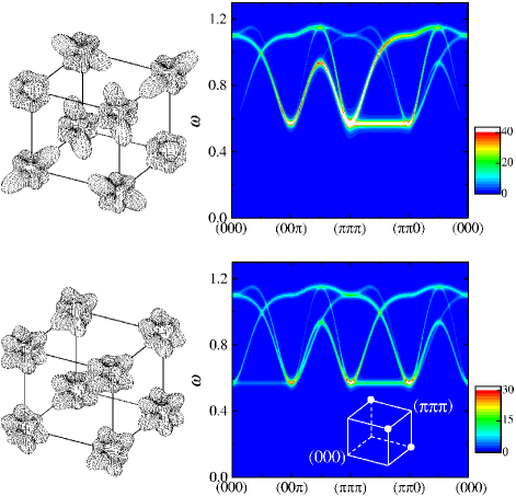
FIG. 2.: $t_{2g}$ electron density (left) and intensity of the orbital contribution to the structure factor $S(\vec{q},\omega)$ (right). Upper panel: Quadrupole ordered state I (a). Because of the more spatial anisotropy of electron distribution, this state may be preferred by electron-lattice coupling. “Hot spot” at ($\pi,\pi,\pi$) point is due to coherency factors stemming from four sublattice structure. Lower panel: Magnetic state II (a). Shown in the inset are the expected orbital Bragg peak positions.

The anomalous reduction of order parameters is due to the highly frustrated nature of the interactions in Eq. (1). A special, nonspinlike feature of all orbital models is that orbitals are bond selective, resulting in a pathological degeneracy of classical states. This leads to soft modes [observe that $\omega_{\pm}(\vec{k})$ is just flat along ($0,0,\pi$) and equivalent directions]; such soft modes were first noticed in Ref.[15]. Linear, “spin-wave-like” modes are, however, not true eigenstates even in the small momentum limit, as orbital models have no continuous symmetry. Therefore, an orbital gap must appear (see Ref. [16] and, in particular, the discussion of the “cubic” model in Ref. [8]). In the present model, we have estimated the orbital gap $\Delta=0.57$ using a single mode approximation [17].

Angular momentum fluctuations can directly be probed by neutron scattering measurements. We have calculated the structure factor $S(\vec{q},\omega)=\frac{1}{\pi}{\rm Im}\chi(\vec{q},\omega)$, where $\chi(\vec{q},\omega)$ is the orbital angular momentum susceptibility. We first obtain $\tilde{\chi}(\vec{q},\omega)$ in a rotated basis. A noncollinear, four sublattice orbital order generates in $S(\vec{q},\omega)$ also an additional terms $\tilde{\chi}(\vec{q}+\vec{q}_{i},\omega)$ with shifted momenta. For the arrangement (a) $\vec{q}_{1}=(\pi,0,\pi),\vec{q}_{2}=(\pi,\pi,0),\vec{q}_{3}=(0,\pi,\pi)$, while for the structure (b), one has $\vec{q}_{1}=(\pi,\pi,\pi),\vec{q}_{2}=(\pi,\pi,0),\vec{q}_{3}=(0,0,\pi)$. The results are shown in the right panels in Fig. 2. Neutron spectroscopy at higher than spin-wave energies are necessary to detect “orbital magnons.” If one of the states II(a), (b) is realized, a static Bragg peak of orbital origin must show up. Reexamination of form-factor data by Ichikawa et al. [18] using $t_{2g}$ spin densities shown in Fig.2 is also desirable.

A remarkable feature of all the above phases is their robust property to provide exactly the same spin couplings in all cubic directions, hence resolving the puzzling observation by Ulrich et al. [10]. A small spin-wave gap $\Delta_{s}$ in YTiO₃ further supports the theory. In state I (a), we obtained a spin-orbit coupling $\lambda$-induced gap $\Delta_{s}\simeq A^{2}/J_{SE}$, where $A\simeq\lambda^{2}/3r_{1}J_{SE}$. With $\lambda\sim 15-20$ meV and $J_{SE}\sim 40-50$ meV, one obtains $\Delta_{s}$ below 0.1 meV consistent with experiment. The gap is small due to high symmetry of the orbital ordering. On the other hand, a large classical gap $\Delta_{s}\sim A$ is obtained in states I (b), II (a), (b). Thus, the data of Ref. [10] supports state I (a) in YTiO₃.

We discuss now our findings in a context of the interplay between different spin states in titanates. It is noticed that the quantum energy gain $E_{F}=-0.214r_{1}J_{SE}$ obtained above is only slightly less than the energy of a spin AF/orbital disordered phase, $E_{AF}=-0.33\frac{1-2\eta}{1-\eta}r_{1}J_{SE}$ [19] stemming from a composite spin-orbital resonance. We argue now that the distortion of Ti-O-Ti bond angle $\theta$ due to a small size of Y ion further reduces the difference $\Delta E=E_{AF}-E_{F}$ and stabilizes the ferromagnetism of YTiO₃. This distortion (i) reduces hopping $t=t_{0}\cos\theta$ [9]; hence, $J_{SE}=J_{SE}^{(0)}\cos^{2}\theta$, and (ii) creates finite transfer $t^{\prime}=t^{\prime}_{0}\sin\theta$ between $t_{2g}$ and $e_{g}$ orbitals [see inset of Fig. 3 (a)]. Here $t_{0}^{\prime}/t_{0}=t_{dp\sigma}/t_{dp\pi}\simeq 2$, and $t_{dp\sigma(\pi)}$ is the $\sigma(\pi)$ bond transfer between Ti $3d$ and O $2p$ orbitals. The channel (ii) generates unfrustrated ferromagnetic interaction (caused by Hund’s coupling between $t_{2g}$ and $e_{g}$ electrons in the excited state) with $J^{\prime}=-\frac{4}{3}J_{SE}^{(0)}(U/\widetilde{U})^{2}\eta\sin^{2}\theta$. Here $\widetilde{U}=U+\Delta_{cr}$ with $\Delta_{cr}$ being a cubic crystal field splitting. As a result, we obtain $\Delta E=[-0.11\cos^{2}\theta+2(U/\widetilde{U})^{2}\eta\sin^{2}\theta]J_{SE}^{(0)}$. As shown in Fig. 3 (a), $\Delta E$ reduces with decreasing $\theta$ and a transition from AF to ferrostate occurs at critical angle $\theta_{c}^{(0)}=136^{\circ}$. A ferromagnetic state with orbital order is expected to be further supported by small JT energy gain. By introducing $\delta E_{JT}=-0.04J_{SE}^{(0)}\sim-3$ meV, we obtain $\theta_{c}=146^{\circ}$ as observed in titanates [9]. We notice that concominant JT distortions associated with such a small $\delta E_{JT}$ are expected to be very weak.

Finally, it is stressed that orbital orderings are found to be weak; hence, large scale orbital fluctuations must be present. This implies strong modulations of the spin couplings, both in amplitude and sign, suggesting a picture of “fluctuating exchange bonds”, where the magnetic transition temperature reflects only a time average of the spin couplings. The intrinsic quantum behavior of $t_{2g}$ orbitals in titanates may lead to a scenario, outlined in Fig. 3 (b), for an explanation of the puzzling “smooth” connection between ferromagnetism and its antipode, the Néel state. This proposal can be tested experimentally: we expect almost continuous magnetic transition under pressure or magnetic field that conserves the cubic symmetry of spin exchange constants.

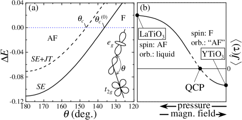
FIG. 3.: (a) Energy difference (in units of $J_{SE}^{(0)}$) between AF and ferromagnetic states as a function of $\theta$. The solid line is obtained within the SE model. Parameters are $\eta=0.12$ and $U/\Delta_{cr}=2.5$. The broken line includes small JT energy gain in the orbitally ordered ferromagnetic state. (b) Qualitative picture of the evolution of interactions in the spin channel. An average, static component of the spin exchange “constant” seen by coherent spin-waves is represented by a solid curve. Its sign depends on local correlations of orbitals. To the right of the critical point (QCP) these correlations are more antiferromagnetic, supported by noncollinear orbital orderings. To the left, the genuine ground state of the $t_{2g}$ system on cubic lattice, an orbital disordered state supporting spin AF, is stabilized. In the proximity area, a fluctuating part of the overall SE interaction dominates, and separation of the spin and orbital degrees of freedom might no longer be possible.

To conclude, the ferromagnetic phase of the $t_{2g}$ superexchange system has several competing orbital orderings with distinct physical properties. The elementary excitations of these states are identified. We find that Ti-O-Ti bond distortion favors the ferromagnetic state. Theory well explains recent neutron scattering results in YTiO₃. An orbital driven quantum phase transition in titanates remains a major challenge for future study.

We thank B. Keimer for stimulating discussions. Discussions with C. Ulrich, P. Horsch, R. Zeyher, S. Maekawa, J. Akimitsu, and S. Ishihara are acknowledged.

REFERENCES

- [1] Y. Tokura and N. Nagaosa, Science 288,462 (2000).
- [2] M. Imada, A. Fujimori, and Y. Tokura, Rev. Mod. Phys. 70, 1039 (1998).
- [3] J. B. Goodenough, Phys. Rev. 100, 564 (1955).
- [4] J. Kanamori, J. Phys. Chem. Solids 10, 87 (1959).
- [5] K. I. Kugel and D. I. Khomskii, Sov. Phys. Usp. 25, 231 (1982); Sov. Phys. Solid State 17, 285 (1975).
- [6] B. Keimer et al., Phys. Rev. Lett. 85, 3946 (2000).
- [7] G. Khaliullin and S. Maekawa, Phys. Rev. Lett. 85, 3950 (2000).
- [8] G. Khaliullin, Phys. Rev. B 64, 212405 (2001).
- [9] T. Katsufuji, Y. Taguchi, and Y. Tokura, Phys. Rev. B, 56, 10145 (1997).
- [10] C. Ulrich et al., preprint.
- [11] T. Mizokawa and A. Fujimori, Phys. Rev. B 54, 5368 (1996); H. Sawada and K. Terakura, Phys. Rev. B 58, 6831 (1998).
- [12] S. Ishihara, T. Hatakeyama, and S. Maekawa, Phys. Rev. B 65, 064442 (2002).
- [13] G. Khaliullin and S. Okamoto, (unpublished).
- [14] G. Khaliullin, P. Horsch, and A. M. Oleś, Phys. Rev. Lett. 86, 3879 (2001).
- [15] L. F. Feiner, A. M. Oleś, and J. Zaanen, Phys. Rev. Lett. 78, 2799 (1997).
- [16] G. Khaliullin and V. Oudovenko, Phys. Rev. B 56, R14 243 (1997).
- [17] R. P. Feynman, Statistical Mechanics (Benjamin, New York, 1972), Chap. 11.
- [18] H. Ichikawa et al., Physica B 281-282, 482 (2000).
- [19] The result of Ref. [7] corrected for the finite values of .