Unstable attractors induce perpetual synchronization and desynchronization

Abstract

Common experience suggests that attracting invariant sets in nonlinear dynamical systems are generally stable. Contrary to this intuition, we present a dynamical system, a network of pulse-coupled oscillators, in which unstable attractors arise naturally. From random initial conditions, groups of synchronized oscillators (clusters) are formed that send pulses alternately, resulting in a periodic dynamics of the network. Under the influence of arbitrarily weak noise, this synchronization is followed by a desynchronization of clusters, a phenomenon induced by attractors that are unstable. Perpetual synchronization and desynchronization lead to a switching among attractors. This is explained by the geometrical fact, that these unstable attractors are surrounded by basins of attraction of other attractors, whereas the full measure of their own basin is located remote from the attractor. Unstable attractors do not only exist in these systems, but moreover dominate the dynamics for large networks and a wide range of parameters.

As attractors determine the long-term behavior of dissipative dynamical systems, the notion of attractors is central to studies in many fields of science. According to the mathematical definitions of an attractor, states that originate in a certain volume of state space, the basin of attraction, evolve towards the respective attractor. Since states slightly perturbed from an attractor often stay confined to its vicinity and finally return to it, attractors are widely considered to be stable. Attracting yet unstable states are consistent with an attractor definition introduced by Milnor. There is evidence that such Milnor attractors might not be uncommon in certain systems that exhibit strange invariant sets with a fractal geometry. In general, however, unstable attractors seem to be special cases that have to be constructed artificially by precisely tuning parameters. Contrary to this intuition, we present an example of a dynamical system, a network of pulse-coupled oscillators, in which unstable attractors with periodic dynamics arise naturally. Unstable attractors are shown to prevail for large networks and a wide range of parameters. In the presence of arbitrarily weak noise, a perpetual synchronization and desynchronization of groups of oscillators occurs which leads to a switching among different attractors.

I Introduction

The concept of attractors is underlying the analysis of many natural systems as well as the design of artificial systems. For instance, the computational capabilities of neural networks are controlled by the attractors of their collective dynamics Hopfield ; Hertz ; Maass . Consequently, the nature and design of attractors in such systems constitute a focus of current research interest BressloffNC ; Diesmann ; ErnstPRE ; ErnstPRL ; GerstnerNC ; GerstnerPRL ; HanselPRL ; Mirollo ; Senn ; Timme ; Tsodyks ; vanVreeswijk . In general, the state space of a nonlinear dynamical system is partitioned into various basins of attraction from which states evolve towards the respective attractors. Since states that are slightly perturbed from an attractor often stay confined to its vicinity and eventually return to the attractor, attractors are commonly considered to be stable Eckmann ; Guckenheimer ; Katok .

In this paper we study the dynamics of networks of pulse-coupled oscillators ErnstPRE ; ErnstPRL ; Mirollo , in which unstable attractors exist and arise naturally as a collective phenomenon. Such models of pulse-coupled oscillators describe e.g. synchronization in spiking neural networks and the dynamics of other natural systems as diverse as pacemaker cells in the heart, populations of flashing fireflies, and earthquakes (cf. BressloffNC ; Buck ; Diesmann ; ErnstPRE ; ErnstPRL ; GerstnerNC ; GerstnerPRL ; HanselPRL ; Herz ; Mirollo ; Peskin ; Senn ; Strogatz ; Timme ; Tsodyks ; vanVreeswijk ). We identify an analytically tractable network exhibiting unstable attractors. For this network we demonstrate the existence of attractors that are unstable and located remote from the volume of their own basins of attraction. Such attracting yet unstable states are consistent with a definition of attractors introduced by Milnor, which neither presumes nor implies stability Milnor . In certain other systems such Milnor attractors might not be uncommon if these systems exhibit strange invariant sets with a fractal geometry Ashwin ; Kaneko ; Lai ; Sommerer ; Yang . More generally, however, attractors that are not stable seem to be special cases that have to be constructed artificially by precisely tuning parameters. Contrary to this intuition, in the system considered here, unstable attractors with regular, periodic dynamics are typical in large networks and persist even if the physical model parameters are varied substantially. The first discovery of the occurrence and prevalence of unstable attractors in networks of pulse-coupled oscillators was reported in Timme . Here we give a more detailed analysis of such unstable attractors and explain the observation that they only occur for excitatory (phase advancing) interactions but are absent if the interactions are inhibitory (phase retarding).

We argue that dynamical consequences of unstable attractors may persist in a general class of systems of pulse-coupled units. Such consequences include an ongoing switching among unstable attractors in the presence of noise. In systems where the convergence towards an attractor has a functional role, such as the solution of a computational task by a neural network Hertz ; Hopfield ; Maass , switching induces a high degree of flexibility that may provide the system with a unique advantage compared to multistable systems: In general, it is hard to leave a stable attractor after convergence, e.g. the completion of a task. With an unstable attractor, however, a small perturbation is sufficient to leave the attractor and to switch towards another one.

This paper is organized as follows: In section II we introduce a class of network models of pulse-coupled oscillators. We briefly review earlier results on synchronization phenomena in such networks within the framework introduced by Mirollo and Strogatz that is described in detail in section III. In section IV we describe the numerical observation that, in the presence of noise, trajectories approach and retreat from periodic orbits by perpetual synchronization and desynchronization of groups of oscillators. Together with further numerical investigations, this leads to the hypothesis, that the observed dynamics is induced by attractors that are unstable. In section V we perform an exact stability analysis of a particularly selected set of attractors. It is followed by an analysis of the dynamics during a switching transition between two states (Sec. VI) that is further corroborated by a numerical investigation of the structure of basins of attractions in state space. These results demonstrate that unstable attractors indeed exist in the class of networks of pulse-coupled oscillators considered. Section VII completes our analysis showing that unstable attractors prevail in large networks for a wide range of parameters. The paper concludes in section VIII with (i) a discussion of the dynamical consequence of switching among unstable attractors in comparison to smoothly coupled systems, (ii) a brief presentation of preliminary results for networks exhibiting different interactions or more complex structures and (iii) an outlook for future investigations.

II Models of pulse-coupled oscillators

In studies of synchronization phenomena in networks of pulse-coupled oscillators, single elements are often modelled as phase oscillators, assuming that the dynamics of the amplitude of the oscillation is less important. Thus there is only one relevant dynamical variable, $W_{i},$ that describes the dynamics of an individual oscillator $i$. In models of many natural systems, the oscillator variable $W_{i}$ represents an analogue of a potential, like the membrane potential in the case of a current-driven nerve cell. The dynamics of a network of pulse-coupled oscillators is commonly described by a system of coupled ordinary differential equations

$$\frac{dW_{i}}{dt} = A(W_{i})+B(W_{i})S_{i}(t)$$ (1)

for $i\in\{1,\ldots,N\}$ where $A$ and $B$ are continuous functions and $S_{i}$ represents the interactions within the network. The pulse-coupling between oscillators is given by

$$S_{i}(t)=\sum_{j=1}^{N}\sum_{m=-\infty}^{\infty}\varepsilon_{ij}K_{ij}(t-t_{j,m})$$ (2)

where $\varepsilon_{ij}$ is the strength of the coupling from oscillator $j$ to oscillator $i$ and the response kernels $K_{ij}(t)$ have the property that $K_{ij}(t)\geq 0$, $K_{ij}(t)=0$ for $t<0$, and $\int_{-\infty}^{\infty}K_{ij}(t)dt=1$. The sum includes all times $t_{j,m}$ at which oscillator $j$ reaches a threshold $W_{\theta}:=1$ (from below) for the $m^{\mathrm{th}}$ time,

$$W_{j}(t_{j,m})\geq W_{\theta}=1\,,\,\,\,\left.\frac{dW_{j}(t)}{dt}\right|_{t=t_{j,m}}>0.$$ (3)

If this threshold is reached, $W_{j}$ is reset to a potential

$$W_{j}(t_{j,m}^{+}):=W_{\mathrm{reset}}=0$$ (4)

and a signal is generated that is sent to oscillators $i$. Commonly, a unit that is reset and sends out a pulse when it reaches a threshold is said to “fire” at that instant of time. This form of pulse-coupling idealizes the fact that in diverse biological systems such as populations of flashing fireflies or networks of spiking neurons in the brain, units interact by stereotyped short-lasting signals that are generated as the state of a unit reaches a threshold. Note that the normalizations $W_{\theta}=1$ and $W_{\mathrm{reset}}=0$ are made without loss of generality. Whereas Eqs. (1)–(4) describe the interaction dynamics without delays between sending and reception of a pulse, a delay $\tau>0$ can easily be included by a transformation $K_{ij}(t)\rightarrow K_{ij}(t-\tau)$ of the response kernels.

It is often convenient vanVreeswijk (and under weak conditions possible) to transform the variables $W_{i}$ according to

$$V_{i}(t):=\frac{1}{C}\int_{0}^{W_{i}(t)}B(w)^{-1}dw$$ (5)

where

$$C=\int_{0}^{1}B(w)^{-1}dw$$ (6)

such that (1) becomes

$$\frac{dV_{i}}{dt} = \hat{A}(V_{i})+\frac{1}{C}S_{i}(t)$$ (7)

for $i\in\{1,\ldots,N\}$ where $\hat{A}(V)=C^{-1}A(W(V))/B(W(V))$ is determined solving Eq. (5) for $W$. If the duration of the response of a unit $i$ to an incoming pulse is sufficiently brief, the kernels $K_{ij}$ in (2) may be idealized by the Dirac distribution

$$K_{ij}(t)=\delta(t)$$ (8)

such that the coupling becomes discontinuous.

For the commonly used leaky integrate-and-fire models of oscillators the free dynamics is given by the linear inhomogeneous differential equation

$$\frac{dV}{dt}=-\gamma V+I$$ (9)

such that the network dynamics of such oscillators is given by substituting $\hat{A}(V_{i})=I-\gamma V_{i}$ in (7) where $I$ is an external current and $\gamma>0$ measures the dissipation in the system. This linear differential equation has the advantages that the solution is known explicitely and the response to an additional current can be found by superposition arguments. For sufficiently large external current, $I>\gamma$, the free ($S_{i}(t)\equiv 0$) dynamics

$$\left.\begin{array}[]{c}V(t)=I/\gamma\left(1-e^{-\gamma t}\right)\,\,\,\mathrm{for}\,\,0<t\leq T\\ V(t+T)=V(t)\end{array}\right.$$ (10)

is periodic (Fig. 1) with period $T=\frac{1}{\gamma}\ln\left(1-\frac{\gamma}{I}\right)^{-1}$.

Figure 1: Dynamics of a non-interacting integrate-and-fire oscillator. Without threshold, the potential $V$ would converge to its long-time limit $I/\gamma$ (dashed line). Every time the threshold $V_{\theta}=1$ is reached, the potential $V$ is reset to zero and a pulse is sent.

To study the synchronization of pacemaker cells in the heart, Peskin studied a simple, globally coupled network of such leaky integrate-and-fire oscillators Peskin where the coupling is not delayed, $\tau=0$, and the responses are infinitely fast, $K_{ij}(t)=\delta(t)$, excitatory, and homogeneous, $\varepsilon_{ij}=\varepsilon>0$. In his 1975 book he conjectured that arbitrary initial conditions converge towards the fully synchronous state in which all oscillators fire simultaneously. He gave a proof for $N=2$ oscillators assuming that both coupling strength and dissipation are small, $\varepsilon\ll 1$, $\gamma\ll 1$.

In a seminal work of 1990, Mirollo and Strogatz generalized the approach of Peskin Mirollo . Contrary to Peskin, whose analysis was based on the linearity of the differential equations, Mirollo and Strogatz’s only assumptions were that the free ($S_{i}(t)\equiv 0$) dynamics can be described by a phase-like variable and that the interactions are mediated by some potential function $U$ that is a monotonically increasing and concave down function of this phase Mirollo (for model details see below). This framework includes many cases for which the associated differential equation is nonlinear such that its solution may not be known explicitely and superposition arguments fail. Within this general framework, they proved that, for all $N$, almost all initial conditions will ultimately end up in the fully synchronous state. For systems without dissipation ($\gamma=0$), equivalent to linear functions $U$, Senn and Urbanczik Senn proved that the dynamics becomes fully synchronous even if the intrinsic frequencies and the thresholds of the oscillators are not quite identical. Like the previous investigators, they treated the case without delay, $\tau=0$, for which the fully synchronous state stays the only attractor. This periodic orbit is an example of period-one dynamics, for which every oscillator fires exactly once during one period, and is the simplest dynamics such a system may exhibit.

Within the framework introduced by Mirollo and Strogatz, it was, moreover, shown that the introduction of a delay time $\tau>0$, that occurs ubiquitously in natural systems, changes this situation drastically ErnstPRL ; ErnstPRE : With increasing network size, an exponentially increasing number of attractors coexist. In a large region of parameter space, these are periodic orbits with period-one dynamics, that exhibit several groups of synchronized oscillators (clusters), which reach threshold and send pulses alternately. It was also shown ErnstPRL ; ErnstPRE that these kinds of attractors arise not only in excitatorily coupled networks ($\varepsilon>0$) but also if the oscillators are coupled inhibitorily ($\varepsilon<0$).

In the following part of this paper, we show that for excitatory coupling, many of these periodic orbits with period-one dynamics are unstable attractors. As a consequence, trajectories converge towards these unstable attractors by synchronization of groups of oscillators into several clusters but, in the presence of arbitrarily weak noise, diverge subsequently via desynchronization of clusters.

III Mirollo-Strogatz model

We consider a homogeneous network of $N$ all-to-all pulse-coupled oscillators with delayed interactions. A phase-like variable $\phi_{i}(t)\in(-\infty,1]$ specifies the state of each oscillator $i$ at time $t$ such that the difference between the phases of two oscillators quantifies their degree of synchrony, with identical phases for completely synchronous oscillators. The free dynamics of oscillator $i$ is given by

$$d\phi_{i}/dt=1.$$ (11)

Whenever oscillator $i$ reaches a threshold

$$\phi_{i}(t)=1$$ (12)

the phase is reset to zero

$$\phi_{i}(t^{+})=0$$ (13)

and a pulse is sent to all other oscillators $j\neq i$, which receive this signal after a delay time $\tau$. The interactions are mediated by a function $U(\phi)$ specifying a ’potential’ of an oscillator at phase $\phi.$ The function $U$ is twice continuously differentiable, monotonically increasing, $U^{\prime}>0$, concave (down), $U^{\prime\prime}<0$, and normalized such that $U(0)=0$ and $U(1)=1$.

For a general $U(\phi)$ we define the transfer function

$$H_{\hat{\varepsilon}}(\phi)=U^{-1}(U(\phi)+\hat{\varepsilon})$$ (14)

that represents the response of an oscillator at phase $\phi$ to an incoming subthreshold pulse of strength $\hat{\varepsilon}$ that induces an immediate phase jump to $\phi^{+}=H_{\hat{\varepsilon}}(\phi)$. Depending on whether the input $\hat{\varepsilon}$ is subthreshold, $U(\phi)+\hat{\varepsilon}<1$, or suprathreshold, $U(\phi)+\hat{\varepsilon}\geq 1$, the pulse sent at time $t$ (Eq. (12)) induces a phase jump after a delay time $\tau$ at time $t^{\prime}=t+\tau$ according to

$$\phi_{j}({t^{\prime}}^{+})=\left\{\begin{array}[]{lll}H_{\hat{\varepsilon}}(\phi_{j}(t^{\prime}))&\mathrm{if}&U(\phi_{j}(t^{\prime}))+\hat{\varepsilon}<1\\ 0&\mathrm{if}&U(\phi_{j}(t^{\prime}))+\hat{\varepsilon}\geq 1\end{array}\right..$$ (15)

This phase jump (Fig. 2) depends on the phase $\phi_{j}(t+\tau)$ of the receiving oscillator at a time $\tau$ after the signal by oscillator $i$ has been sent at time $t$, the effective coupling strength $\varepsilon_{ij}=\hat{\varepsilon}=\varepsilon/(N-1)$, and the nonlinear potential $U$.

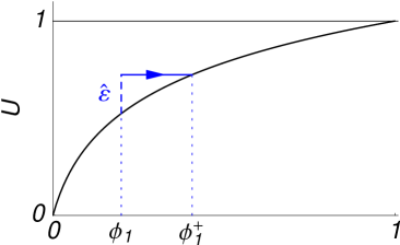
Figure 2: An incoming pulse of strength $\hat{\varepsilon}$ induces a phase jump $\phi_{1}^{+}:=\phi_{1}(t^{+})=U^{-1}(U(\phi_{1}(t))+\hat{\varepsilon})=H_{\hat{\varepsilon}}(\phi_{1})$ that depends on the state $\phi_{1}:=\phi_{1}(t)$ of the oscillator at time $t$ of pulse reception. Due to the monotonicity of $U$, an excitatory pulse ($\hat{\varepsilon}>0$) induces an advancing phase jump. If the incoming pulse puts the potential above threshold ($U(\phi_{1})+\hat{\varepsilon}>1$), the phase is reset to zero ($\phi_{1}^{+}=0$). An inhibitory pulse ($\hat{\varepsilon}<0$) would induce a regressing phase jump such that the phase may assume negative values (not shown).

The interactions are either excitatory ($\varepsilon>0$) inducing advancing phase jumps (Fig. 2) or inhibitory ($\varepsilon<0$) inducing retarding phase jumps. Note that in response to the reception of an inhibitory pulse, the phases of the oscillators may also assume negative values.

The general class of functions $U$ captures the dynamics of a variety of systems. In particular, given any differential equation of the form (7) the free ($S_{i}(t)\equiv 0$) dynamics of which has a monotonic periodic solution $V(t)$ with period $T$ and negative curvature, the function $U$ can be taken as the scaled solution,

$$U(\phi):=V(\phi T).$$ (16)

By this transformation, the general class of pulse-coupled oscillators (Eqs. (1)–(4)) with infinitely fast response (8) is mapped onto a normalized phase description (Eqs. (11)–(15)). For instance, the standard leaky integrate-and-fire oscillator (9) with solution (10) leads to

$$U_{\mathrm{IF}}(\phi)=\frac{I}{\gamma}(1-e^{-\gamma\phi T})=\frac{I}{\gamma}\left(1-\left(1-\frac{\gamma}{I}\right)^{\phi}\right).$$ (17)

Another example is given by the conductance-based threshold model of a neuron Johnston , in which $A(W)=\gamma(W_{\mathrm{eq}}-W)$ and $B(W)=g(W_{\mathrm{s}}-W)$ with equilibrium potential $W_{\mathrm{eq}}>1$, membrane time constant $\gamma>0$, synaptic reversal potential $W_{\mathrm{s}}$, and conductivity $g>0$. After a transformation of variables $V=V(W)$ according to (5) and a scaling (16) we obtain

$$U_{\mathrm{CB}}(\phi)=\frac{\ln\left(1+W_{\mathrm{eq}}/W_{\mathrm{s}}\left[\left(1-W_{\mathrm{eq}}^{-1}\right)^{\phi}-1\right]\right)}{\ln\left(1-W_{\mathrm{s}}^{-1}\right)}.$$ (18)

The resulting potential function $U$ is always monotonically increasing and, for a wide range of biologically reasonable values of $W_{\mathrm{s}}$ and $W_{\mathrm{eq}}$, also concave down.

For all numerical studies and simulations presented in this paper, we use the functional form

$$U(\phi)=U_{b}(\phi)=b^{-1}\ln\left(1+(e^{b}-1)\phi\right)$$ (19)

that results in an affine transfer function $H_{\hat{\varepsilon}}(\phi)=e^{\hat{\varepsilon}b}\phi+\mathrm{const}$, that was utilized also in the original work of Mirollo and Strogatz Mirollo as well as in the later investigation of the influence of delay ErnstPRL ; ErnstPRE .

Compared to systems of nonlinear differential equations, the Mirollo-Strogatz approach has the additional advantage, that numerical calculations can be performed exactly on an event-by-event basis. Given the state of the system at time $t$, defined by a phase vector $\boldsymbol{\phi}(t)$ and a list of signals sent together with their sending times, the dynamics can be computed numerically by iterating between two kinds of events (in an appropriate order):

1. If the next event is the reception of a signal after a time $\Delta t_{1}$, shift all phases $\phi_{i}(t)$ by this amount and apply the map $H_{\hat{\varepsilon}}$ according to Eq. (15). If the received signal is subthreshold for oscillator $j$, its resulting phase is given by

   $$\phi_{j}(t+\Delta t_{1})=H_{\hat{\varepsilon}}(\phi_{j}(t)+\Delta t_{1})\,,$$ (20)

   if the signal is suprathreshold for oscillator $j^{\prime}$,  $\phi_{j^{\prime}}(t)+\Delta t_{1}\geq 1$, its phase is reset to zero,

   $$\phi_{j^{\prime}}(t+\Delta t_{1})=0.0\,,$$ (21)

   and a signal is generated, i.e. its sending time $t+\Delta t_{1}$ and the set of sending oscillators $j^{\prime}$ is stored. If $k>1$ signals have been simultaneously sent by synchronized oscillators their simultaneous arrival can simply be numerically realized by an enlarged coupling strength $(k-1)\hat{\varepsilon}$ or $k\hat{\varepsilon}$, depending on whether or not the considered receiving oscillator has sent one of the $k$ signals.

2. If the next event is that one or more oscillators reach threshold after time $\Delta t_{2}=1-\max_{i}\phi_{i}(t)$ (without receiving an additional input signal after a time $\Delta t_{1}<\Delta t_{2}$), those oscillators $j$ are reset to zero,

   $$\phi_{j}(t+\Delta t_{2})=0.0\,,$$ (22)

   and a signal is generated (see event 1.) whereas the phases of all other oscillators $j^{\prime}$ are just translated in time according to

   $$\phi_{j^{\prime}}(t+\Delta t_{2})=\phi_{j^{\prime}}(t)+\Delta t_{2}\,.$$ (23)

These are the only two possible events that change the state of the system, such that the simulation time is increased by $\Delta t_{1}$ or $\Delta t_{2}$, depending on the kind of event: To determine the state at the next time step after time $t$ numerically, one first finds the minimum of the time $\Delta t_{1}$ after which the next signal would arrive and the time $\Delta t_{2}$ after which the next phase would cross threshold without an additional incoming signal (cf. Eq. (15)). Thus, time steps smaller than $\Delta t_{\mathrm{MS}}=\min\{\Delta t_{1}\,,\Delta t_{2}\}$ do not need to be considered. Note that $\Delta t_{\mathrm{MS}}$ depends on the state of the system such that it changes with time $t$.

This event-based numerics can be exploited for every choice of $U(\phi)$, and is not restricted to $U_{\mathrm{IF}}(\phi)$ derived from the linear differential equation (9), for which one may as well exactly numerically integrate the original differential equation due to linear superposition (cf. Rotter ; Hansel_Num ).

Hence, in contrast to standard numerical integration of nonlinear differential equations, for which the time steps $\Delta t_{\mathrm{DE}}$ have to be taken sufficiently small and the numerics is only approximate, the above numerical algorithm for the Mirollo-Strogatz model is exact. It is also fast, if oscillators constitute synchronized groups, because then typical time steps are long, $\Delta t_{\mathrm{MS}}\gg\Delta t_{\mathrm{DE}}$.

IV Perpetual synchronization and Desynchronization

For such pulse-coupled systems, periodic orbits with groups of synchronized units constitute relevant attractors BressloffNC ; Buck ; Diesmann ; ErnstPRE ; ErnstPRL ; GerstnerNC ; GerstnerPRL ; Herz ; Mirollo ; Peskin ; Senn ; Strogatz ; Tsodyks ; vanVreeswijk . As mentioned above, for the networks of Mirollo-Strogatz oscillators with delayed interactions ($\tau>0$) considered here, many different cluster-state attractors with several synchronized groups of oscillators (clusters) coexist ErnstPRE ; ErnstPRL . After an initial transient, these networks settle down onto such a periodic orbit that displays period-one dynamics with clusters firing successively within each period. Thus, in particular, phase-differences between oscillators are constant at all times when a reference oscillator is reset.

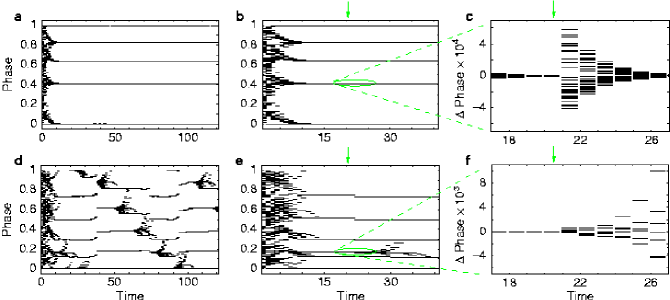
Figure 3: Phase dynamics of a large network ($N=100$, $\tau=0.15$). Phases of all oscillators are plotted whenever a reference oscillator has been reset such that the axis labeled ’Time’ is discrete and nonlinear. (a,b,c) Inhibitory coupling ($\varepsilon=-0.2$). (d,e,f) Excitatory coupling ($\varepsilon=0.2$). (a,d) Dynamics with noise (noise level $\eta=10^{-3}$). (b,e) Deterministic dynamics in response to a single phase perturbation (arrow, perturbation strength $\sigma=10^{-3}$); (b) for inhibitory coupling the system returns to the attractor; (e) for excitatory coupling the system switches from a six-cluster to a five-cluster state. (c,f) Phase differences from the average phase of one cluster (shown in b and e, respectively) in response to the perturbation.

Whereas the noise-free dynamics is seemingly similar for both kinds of coupling, in the presence of noise the collective behavior of excitatorily coupled oscillators strongly differs from that of oscillators coupled inhibitorily. For inhibitory coupling all cluster-state attractors are stable against small perturbations. Under the influence of sufficiently weak noise the system stays near some periodic orbit that has been reached after a transient from a random initial state (Fig. 3a). The dynamics after a small perturbation in an otherwise noiseless system confirms this stability property: Perturbations to all clusters decay exponentially and the original attractor is approached again (Fig. 3b,c).

In contradistinction, for excitatory coupling, we find (cf. Fig. 3d) that, although the system converges towards a periodic orbit from random initial states, small noise is often sufficient to drive the system away from that attractor such that successive switching towards different attractors occurs. In principle, this dynamics might be due to stable attractors located close to the boundaries of their basins of attraction, such that noise drives the trajectory into a neighboring basin. If this explanation were correct, ever smaller perturbations off the attractor would lead to an ever lower probability of leaving its basin. In an otherwise noiseless system we tested this possibility by applying instantaneous, uniformly distributed, independent random perturbations $\delta_{i}\in[0,\sigma]$ of gradually decreasing strengths (down to $\sigma=10^{-14}$) to the phases $\phi_{i}$ of all oscillators $i$ after the system had settled down to an attractor (see Fig. 3e,f). Even for the weakest perturbations applied, none of the perturbed states returned to the attractor, but all trajectories separated from the original attractor. We thus hypothesized that the persistent switching dynamics (Fig. 3d) is due to attractors that are unstable.

V Stability analysis

In order to verify this hypothesis directly, we analyze a small network of $N=6$ excitatorily coupled oscillators for which instantaneous perturbations lead to a similar switching among attractors. We fix parameters to $\varepsilon=0.2$, $\tau=0.15$ and the potential function $U(\phi)=U_{3}(\phi)$ according to Eq. (19). At these parameters the network exhibits a set of periodic orbits with period-one dynamics that are related by a permutation of phases in such a way, that the system may switch among them (cf. Fig. 4a, points on the periodic orbits marked in red, yellow, blue). These orbits are structurally stable in a neighborhood of these parameters and the function $U$. Each attractor can be characterized by a list of cluster occupation numbers giving the number of oscillators $n_{k}$ in the $k^{\mathrm{th}}$ cluster, counted in the order of increasing phases at times after a reference oscillator ($i=1$) has been reset. For instance, the attractor marked in yellow is characterized by the occupation list $[2,2,1,1]$ such that the transitions among the attractors (Fig. 4a) are described by the sequence ($[1,2,2,1]$ (red) $\rightarrow$ $[2,2,1,1]$ (yellow) $\rightarrow$ $[2,1,1,2]$ (blue) $\rightarrow$ $[1,2,2,1]$ (red)) for the particular set of perturbations applied. For each of these three attractors there exists another permutation-related attractor with the same occupation list but with the phase values of the two clusters containing only one oscillator interchanged. It turns out that, depending on the perturbation, transitions from one attractor occur to one of only two other attractors that are related through the latter permutation. Thus, once the system has settled down to one of the attractors shown, it may switch within a set of six periodic orbit attractors in response to sufficiently small perturbations.

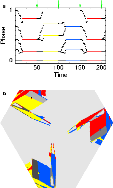
Figure 4: Small network ($N=6$, $\varepsilon=0.2$, $\tau=0.15$) exhibiting unstable attractors. (a) Noise-free phase dynamics in response to instantaneous perturbations of magnitude $\sigma=10^{-3}$ (arrows). When an attractor is reached, the phase configuration specifying the current cluster state attractor is marked in color. The perturbations induce a split-up of clusters and a divergence from the attractor such that the network reaches different attractors successively. For the realization of perturbations shown, the attractors marked in red (cluster occupation list $[1,2,2,1]$), yellow ($[2,2,1,1]$), and blue ($[2,1,1,2]$) are visited cyclically. For each of the three attractors there exists another attractor with the same cluster occupation list but with phase values of the two clusters with only one oscillator interchanged. (b) Basin structure of the three attractors color-marked in (a) in two-dimensional planar section through six-dimensional state space. The planar section is defined by one point on each of the three periodic orbit attractors, represented by small red, yellow, and blue disks, respectively. Basins of the three attractors are marked in the same colors. The part of state space within this section is of hexagonal shape. Darker gray areas are basins of the three other permutation-related attractors (cf. (a)) that are located outside the section shown. Lightest gray marks the union of the basins of all other attractors.

Due to their permutation-equivalence these orbits have identical stability properties. The state of the network at time $t$ is specified by $\boldsymbol{\phi}(t)=(\phi_{1}(t),\ldots,\phi_{6}(t))^{\mathsf{T}}$, such that the orbit marked in yellow in Fig. 4a is defined by the initial condition

$$\boldsymbol{\phi}(0)=(0,\,0,\,A,\,A,\,B,\,C)^{\mathsf{T}}$$ (24)

where

$$A = H_{\hat{\varepsilon}}(\tau)$$ (25)

$$B = H_{2\hat{\varepsilon}}(1+2\tau-a_{4})$$ (26)

$$C = H_{2\hat{\varepsilon}}(H_{\hat{\varepsilon}}(2\tau)+1+\tau-a_{4})$$ (27)

and recursively defined

$$a_{i}=U^{-1}(k_{i}\hat{\varepsilon}+U(\tau+a_{i-1}))$$ (28)

for $i\in\{1,\ldots,4\}$, $a_{0}=0$, and $k_{1}=k_{3}=k_{4}=1$, $k_{2}=2$. Here the origin of time, $t=0$, was chosen such that oscillators $1$ and $2$ have just sent a signal and have been reset. Moreover, at $t=0$ only these two signals (and no others) have been sent but not yet received. The numerical values for the particular parameters considered, $A\approx 0.176$, $B\approx 0.499,$ $C\approx 0.747$, can be identified in Fig. 4a (orbit marked in yellow). This orbit indeed is periodic,

$$\boldsymbol{\phi}(T)=\boldsymbol{\phi}(0),$$ (29)

and, in particular, period-one, such that each oscillator fires exactly once during one period $T$.

To perform a stability analysis, we define a Poincare map by choosing oscillator $i=1$ as a reference: Let

$$\phi_{n,i}:=\phi_{i}(t_{n}^{+})$$ (30)

be the perturbed phases of the oscillators $i$ at times $t_{n}>0$, $n\in\mathbb{N}$, just after the resets of oscillator $1$,

$$\phi_{1}(t_{n}^{+})\equiv 0.$$ (31)

Thus the five-dimensional vector

$$\boldsymbol{\delta_{n}}=\boldsymbol{\phi_{n}}-(0,\,A,\,A,\,B,\,C^{\prime})^{\mathsf{T}}$$ (32)

defines the perturbations $\delta_{n,i}$ for $i\in\{2,\ldots,6\}$ where we choose $0<\delta_{n,2}$ and $\delta_{n,3}<\delta_{n,4}$. Here

$$C^{\prime}=H_{2\hat{\varepsilon}}(H_{\hat{\varepsilon}}(2\tau+H_{\hat{\varepsilon}}(0))+1+\tau-a_{4})$$ (33)

that numerically yields $C^{\prime}\approx 0.756.$ Because after a general perturbation clusters are split up such that in particular $\phi_{1}<\phi_{2}$, oscillator $6$ receives the (later) signal from oscillator $1$ only after it is reset by the (earlier) signal from oscillator $2$ resulting in $C^{\prime}\neq C$. Thus, the original orbit is super-unstable, i.e. has infinite expansion rate and the stability analysis is performed for the orbit obtained in the limit $\boldsymbol{\delta}_{n}\rightarrow\mathbf{0}$. It is important to note that unstable attractors also exist that do not posses such a “partner orbit” but have a finite expansion rate themselves. For convenience, we here continue considering the above set of orbits that allow a straightforward explanation of the phenomenon of unstable attraction. Following the dynamics, the five-dimensional Poincare map is given by

$$\boldsymbol{\delta}_{n+1}=\boldsymbol{F}(\boldsymbol{\delta}_{n}),$$ (34)

where $\boldsymbol{F}$ is defined by

$$\left.\begin{array}[]{lll}F_{2}(\boldsymbol{\delta})&=&0\\ F_{3}(\boldsymbol{\delta})&=&L_{4}-L_{3}+H_{\hat{\varepsilon}}(\tau-L_{4}+L_{3})-A\\ F_{4}(\boldsymbol{\delta})&=&H_{\hat{\varepsilon}}(\tau+L_{4}-L_{3})-A\\ F_{5}(\boldsymbol{\delta})&=&H_{\hat{\varepsilon}}(H_{\hat{\varepsilon}}(1+2\tau-L_{4})+L_{4}-L_{3})-B\\ F_{6}(\boldsymbol{\delta})&=&H_{\hat{\varepsilon}}(L_{4}-L_{3}+H_{\hat{\varepsilon}}(\tau+1-L_{3}+\\ &&\,\,\,H_{\hat{\varepsilon}}(2\tau-\delta_{2}+H_{\hat{\varepsilon}}(\delta_{2}))))-C^{\prime}\end{array}\right.$$ (35)

with the abbreviations

$$\left.\begin{array}[]{ccc}L_{i}:=L_{i}(\boldsymbol{\delta})&=&H_{\hat{\varepsilon}}(\tau+H_{\hat{\varepsilon}}(\tau-\delta_{2}+H_{\hat{\varepsilon}}(\delta_{2}+\\ &&\,\,\,H_{\hat{\varepsilon}}(\tau+\delta_{i}-\delta_{2}+H_{\hat{\varepsilon}}(\tau)))))\end{array}\right.$$ (36)

for $i\in\{3,4\}$. Here the difference $L_{4}-L_{3}$ in Eqs. (35) is of order $L_{4}-L_{3}=\mathcal{O}(\left\|\boldsymbol{\delta}\right\|)$.

The linearized dynamics

$$\boldsymbol{\delta}_{n+1}\doteq M\boldsymbol{\delta}_{n}$$ (37)

of a slightly perturbed state with split-up clusters is described by the Jacobian matrix

$$M=\left.\frac{\partial\boldsymbol{F}(\boldsymbol{\delta})}{\partial\boldsymbol{\delta}}\right|_{\boldsymbol{\delta}=\mathbf{0}}=\left(\begin{array}[]{ccccc}0&0&0&0&0\\ 0&\alpha&-\alpha&0&0\\ 0&-\beta&\beta&0&0\\ &*&*&0&0\\ &*&*&0&0\end{array}\right)$$ (38)

where $\alpha,\beta>0$ and $*$ denote nonzero real numbers. It has four zero eigenvalues

$$\lambda_{i}=0\,\,\,\mathrm{for}\,\,\,i\in\{1,2,3,4\}$$ (39)

which imply that a six-dimensional state-space accessed by the random perturbation is contracted onto a two-dimensional manifold. This reflects the fact that suprathreshold input received simultaneously by two or more oscillators (Fig. 5) leads to a simultaneous reset and thus a synchronization of these oscillators independent of their precise phases. If a single oscillator is reset by a suprathreshold signal, it instantaneously exhibits a precise lag in firing time $\Delta t=\tau$ compared to the oscillator that has sent this signal.

In particular, the zero eigenvalues (Eq. (39)) reflect the following contracting dynamics: (i) Perturbations of phases $\delta_{n,5}\neq 0$ or $\delta_{n,6}\neq 0$ are restored immediately by suprathreshold input pulses received from oscillators $j=6$ or $j=1$, respectively. This gives rise to the eigenvalues $\lambda_{1}=\lambda_{2}=0$ corresponding to the eigenvectors $v_{1}\propto(0,0,0,1,0)^{\mathsf{T}}$ and $v_{2}\propto(0,0,0,0,1)^{\mathsf{T}}$. (ii) A splitting of the first cluster, $\delta_{n,2}>0\equiv\delta_{n,1}\,$, corresponding to the vector $v_{3}\propto(1,0,0,0,0)^{\mathsf{T}}$, is restored after one period due to one suprathreshold input pulse from oscillator $j=4$. At the same time, however, this splitting induces a perturbation of oscillators $i=5$ and $i=6$ such that $\delta_{n+1,5}\neq 0$ and $\delta_{n+1,6}\neq 0$ which is restored according to (i) in the subsequent period. Taken together, this accounts for the eigenvalue $\lambda_{3}=0$. (iii) As long as $\delta_{n,3}=\delta_{n,4}\,$, a perturbation vector is mapped onto the subspace spanned by $v_{1}$ and $v_{2}$ (see (i)) within one period and is then mapped onto zero during the next period. As a result, the eigenvalue $\lambda_{4}=0$ corresponds to the direction $v_{4}\propto(0,1,1,0,0)^{\mathsf{T}}$. In addition to this analysis, a stability analysis for the subset of states with the cluster $\phi_{3}(t)\equiv\phi_{4}(t)$ kept synchronized, results in superstable directions only, as expected.

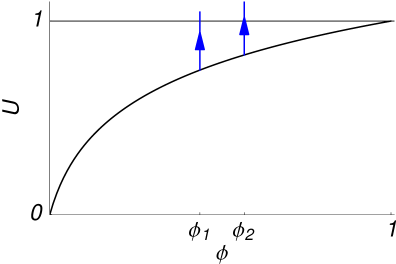
Figure 5: Simultaneous suprathreshold excitatory input synchronizes immediately due to the reset at threshold. Sufficiently small but positive phase differences $\left|\phi_{2}(t)-\phi_{1}(t)\right|>0$ are reduced to zero such that $\phi_{2}(t^{+})=\phi_{1}(t^{+})=0$. This is the mechanism of dimensional reduction of effective state space, by which attractors can be built.

In contradistinction to this contracting dynamics, the concavity of $U$ implies that simultaneous subthreshold input to two or more oscillators leads to an increase of their phase differences, i.e. a desynchronization of oscillators with similar phases (Fig. 6).

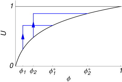
Figure 6: Simultaneous subthreshold excitatory input desynchronizes due to the concavity of $U$. Small phase differences $\left|\phi_{2}(t)-\phi_{1}(t)\right|>0$ are increased, $\left|\phi_{2}(t^{+})-\phi_{1}(t^{+})\right|>\left|\phi_{2}(t)-\phi_{1}(t)\right|$, providing the mechanism that creates an instability.

For the orbits considered here, this is reflected by the only non-zero eigenvalue

$$\lambda_{5}=\frac{(2U^{\prime}(c_{0})-U^{\prime}(a_{1}))U^{\prime}(c_{1})U^{\prime}(c_{2})U^{\prime}(c_{3})}{U^{\prime}(a_{1})U^{\prime}(a_{2})U^{\prime}(a_{3})U^{\prime}(a_{4})}>1$$ (40)

where

$$c_{i}=\tau+a_{i}$$ (41)

for $i\in\{0,1,2,3\}$ and the $a_{i}$ are defined in Eq. (28). Because $c_{i}>a_{i}>c_{i-1}$ for all $i$ and $U^{\prime}>0$, $U^{\prime\prime}<0$, this eigenvalue is larger than one, i.e. the periodic orbit is linearly unstable. This eigenvalue corresponds to a split-up of the cluster composed of the oscillators $i=3$ and $i=4$. Because the Jacobian (38) is not symmetric, the eigenvectors are not orthogonal such that the corresponding eigenvector is not $v\propto(0,1,-1,0,0)^{\mathsf{T}}$ but has a component in this direction. If there is no homoclinic connection, this instability implies that such an attractor is not surrounded by a positive volume of its own basin of attraction, but is located at a distance from it: Thus, every random perturbation to such an attractor state – no matter how small – leads to a switching towards a different attractor.

VI Unstable Attractors

Furthermore, this periodic orbit indeed is an attractor: According to the stability analysis, after two firings of the reference oscillator, a trajectory perturbed off a periodic orbit (e.g. the one marked in red in Fig. 4a, which is permutation-equivalent to the yellow one) is mapped onto a two-dimensional manifold, re-synchronizing one cluster. The trajectory then evolves towards a neighborhood of another attractor (here: the yellow one) in a lower dimensional effective state space without further dimensional reduction. Here, forming the second cluster, suprathreshold input leads to the last dimensional reduction while the state is mapped directly onto the periodic orbit.

In general, a periodic orbit is unstable if, after a random perturbation into its vicinity, one or more clusters are not re-synchronized by simultaneous suprathreshold input but desynchronize due to simultaneous subthreshold input. An unstable attractor results if these clusters are formed through synchronization in a region of state space that is located remote from the periodic orbit towards which the state then converges.

Although this is a discontinuous system with delayed interactions such that there is no simple basin structure in the state space of phases and signals, a three-dimensional cartoon of the basin structure in a state space of phases may help to gain further insight about how trajectories approach and retreat from an unstable attractor in the presence of noise.

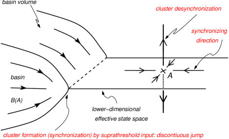
Figure 7: Cartoon of the basin structure of an unstable attractor $A$. First, a positive basin volume $B(A)$ of states is mapped onto a lower-dimensional effective state space. This is achieved by simultaneous suprathreshold input to a group of oscillators, that synchronizes them to form one cluster. Because the attractor is located remote from its own basin volume the same cluster may desynchronize in response to small perturbations near the attractor, where incoming pulses are no longer supra- but subthreshold and thus lead to a desynchronization.

Figure 7 shows that the basin volume is contracted by creating (at least) one cluster in a region of state space that is remote from the attractor itself. In contrast, near the attractor, the same cluster is unstable against a split-up of the phases of the oscillators it contains. Basically, such an unstable attractor might be viewed as an unstable periodic orbit with a remote basin attached to its stable manifold that ensures the attractivity property.

It is important to note that for inhibitory coupling we observe that all attractors are stable: An intuitive explanation is that there is only a mechanism of synchronization (Fig. 8) due to the concavity of $U$ that contracts state space volume such that all attractors with period-one dynamics are stable. It is instructive to compare Fig. 8 for inhibition to Fig. 6 for excitation that display how simultaneously incoming subthreshold pulses affect phase differences.

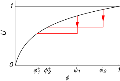
Figure 8: Simultaneous inhibitory input synchronizes due to the concavity of $U$. Contrary to networks of oscillators coupled excitatorily, here the inhibitory interactions allow subthreshold input only and lead to a decrease of phase differences, $\left|\phi_{2}(t^{+})-\phi_{1}(t^{+})\right|>\left|\phi_{2}(t)-\phi_{1}(t)\right|$ . Hence, these networks possess a mechanism for synchronization, but there is no simple possibility of desynchronizing a cluster state.

Since for inhibition all attractors are period-one states ErnstPRE ; ErnstPRL , we expect that the possibility of unstable attractors is excluded for this kind of coupling.

In order to further clarify the structure of state space of networks of excitatorily coupled oscillators, we numerically determined the basins of attraction of the three attractors displayed in Fig. 4a in two-dimensional sections of state space. The example shown in Fig. 4b reveals that attractors are surrounded by basins of attraction of other attractors as predicted by the above analysis. Because of this basin structure, noise induces repeated attractor switching among unstable attractors. Starting from the orbit defined by (24) the system may switch within sets of only six periodic orbit attractors as is apparent from the basins shown in Fig. 4b. However, in larger networks (cf. e.g. Fig. 3d) a cluster may split up in a combinatorial number of ways and exponentially many periodic orbit attractors are present among which the system may switch. The larger such networks are, the higher the flexibility they exhibit in visiting different attractors and exploring state space.

Until now, the analysis has focussed on a small network of $N=6$ oscillators, for which certain periodic orbits have been demonstrated to be unstable attractors. To study the desynchronization of clusters also observed in larger network in greater detail, we numerically determined the divergence of small random perturbations to an attractor in a network of $N=100$ oscillators. As an example we chose two perturbations $\boldsymbol{\delta_{1}}=\sigma_{1}\boldsymbol{\delta^{*}}$ and $\boldsymbol{\delta_{2}}=\sigma_{2}\boldsymbol{\delta^{*}}$ into the same random direction $\boldsymbol{\delta^{*}}\in[0,1]^{N}$ where $\sigma_{1}=10^{-12}$ and $\sigma_{2}=\sigma_{1}+10^{-14}$. Figure 9 shows that the separation $\Delta:=\max_{i}|\delta_{1,i}-\delta_{2,i}|$ between the two perturbed trajectories exponentially increases with time. This indicates that also for large networks, desynchronization is due to a linear instability. Let us remark that, due to the spiltting-up of clusters by a general perturbation (cf. Eqs. (32) and (33)), two perturbations into independent directions might first lead to an additional discontinuous separation, followed by an exponential expansion.

Figure 9: Separation of two perturbations off an unstable attractor into the same random direction for a large network ($N=100$, $\varepsilon=0.2$, $\tau=0.15$). The separation $\Delta$ grows exponentially with the time after the perturbation, measured in number of firing events of a reference oscillator.

As a second quantity, that characterizes the dynamics of switching, we consider the time needed by the system to switch from an unstable attractor towards a different attractor after a random perturbation of magnitude $\sigma$. The perturbations applied to the attractor are random phase vectors, drawn from a uniform distribution on $[0,\,\sigma]^{N}$, with $\sigma\in[10^{-12},10^{-2}]$. As displayed in Fig. 10, for sufficiently small $\sigma$, this switching time clearly increases exponentially with decreasing $\sigma$. In particular, this indicates that the attractors found are indeed unstable and do not possess small contracting open neighborhoods. Furthermore, it confirms our observations that the time of switching is mainly determined by the time of divergence from the original unstable attractor. Thus, in the presence of external noise, we expect a similar monotonic increase of an approximate switching time with the amplitude of the noise.

Figure 10: Time of switching between two attractors depending on the perturbation strength $\sigma$ for a large network ($N=100$, $\varepsilon=0.2$, $\tau=0.15$). The switching time increases exponentially with decreasing perturbation strength. The discrete time axis (number of firing events of a reference oscillator) leads to a regular stepping that slightly disrupts the exponential trend.

Taken together, this indicates that there exist also unstable attractors in larger networks that are enclosed by basins of other attractors. Thus, these results strongly support the hypothesis, that the switching found in large networks in the presence of noise (cf. Fig. 3), is also due to unstable attractors. It is important to note that, without a perturbation, numerical noise does not induce a divergence of trajectories from attractors which are unstable: Synchronization occurs by simultaneously resetting the phases of two or more oscillators to zero (cf. Fig. 5). Due to the global homogeneous coupling, all signals simultaneously received by these oscillators are of the same size and are exactly synchronous numerically (see Sec. III). Thus, although the phase-advance computed for such signals is influenced by numerical round-off errors, such errors will be identical for phases of synchronized oscillators and hence not induce a numerical desynchronization.

VII Prevalence and persistence

The preceeding analysis demonstrates the existence of unstable attractors. For excitatory coupling, these unstable attractors coexist with stable attractors. For a cluster-state attractor to be stable, all clusters necessarily receive suprathreshold input once per period that re-synchronizes possibly split-up oscillators. In general, a stable attractor has a contracting neighborhood in state space from which perturbed trajectories return to the attractor. If an attractor is unstable there are trajectories arbitrarily close to the attractor, which diverge from it, such that unstable attractors do not exhibit a contracting neighborhood. In other words, an unstable attractor has to be located at the boundary of its own basin. Therefore, the intuitive expectation is that parameters of the system have to be precisely specified in order to keep a periodic orbit simultaneously attracting and unstable. This leads to the question whether the physical parameters of the system, in particular $\varepsilon$, $\tau$, and $N$, need to be precisely tuned to obtain unstable attractors.

To answer the question, how common unstable attractors actually are, we numerically estimated the fraction $p_{\mathrm{u}}(N)$ of state space occupied by basins of unstable attractors. To obtain this estimate, we initialized the system with 1000 random initial phase vectors, drawn from the uniform distribution on $[0,1]^{N}$. Whenever a period-one orbit was reached, we applied one random phase perturbation $\boldsymbol{\delta}$ drawn from the uniform distribution on $[0,\sigma]^{N}$where we chose $\sigma=10^{-6}$, a value well below all scales that are determined by the model parameters, in particular $\sigma\ll\varepsilon/N$ for network sizes up to $N\approx 10^{2}$. If perturbed trajectories did not return to the original attractor, it was counted unstable. If no period-one orbit was reached from a random initial state but, e.g., orbits of higher period, these were not tested for stability. Thus, the numerical method used estimates a lower bound on $p_{\mathrm{u}}(N)$. As an example, Fig. 11a displays such an estimate of $p_{\mathrm{u}}(N)$ for $\varepsilon=0.2$ and $\tau=0.15$.

Figure 11: Prevalence of unstable attractors in large networks. (a) Unstable attractors prevail for large networks for certain parameters ($\varepsilon=0.2$, $\tau=0.15)$, but (b) are not important in large networks for other parameters ($\varepsilon=0.2$, $\tau=0.25$). The fraction $p_{\mathrm{u}}(N)$ was estimated for every $N\leq 128$ from $1000$ random initial phase vectors, drawn from the uniform distribution on $[0,1]^{N}$.

Figure 12: Unstable attractors persist in a wide region of parameter space in large networks ($N=100$). Parameters with $p_{\mathrm{u}}(100)>0.5$ are marked in black; here $p_{\mathrm{u}}(100)$ was estimated from $100$ random initial phase vectors, drawn from the uniform distribution on $[0,1]^{N}$, for every set of parameters (resolution $\Delta\tau=\Delta\varepsilon=0.005$).

While for these parameters unstable attractors are absent if networks are too small (here $N\leq 4$) and coexist with stable attractors in larger networks, the fraction approaches one for $N\gg 1$. Other parameters ($\varepsilon=0.2$, $\tau=0.25$) yield a different dependence on the network size $N$. Once again, unstable attractors arise only if the network size is not too small ($N\geq 3)$. Yet, the fraction $p_{\mathrm{u}}(N)$ is only substantial for moderate network sizes near $N\approx 10$ and approaches zero for large $N$. More generally, we observed that unstable attractors are absent in small networks (cf. ErnstPRE ; ErnstPRL for the case $N=2$) and $p_{\mathrm{u}}(N)$ approaches either zero or one in large networks, depending on the parameters. For networks of $N=100$ oscillators, Fig. 12 shows the region of parameter space in which unstable attractors prevail ($p_{\mathrm{u}}(100)>0.5$, estimated from 100 random initial phase vectors). As this region covers a substantial part of parameter space, precise parameter tuning is not needed to obtain unstable attractors. Furthermore we find the same qualitative behavior independent of the detailed form of $U(\phi)$. This indicates that the occurrence of unstable attractors is a robust collective phenomenon in this model class of networks of excitatorily pulse-coupled oscillators.

It is instructive to note that, on theoretical grounds, a period-one orbit is stable only if the clusters have a difference in firing times of $\Delta t=\tau$, such that its period is an integer multiple of $\tau$. The pulse sent by every single cluster then leads to a suprathreshold input to the following cluster, that in response to this input sends a pulse. If these conditions are not satisfied for all clusters of a period-one orbit, this orbit is unstable. In particular, it is unstable against a split-up of (at least) one cluster. The same orbit may also be attracting if such a cluster is formed in a region of state space that is located remote from the attractor as exemplified by the analysis in section VI.

Whereas the analysis presented above gives some insights into why unstable attractors exist and demonstrates that they prevail under variation of parameters, the precise reasons for their prevalence await discovery in future studies.

VIII Conclusions and Discussion

The occurrence of unstable attractors per se is an intriguing phenomenon because it contradicts the common intuition about the stable nature of attracting invariant sets in dynamical systems. Our results suggest, that there are systems of pulse-coupled units in which unstable attractors may be the rule rather than the exception.

Unstable attractors persist under various classes of structural modifications. For instance, preliminary studies on networks with randomly diluted connectivity suggest, that a symmetric, all-to-all connectivity is not required Zumdieck . In addition, unstable attractors also arise naturally in networks of inhibitorily coupled oscillators Denker , if a lower threshold is introduced and the function $U$ is taken to be convex down, $U^{\prime\prime}(\phi)>0$, in a certain range of phase values, a model variant motivated by experiments in certain biological neural systems Johnston .

Moreover, it is expected that every system obtained by a sufficiently small structural perturbation from the one considered here will exhibit a similar set of saddle periodic orbits, because linearly unstable states can generally not be stabilized by such a perturbation. Although, in general, these orbits may no longer be attracting, their dynamical consequences are expected to persist. In particular, a switching along heteroclinic connections may occur in the presence of noisy or deterministic, time-varying signals. As in the original system, the sequence of states reached may be determined by the directions into which such a signal guides the trajectory. By increasing and decreasing the strength of this signal, the time-scale of switching may be decreased and increased, respectively, due to the linear instability.

Furthermore, switching among unstable states also occurs in systems of continuously phase-coupled oscillators HanselPRE ; Kori that can be obtained from pulse-coupled oscillators in a certain limit of weak coupling Kuramoto . In particular, Hansel, Mato, and Meunier HanselPRE show that a system of phase-coupled oscillators may switch back and forth among pairs of two-cluster states. Working in the limit of infinitely fast response, i.e. discontinuous phase jumps, we have demonstrated that far more complicated switching transitions may occur in large networks if the oscillators are pulse-coupled.

Unstable attractors add a high degree of flexibility to a system allowing, e.g., switching from one attractor towards a set of other attractors. This may be utilized for specific functions. If, for instance, the convergence of the state of the system towards an attractor has a functional role, such as the solution of a computational task Hertz ; Hopfield ; Maass , the flexibility induced by unstable attractors can provide the system with a unique advantage: If the attractor is stable, it will be hard to leave it after convergence, e.g. the completion of a task. With an unstable attractor, however, a small perturbation is sufficient to leave the attractor after convergence and proceed with the next task. This dynamical flexibility might be used efficiently for the design of artificial systems and be highly advantageous to the computational capability of natural systems like neuronal networks. Interestingly, it has recently been shown that certain models of neural networks are capable of dynamically encoding information as trajectories near heteroclinic connections Rabinovich .

In order to fully understand the capabilities of systems exhibiting unstable attractors or unstable periodic orbits linked by heteroclinic connections and to learn to design such systems for specific functions it will be of major importance to further analyze the requirements for the occurrence of unstable attractors in dynamical systems and the factors which shape their basins. Our results indicate that networks of pulse-coupled oscillators may be a promising starting point for such investigations.

- (1) J. J. Hopfield, Proc. Natl. Acad. Sci. USA 79, 2554 (1982).
- (2) J. Hertz, A. Krogh, and R. G. Palmer, Introduction to the theory of neural computation (Addison-Wesley, Reading, MA, 1991).
- (3) W. Maass and C. M. Bishop, eds., Pulsed Neural Networks (MIT Press, Cambridge, 1999).
- (4) R. E. Mirollo and S. H. Strogatz, SIAM J. Appl. Math. 50, 1645 (1990).
- (5) U. Ernst, K. Pawelzik, and T. Geisel, Phys. Rev. Lett. 74, 1570 (1995).
- (6) U. Ernst, K. Pawelzik, and T. Geisel, Phys. Rev. E 57, 2150 (1998).
- (7) M. Tsodyks, I. Mitkov, and H. Sompolinsky, Phys. Rev. Lett. 71, 1280 (1993).
- (8) C. van Vreeswijk, Phys. Rev. E 54, 5522 (1996).
- (9) W. Gerstner, Phys. Rev. Lett. 76, 1755 (1996).
- (10) W. Gerstner, J. L. van Hemmen, and J. D. Cowan, Neural Comput. 8, 1653 (1996).
- (11) M. Diesmann, M.-O. Gewaltig, and A. Aertsen, Nature 402, 529 (1999).
- (12) P. C. Bressloff and S. Coombes, Neural Comput. 12, 91 (2000).
- (13) D. Hansel and G. Mato, Phys. Rev. Lett. 86, 4175 (2001).
- (14) W. Senn and R. Urbanczik, SIAM J. Appl. Math. 61, 1143 (2001).
- (15) M. Timme, F. Wolf, and T. Geisel, preprint cond-mat/0202438 at <http://xxx.lanl.gov> (2002).
- (16) J. P. Eckmann, Rev. Mod. Phys. 53, 643 (1981).
- (17) J. Guckenheimer and P. Holmes, Nonlinear Oscillations, Dynamical Systems, and Bifurcations of Vector Fields (Springer, New York, 1983).
- (18) A. Katok and B. Hasselblatt, Introduction to the Modern Theory of Dynamical Systems (Cambridge Univ. Press, 1995).
- (19) C. S. Peskin, Mathematical Aspects of Heart Physiology (Courant Institute of Mathematical Sciences, New York Univ., 1984), pp. 268.
- (20) J. Buck, Quart. Rev. Biol. 63, 265 (1988).
- (21) A. V. M. Herz and J. J. Hopfield, Phys. Rev. Lett. 75, 1222 (1995).
- (22) S. H. Strogatz, Nature 410, 268 (2001).
- (23) J. Milnor, Commun. Math. Phys. 99, 177 (1985); see also J. Buescu, Exotic Attractors (Birkhäuser, Basel, 1997).
- (24) J. C. Sommerer and E. Ott, Nature 365, 138 (1993).
- (25) K. Kaneko, Phys. Rev. Lett. 78, 2736 (1997).
- (26) Y.-C. Lai and C. Grebogi, Phys. Rev. Lett. 83, 2926 (1999); J. R. Terry and P. Ashwin, Phys. Rev. Lett. 85, 472 (2000); Y.-C. Lai and C. Grebogi, Phys. Rev. Lett. 85, 473 (2000).
- (27) P. Ashwin and J. R. Terry, Physica D 142, 87 (2000).
- (28) H. L. Yang, Phys. Rev. E 63, 036208 (2001).
- (29) D. Johnston and S. M.-S. Wu, Foundations of Cellular Neurophysiology (MIT Press, Cambridge, 1995).
- (30) S. Rotter and M. Diesmann, Biol. Cybern. 81, 381 (1999).
- (31) D. Hansel, G. Mato, C. Meunier, and K. Neltner, Neural Comput. 10, 467 (1998).
- (32) A. Zumdieck, M. Timme, F. Wolf, and T. Geisel (in preparation).
- (33) M. Denker, M. Timme, M. Diesmann, and T. Geisel (in preparation).
- (34) D. Hansel, G. Mato, and C. Meunier, Phys. Rev. E 48 3470 (1993).
- (35) H. Kori and Y. Kuramoto, Phys. Rev. E 63 046214 (2001).
- (36) Y. Kuramoto, Physica D 50, 15 (1991).
- (37) M. Rabinovich et al., Phys. Rev. Lett. 87, 068102 (2001).