Wave scattering by discrete breathers

Abstract

We present a theoretical study of linear wave scattering in one-dimensional nonlinear lattices by intrinsic spatially localized dynamic excitations or discrete breathers. These states appear in various nonlinear systems and present a time-periodic localized scattering potential for plane waves. We consider the case of elastic one-channel scattering, when the frequencies of incoming and transmitted waves coincide, but the breather provides with additional spatially localized ac channels whose presence may lead to various interference patterns. The dependence of the transmission coefficient on the wave number $q$ and the breather frequency $\Omega_{b}$ is studied for different types of breathers: acoustic and optical breathers, and rotobreathers. We identify several typical scattering setups where the internal time dependence of the breather is of crucial importance for the observed transmission properties.

I Introduction

The problem of wave propagation through media with various inhomogeneities has been a complex issue of constant interest and appears in different areas of physics. Particular examples are acoustic and electromagnetic wave propagation in various disordered media [1, 2], tunneling of electrons in solids[3] and electron transport through quantum (molecular) wires [4, 5]. In many cases of interest the conductivity (electron transport) [3, 5, 6] and the heat conductivity (phonon transport)[7, 8, 9] are determined through the wave scattering by spatial inhomogeneities. Of particular interest is the wave propagation in one-dimensional systems where interference effects may be strongly enhanced.

In most of the studies wave scattering by static localized inhomogeneities has been considered. More recently the scattering by generic time-dependent potentials has received strong attention [10, 11, 12]. This is due to the possibility to generate various time-dependent scattering potentials artificially e.g. in the presence of laser beams or microwave radiation. Several interesting effects such as giant enhancement of tunneling[10, 11] and Fano resonances[13, 14, 15, 16] have been found.

It is a well established fact that various nonlinear spatially discrete systems can support different types of excitations, namely, propagating linear waves (phonons) and time-periodic spatially localized excitations called discrete breather states (DB) [17, 18, 19]. The origin of the latter localized states is not the presence of disorder but rather the peculiar interplay between the nonlinearity and discreteness of the lattice. While the nonlinearity provides with an amplitude-dependent tunability of oscillation or rotation frequencies of DBs, $\Omega_{b}$, the spatial discreteness of the system leads to finite upper bounds of the frequency spectrum of small amplitude waves $\omega_{q}$. It allows to escape resonances of all multiples of the breather frequency $\Omega_{b}$ with $\omega_{q}$. Note here, that nonlinear discrete lattices admit different types of DBs depending on the spectrum of linear waves propagating in the lattice, i. e. acoustic breathers and rotobreathers (Fig. 1a and 1b), optical breathers (Fig. 1c), etc. Such properties of DBs as their frequency dependent localization length and the stability of DBs with respect to small amplitude perturbations have been widely studied. DBs have been observed in experiments covering such diverse fields as nonlinear optics [20], interacting Josephson junctions [21, 22] magnetic systems[23] and lattice dynamics of crystals [24].

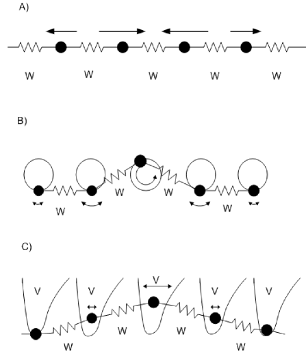
FIG. 1.: A schematic representation of different types of discrete breathers: a) acoustic breather; b) acoustic rotobreather; c) optical breather.

Although DBs present complex dynamical objects, in many cases experimental measurements can be well understood by using certain time-averaged properties of DBs [25, 26]. Thus, a natural question appears whether the internal breather dynamics is of crucial importance to understand the lattice dynamics in the presence of DBs. In this paper we study the propagation of small amplitude plane waves in one-dimensional nonlinear lattices in the presence of a DB and obtain that the internal dynamics of the DB may lead to a drastical increase or decrease of wave transmission as compared to the time-averaged setup. Thus the wave scattering by DBs is interesting both as some spectroscopical tool to study DB properties and as a way to control the wave transmission (conductivity) by varying the DB state. Finally our studies are of use for the general understanding of wave scattering by time-periodic potentials.

First successful attempts to describe the variety of phenomena arising from wave scattering by DBs have been performed some time ago [27, 28, 29, 30, 16]. While a number of results have been obtained, we are far from a full description of the complexity of possible scattering outcomes. This concerns the wave scattering in systems with acoustic spectra $\omega_{q}$, the importance of the internal DB dynamics including the comparison between rotational and vibrational excitations, the dependence of the wave propagation on the DB energy, and the single channel elastic versus the two channel inelastic scattering cases[28]. Here we will address these problems but restrict ourselves to the elastic scattering case.

The paper is organized as follows: in Section II we present the general formalism and describe analytical and novel numerical methods used to analyze the wave scattering by DBs, in Sections III, IV and V the dependencies of the transmission coefficient on the breather frequency $\Omega_{b}$ and the wave number $q$ for different types of breathers (acoustic breathers and rotobreathers, optical breathers, see Fig. 1) are obtained, and finally a discussion is provided in Section VI.

II General formalism

To proceed we will consider one-dimensional nonlinear lattices with nearest neighbor interaction, optional on-site (substrate) potential, and with one degree of freedom per lattice site. Both the increasing of the interaction range and the extension to more than the one degree of freedom per lattice site are not of crucial importance.

The dynamics of the system is characterized by time-dependent coordinates $x_{n}(t)$ and the class of Hamiltonians considered here reads

$${\mathrm{H}}=\sum_{n}\left(\frac{\dot{x}_{n}^{2}}{2}+V[x_{n}]+W[x_{n}-x_{n-1}]\right)\;.$$ (1)

Here $V[x]$ is an optional on-site (substrate) potential and $W[x]$ is the nearest neighbor interaction. The equations of motion become

$$\ddot{x}_{n}=-W^{\prime}[x_{n}-x_{n-1}]+W^{\prime}[x_{n+1}-x_{n}]-V^{\prime}[x_{n}]~{}~{}.$$ (2)

Without loss of generality we take $V[0]=W[0]=V^{\prime}[0]=W^{\prime}[0]=0$ and $V^{\prime\prime}[0]\geq 0$, $W^{\prime\prime}[0]>0$. This Hamiltonian supports the excitation of small amplitude linear waves with the frequency spectrum

$$\omega_{q}^{2}=V^{\prime\prime}[0]+4W^{\prime\prime}[0]\sin^{2}\left(\frac{q}{2}\right)~{}~{},$$ (3)

with $q$ being the wave number.

Time-dependent spatially localized solutions (DBs) exist for different types of potentials $V[x]$ and $W[x]$, although at least one of the two functions ($V[x]$ and/or $W[x]$) has to be anharmonic. DB solutions are characterized by being time-periodic $\hat{x}_{n}(t+T_{b})=\hat{x}_{n}(t)$ and spatially localized $\hat{x}_{|n|\rightarrow\infty}\rightarrow 0$ (except systems with $V=0$ where $\hat{x}_{n\rightarrow\pm\infty}\rightarrow\pm c$ with $c$ possibly being nonzero). If the Hamiltonian $H$ is invariant under a finite translation (rotation) of any $x_{n}\rightarrow x_{n}+\lambda$, then discrete rotobreathers (DRB) may exist [31]. These excitations are characterized by one or several sites in the breather center evolving in a rotational state $\hat{x}_{0}(t+T_{b})=\hat{x}_{0}(t)+\lambda$, while outside this center the lattice is governed again by time periodic spatially localized oscillations. The breather frequency $\Omega_{b}=2\pi/T_{b}$ can generally take any values provided $k\Omega_{b}\neq\omega_{q}$ for all nonzero integer $k$. As $\omega_{q}^{2}$ is an analytic function of $q$, DBs are exponentially localized on the lattice.

A The linearized problem

To study the scattering of small amplitude plane waves by a DB we linearize the equations of motion (2) around a breather solution $x_{n}(t)=\hat{x}_{n}(t)+\epsilon_{n}(t)$:

$$\ddot{\epsilon}_{n} = -W^{\prime\prime}[\hat{x}_{n}(t)-\hat{x}_{n-1}(t)](\epsilon_{n}-\epsilon_{n-1})$$ (5)

$$+W^{\prime\prime}[\hat{x}_{n+1}(t)-\hat{x}_{n}(t)](\epsilon_{n+1}-\epsilon_{n})-V^{\prime\prime}[\hat{x}_{n}(t)]\epsilon_{n}\;.$$

This is a set of coupled linear differential equations with time periodic coefficients of period $T_{b}$. Note that these coefficients are determined by the given DB solution $\hat{x}_{n}(t)$.

Eq.(5) determines the linear stability of the breather through the spectral properties of the Floquet matrix,[19, 28] which is given by a map over one breather period

$$\left(\begin{array}[]{l}\vec{\epsilon}(T_{b})\\ \dot{\vec{\epsilon}}(T_{b})\end{array}\right)={\mathbf{F}}\left(\begin{array}[]{l}\vec{\epsilon}(0)\\ \dot{\vec{\epsilon}}(0)\end{array}\right),$$ (10)

where $\vec{\epsilon}\equiv(...,\epsilon_{n-1},\epsilon_{n},\epsilon_{n+1},...)$. For marginally stable breathers all eigenvalues of the symplectic matrix ${\mathbf{F}}$ will be located on the unit circle and can be written as $e^{i\theta}$. The corresponding eigenvectors are the solutions of Eq.(5), and fulfill the Bloch condition

$$\epsilon_{n}(t+T_{b})=e^{-i\theta t/T_{b}}\epsilon_{n}(t)\;.$$ (11)

Because the DB solution is exponentially localized on the lattice, equation (5) will reduce to the usual small amplitude wave equation far away from the breather center. Thus, only a finite number of Floquet eigenvectors are spatially localized, while an infinite number of them (for an infinite lattice) are delocalized and these solutions correspond to plane waves with the spectrum (3) and the Floquet phases $\theta=\pm\omega_{q}T_{b}$. The remaining Floquet eigenvalues correspond to local Floquet eigenvectors and are separated from the plane wave spectrum on the unit circle. Note here, that two eigenvectors with the degenerated eigenvalue $e^{i\theta}~{}=~{}+1$ always exist and reflect perturbations tangent to the breather family of solutions.

As a consequence of the Bloch condition (11) any spatially extended Floquet eigenvector can be represented in the form

$$\epsilon_{n}(t)=\sum_{k=-\infty}^{\infty}e_{nk}{\rm e}^{{\rm i}(\omega_{q}+k\Omega_{b})t}.$$ (12)

What happens if we send a plane wave with frequency $\omega_{q}$ to the DB? We will deal with the case of one-channel scattering as for any $k\neq 0$ and any $q^{\prime}$, $\omega_{q^{\prime}}\neq\omega_{q}+k\Omega_{b}$. This condition determines that all channels with nonzero $k$ are ’closed’, i.e. the spatial amplitudes $e_{nk}$ are localized in space. Note here, that the frequencies of transmitted and reflected waves are the same and coincide with the the frequency of the incoming wave, since they all belong to the only open channel with $k=0$.

For harmonic interaction potentials $W$ it was shown in Ref. [28] that the momentum

$$J=-W^{\prime\prime}[0]\langle{\rm Im}\epsilon^{*}_{n}\epsilon_{n-1}\rangle$$ (13)

is independent of the lattice site. Here the averaging is meant with respect to time. In a similar way it is straightforward to show that the quantity

$$\tilde{J}=-\langle W^{\prime\prime}[\hat{x}_{n}(t)-\hat{x}_{n-1}(t)]{\rm Im}\epsilon^{*}_{n}\epsilon_{n-1}\rangle$$ (14)

is independent of the lattice site. Since the breather solution $\hat{x}_{n}(t)$ is spatially localized, at large distances from the breather we find again that the momentum $J$ is independent of the lattice site. Especially we find that it is the same for $n\rightarrow\pm\infty$. Following Ref. [28] we conclude that the one-channel scattering case is elastic, i.e. the energy of an incoming wave equals the sum of the energies of the outgoing (reflected and transmitted) waves.

Despite the fact that we will study the one-channel elastic scattering, the scattering potential of DB is time-periodic. The above mentioned ’closed’ channels are active inside the breather core, i. e. the frequency of linear waves in a finite area around the breather center can change due to the interaction with the DB (see Fig.2).

FIG. 2.: Schematic representation of the one-channel scattering of a wave by a discrete breather.

Thus one of the questions to be answered below is to identify the cases when the well-known scattering by a time-averaged (static) potential is not sufficient to describe the actual results of wave scattering by discrete breathers. This implies that interference effects through local interactions between the active closed channels may substantially change the scattering results as compared to a time-averaged scattering potential.

Assuming that the breather is located around the central site $n=0$, the one-channel scattering problem can be written as

$$\epsilon_{n}(t)=A_{I}e^{-i(\omega_{q}t+qn)}+A_{R}e^{-i(\omega_{q}t-qn)},~{}~{}n~{}<~{}0$$ (15)

$$\epsilon_{n}(t)=A_{T}e^{-i(\omega_{q}t-qn)}~{}~{},n~{}>~{}0$$ (16)

for

$$|n|\gg\sup[\xi_{b}(0),\xi_{b}(\omega_{q})]$$ (17)

where $\xi_{b}(\omega)=\sup\xi(\omega+k\Omega_{b})$ and

$$\begin{array}[]{l}\sinh^{2}\xi(\nu)/2=\frac{V^{\prime\prime}[0]-\nu^{2}}{4W^{\prime\prime}[0]}\;\;,\;\;|\nu|<\omega_{q}(0)\\ \cosh^{2}\xi(\nu)/2=\frac{\nu^{2}-V^{\prime\prime}[0]}{4W^{\prime\prime}[0]}\;\;,\;\;|\nu|>\omega_{q}(\pi)\end{array}$$ (20)

$\xi$ measures the characteristic inverse localization length of a closed channel at frequency $\nu$ (note that for $\nu=k\Omega_{b}$ the localization length is that of the breather itself, see also [28]). The incoming wave has amplitude $A_{I}$, and the reflected and transmitted wave amplitudes are given by $A_{R}$ and $A_{T}$ respectively. The transmission coefficient $t_{q}=\left|A_{T}/A_{I}\right|^{2}$.

For further considerations we will use the notation of the Bloch functions $\zeta_{n}(t)$ defined as

$$\epsilon_{n}(t)=\zeta_{n}(t)e^{-i\omega_{q}t}.$$ (21)

In order to estimate the relative strength of closed channels with $k\neq 0$ we expand the time-periodic coefficients of (5) in a Fourier series with respect to time:

$$W^{\prime\prime}[\hat{x}_{n}(t)-\hat{x}_{n-1}(t)]=\sum_{k=-\infty}^{\infty}w_{n,k}{\rm e}^{{\rm i}k\Omega_{b}t}\;,$$ (22)

$$V^{\prime\prime}[\hat{x}_{n}(t)]=\sum_{k=-\infty}^{\infty}v_{n,k}{\rm e}^{{\rm i}k\Omega_{b}t}\;.$$ (23)

We consider first the case of a strongly localized optical breather located at site $n=0$ with $W(y)=\frac{c}{2}y^{2}$. Taking into account a single closed channel with some value of $k$, inserting (22),(23) and (12) into (5) and excluding $e_{nk}$, the relative strength $s_{k}$ of the closed channel to the open one will be given by

$$s_{k}=\left|\frac{v_{0,k}^{2}}{(v_{0,0}-1)(v_{0,0}+2c(1-\eta_{k})-(\omega_{q}+k\Omega_{b})^{2})}\right|\;,$$ (24)

where the relative amplitude

$$\eta_{k}=\pm\frac{e_{1,k}}{e_{0,k}}={\rm e}^{-\xi(\omega_{q}+k\Omega_{b})}$$ (25)

has positive sign for $\omega_{q}+k\Omega_{b}$ located inside the phonon gap and negative sign otherwise. For $s_{k}\ll 1$ we do not expect any significant contribution from the given closed channel, while $s_{k}\geq 1$ indicate a strong influence of the closed channel on the scattering process. Note that the expression $\sqrt{v_{00}+2c(1-\eta_{k})}$ in the denominator of (24) is just a frequency $\omega_{L}$ of a local phonon mode of the time-averaged scattering potential. For spatially discrete systems these local phonon modes may be located inside or outside of the phonon gap. The denominator of (24) may vanish for certain wave numbers, which would imply a resonance-like enhancement of the closed channel contribution (for certain wavenumbers $q$). As such a resonant enhancement of a closed channel amplitude acts as a huge effective scattering potential to the open channel, for these cases we expect a resonant suppression of transmission. Thus, qualitatively such a complete suppression of transmission (Fano-like resonance [13, 15]) is explained by a resonant interaction of the propagating phonon with the specific local phonon mode. However in order to quantitatively analyze this effect the renormalization of the value of $\omega_{L}$ due to all nonresonant processes, has to be taken into account. It will be done below for a particular case of optical breathers by making use of the Green function method. We obtain that although the renormalization of $\omega_{L}$ is rather small it may become important especially as the width of a phonon band is small, $W^{\prime\prime}~{}\ll~{}1$.

In a similar way we proceed for the estimation of the closed channel contribution of acoustic breathers. We obtain the following expression for the relative strength $r_{k}$

$$r_{k}=\left|\frac{w_{0,k}^{2}}{(w_{0,0})(w_{0,0}-(\omega_{q}+k\Omega_{b})^{2})}\right|~{}~{}.$$ (26)

Thus, we again find a resonant suppression of transmission when the presence of acoustic DB leads to a local increase in the nearest neighbor interaction and to an appearance of a corresponding local phonon mode. However, this case is much more involved as compared to the optical DB case, and Eq. (26) may serve only as a qualitative tool to check whether a closed channel is strongly contributing to the transmission or not. We will instead provide with a more quantitative analysis for the cases considered, based on the particular acoustic breather properties.

B Numerical scheme

To compute numerically the transmission coefficient we have developed a scheme which generalizes the one given in Ref. [28] (which relies on a spatial reflection symmetry of the breather and thus of the scattering potential). At variance with Ref. [28] our scheme is capable of dealing with any (perhaps spatially nonsymmetric) time-periodic scattering potential.

We look for solutions of Eq.(5) which correspond to zeroes of the operator

$${\mathbf{G}}(\vec{\epsilon}(0),\dot{\vec{\epsilon}}(0))=\left(\begin{array}[]{c}\vec{\epsilon}(0)\\ \dot{\vec{\epsilon}}(0)\end{array}\right)-e^{i\omega_{q}T_{b}}\left(\begin{array}[]{c}\vec{\epsilon}(T_{b})\\ \dot{\vec{\epsilon}}(T_{b})\end{array}\right)$$ (31)

on a lattice with $2N+1$ sites labeled $-N,(-N+1),...,-1,0,1,...(N-1),N$. The incoming wave is fed from the left, and the transmitted wave is leaving the system to the right. The boundary condition at the right end is $\epsilon_{N+1}=e^{-i\omega_{q}t}$, which implies that the transmitted wave will have amplitude 1. With a given boundary condition at the left end $\epsilon_{-N-1}=(A+iB)e^{-i\omega_{q}t}$, where $A$ and $B$ are real numbers, we may find the zeroes of (31) using a standard Newton routine. Due to the linearity of the equations of motion in $\epsilon$ an arbitrary initial guess and one Newton step are needed to converge to the zeroes. In practice due to roundoff errors an additional Newton step may be required.

However with arbitrary $A$ and $B$ we will not realize the scattering case (15,16) in general. This is due to the fact that all extended Floquet states of an infinite system are twofold degenerated because time reversal symmetry holds far from the breather center. To succeed we add a second Newton procedure which uses $A$ and $B$ as free parameters such that the solution on site $N$ becomes $\epsilon_{N}=e^{-iq-i\omega_{q}t}$, ensuring that we realize a single transmitted traveling wave of amplitude one at the right end of the system. After the Newton procedures are completed, the transmission coefficient is then given by

$$t_{q}=\frac{4\sin^{2}q}{|(A+iB)e^{-iq}-\zeta_{-N}|^{2}}.$$ (32)

While the Bloch functions $\zeta_{n}$ are in general time-dependent close to the breather center, they will be time-independent complex numbers at large distance from the breather. We note that the computation operates at the machine precision, and we obtain results which are size independent, i.e. with the above described boundary conditions we emulate an infinite system. The discrete breather solution itself has to be obtained beforehand using standard numerical procedures [32].

The enumerator in (32) vanishes at the extremal values of $\omega_{q}$, i.e. at $q=0$ and $q=\pi$. If the denominator is finite at these values of $q$, the transmission will also vanish. This is indeed the generic case for a quadratic dependence of the spectrum $\omega_{q}$ on $q$ around these points. Exceptions are expected for acoustic chains (see next Section).

Another peculiar point is that if upon changing some control parameter, e.g. the breather frequency, a localized Floquet eigenstate attaches to or disattaches from the extended Floquet spectrum, the transmission coefficient will be exactly $t=1$ for the $q$-value which corresponds to the edge of the spectrum $\omega_{q}$, i.e. $q=0$ or $q=\pi$ [28, 29].

C Green function method for a time-periodic localized scattering potential

We will also analyze the wave propagation through DBs by making use of the Green function technique [33]. This method is especially convenient as the scattering potential is localized in space. To apply this method to a particular case when the presence of DBs leads to the appearance of a localized time-dependent on-site scattering potential, $V^{\prime\prime}[\hat{x}_{n}(t)]-1$, we perform a time Fourier transformation of Eq. (5) and obtain the equation for the Green function $G_{\omega_{q}}(n_{1},n_{2})$ :

$$G_{\omega_{q}}(n_{1},n_{2})~{}=~{}G^{0}_{\omega_{q}}(n_{1},n_{2})-$$

$$-\sum_{m}G^{0}_{\omega_{q}}(n_{1},m)\int d\Omega U_{\Omega}(m)G_{\omega_{q}+\Omega}(m,n_{2})~{}~{},$$ (33)

where $G^{0}_{\omega_{q}}(n_{1},n_{2})$ is the Green function of the linear equations of motion in the absence of the DB. The Fourier transform of the localized scattering potential $U_{\Omega}(m)~{}=~{}\int dte^{i\Omega t}(V^{\prime\prime}[\hat{x}_{m}(t)]-1)$ is determined by the properties of the DB solution. Because the DBs are periodic solutions in time the potential $U_{\Omega}(m)$ contains just the harmonics of the breather frequency, $\Omega~{}=~{}k\Omega_{b}$. Moreover, as we will see later in the considered cases we can take into account the harmonics with small values of $k~{}=0~{},\pm 1,~{}\pm 2$ only. Thus, the calculation of the Green function $G_{\omega_{q}}(n_{1},n_{2})$ can be represented in a diagrammatic form where terms which correspond to active closed channels describe the local (virtual) absorption and emission of phonons by the propagating phonon in the presence of the DB (some of the typical diagrams are shown in Fig.3). Moreover, for one-channel scattering the energy conservation law of absorbed and emitted phonons has to hold. In order to obtain the transmission coefficient $t_{q}$ we need also an expression for the Green function $G^{0}_{\omega}(n_{1},n_{2})$ which reads

$$G^{0}_{\omega}(n_{1},n_{2})~{}=~{}-\int\frac{dq}{2\pi}\frac{e^{iq(n_{1}-n_{2})}}{\omega^{2}-\omega_{q}^{2}}~{}~{}.$$ (34)

The Green function of the full problem (for one-channel scattering) has a similar form for large distances from the breather center ($n_{1}\rightarrow-\infty$ and $n_{2}\rightarrow+\infty$):

$$G_{\omega_{q}}(n_{1},n_{2})~{}=~{}-iD_{q}\frac{e^{iq|n_{1}-n_{2}|}}{d(\omega_{q}^{2})/dq}~{}~{},$$ (35)

where $t_{q}~{}=~{}|D_{q}|^{2}$.

As an example for a static scattering potential which is strongly localized on a single site ($n=0$) we obtain

$$G_{\omega_{q}}(n_{1},n_{2})~{}=~{}\frac{G_{\omega_{q}}^{0}(n_{1},n_{2})}{1+\beta_{0}G_{\omega_{q}}^{0}(0,0)}~{}~{},$$ (36)

where $\beta_{0}$ is the strength of the static potential. The transmission coefficient $\tilde{t}_{q}$ in this case is given by

$$\tilde{t}_{q}~{}=~{}\frac{(d(\omega_{q}^{2})/dq)^{2}}{\beta_{0}^{2}+(d(\omega_{q}^{2})/dq)^{2}}~{}~{}.$$ (37)

We will use the Green function method in Section V where the wave scattering by optical DBs (see Fig. 1c) will be presented. We show how most important diagrams can be taken into account in the case of a time-periodic localized scattering potential.

FIG. 3.: Typical diagrams describing the interaction of the propagating phonons with the time-periodic DB scattering potential: a) scattering by a time-average (static) potential; b) resonant scattering process; c) a process leading to the renormalization of a phonon local mode frequency; d) various complex processes. Here, thin and thick solid lines present the Green functions in the absence of the DB and in the presence of the time-average part of the DB scattering potential. The time-average part of the DB scattering potential is shown by a black circle, and the dashed lines show the absorption (emission) of phonons.

D Time-averaged scattering potential

Since we are interested in understanding the importance of the time dependence of the scattering potential, we will also compare the numerical results with those obtained by time-averaging the DB scattering potential. This time-averaging can be found numerically beforehand and Eq. (5) becomes

$$\ddot{\tilde{\epsilon}}_{n} = -w_{n,0}(\tilde{\epsilon}_{n}-\tilde{\epsilon}_{n-1})+$$ (39)

$$w_{n+1,0}(\tilde{\epsilon}_{n+1}-\tilde{\epsilon}_{n})-v_{n,0}\tilde{\epsilon}_{n}.$$

Because in this case all inhomogeneities are time-independent we can use the standard scattering matrix method. With $\tilde{\epsilon}_{n}(t)=\tilde{\zeta}_{n}e^{-i\omega_{q}t}$ Eq.(39) is rewritten as

$$\left(\begin{array}[]{l}\tilde{\zeta}_{n+1}\\ \tilde{\zeta}_{n}\end{array}\right)={\mathbf{M}}_{n}\left(\begin{array}[]{l}\tilde{\zeta}_{n}\\ \tilde{\zeta}_{n-1}\end{array}\right),$$ (44)

with

$${\mathbf{M}}_{n}=\left(\begin{array}[]{cc}1+\frac{E_{n}+c_{n,n-1}-\omega_{q}^{2}}{c_{n+1,n}}&-\frac{c_{n,n-1}}{c_{n+1,n}}\\ 1&0\end{array}\right)$$ (47)

where $E_{n}=v_{n,0}$ and $c_{n,n-1}=w_{n,0}$. It follows

$$\left(\begin{array}[]{l}\tilde{\zeta}_{N+1}\\ \tilde{\zeta}_{N}\end{array}\right)={\mathbf{M}}\left(\begin{array}[]{l}\tilde{\zeta}_{-N}\\ \tilde{\zeta}_{-N-1}\end{array}\right),$$ (52)

with

$$\mathbf{M}=\prod\limits^{-N}_{i=N}\mathbf{M}_{i}.$$ (53)

The expression for the transmission coefficient $\tilde{t}_{q}$ for the time averaged scattering potential is then given by

$$\tilde{t}_{q}=\frac{4\sin^{2}q}{|M_{11}(q)e^{-iq}+M_{12}(q)-M_{21}(q)-M_{22}(q)e^{iq}|^{2}}$$ (54)

where $M_{ij}$ are the four matrix elements of the $2\times 2$ matrix $\mathbf{M}$.

III Scattering by acoustic breathers

In this Section we study the wave scattering by so-called acoustic breathers. The corresponding systems are characterized by a gapless spectrum $\omega_{q}$ of propagating linear waves, and by a conservation of total mechanical momentum.

The generic choice for the potentials in the Eq. (2) is $V(y)\equiv 0$ and $W(y)=\frac{1}{2}y^{2}+\frac{\beta}{3}y^{3}+\frac{1}{4}y^{4}$. This choice leads to the well known Fermi-Pasta-Ulam system [34]. We will first consider the case $\beta=0$ which implies the presence of a parity in the interaction potential $W$ and comment on the influence of parity violation for $\beta\neq 0$ later on. The dispersion relation of phonons is given by

$$|\omega_{q}|=2\sin\frac{q}{2}$$ (55)

A breather solution with frequency $\Omega_{b}=4.5$ is shown in Fig.4.

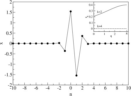
FIG. 4.: Displacements of an acoustic breather with zero velocities at $t=0$ and $\Omega_{b}=4.5$.
Inset: Relative strength $r_{k}$ for the second and fourth closed channels versus $q$.

The corresponding Fourier components of the scattering potential are plotted in Fig.5.

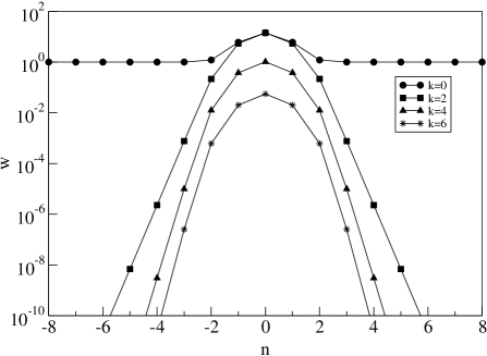
FIG. 5.: Fourier components $w_{nk}$ for different $k$ versus $n$ for the breather in Fig.4.

Acoustic breathers can be found with frequencies above the phonon band $|\Omega_{b}|>\max{|\omega_{q}|}$. However, here we consider $|\Omega_{b}|>2\max{|\omega_{q}|}$ which implies $|\Omega_{b}|>4$. This condition is needed to realize the one-channel scattering case of linear waves. For $\beta=0$ the ac part of the interaction potential $W$ has even harmonics only, and the frequency of a propagating phonon in a closed channel $2\Omega_{b}\pm\omega_{q}$ can not match the frequency of a local mode of the time-averaged scattering potential. Thus the closed channels play no important role in the scattering process. As a consequence the wave scattering by acoustic breathers is practically identical with the scattering by the time-averaged potential. Indeed numerical computations do not show any relevant difference between the linear wave propagation in the presence of time-dependent and the static (time-averaged) potentials. Yet there is a number of interesting features of the scattering which deserve to be exploited.

For $V=0$ the lattice conserves the total mechanical momentum $P=\sum_{n}\dot{x}_{n}$ in addition to the energy. Without loss of generality we will choose $P=0$ here. From this conservation law it follows that the total mechanical momentum of the linearized problem $\Pi=\sum_{n}\dot{\epsilon}_{n}$ is also conserved. This implies that for any solution $\epsilon_{n}(t)$ the shift $\epsilon(t)+C$ is also a solution. In particular $\epsilon_{n}=C$ is a solution, which corresponds to a wave with $q=0$ and for which we have $t_{q=0}=1$. Thus we conclude that the transmission of waves by a breather for acoustic systems at $q=0$ is always perfect, no reflection occurs. This is in sharp contrast to systems without conservation of total mechanical momentum (see below).

The peculiar dependence of the transmission coefficient $t_{q}$ on the wave number $q$ and the breather frequency $\Omega_{b}$ is shown in Fig.6. The breather frequency is varying over nearly three decades. We indeed observe perfect transmission at $q=0$, and zero transmission at $q=\pi$. However we also find that in the studied breather frequency range two rather narrow peaks around $q=\pi$ appear with perfect transmission. These structures are due to the detachment of localized Floquet eigenvectors from the continuum of extended Floquet eigenstates. A surprising result is shown in Fig.7. We plot the transmission $t_{q}$ at $q=\pi/4$ as a function of the breather frequency $\Omega_{b}$. We obtain plateaus and crossovers at certain breather frequencies. The crossover positions clearly correlate with the appearance of localized Floquet states, which are traced through the perfect transmission close to $q=\pi$ in Fig.6. The dependence of the transmission on $q$ for the two observed plateaus is shown in the inset of Fig.7. The plateaus range over several decades in $\Omega_{b}$, and the $q$-dependence of $t_{q}$ is rather similar on different plateaus.

To understand this feature we remind that large breather frequencies imply that the breather energy and its amplitude in the breather center are large as well. Thus we may neglect the harmonic part of the interaction potential $W$ inside the breather core. The resulting amplitude distribution of the breather core is characterized by a superexponential decay $\hat{x}_{n}(t)=A_{n}G(t)$, $A_{n}\sim A_{n-1}^{3}$, where $G(t)$ is an oscillatory master function [35, 36]. Due to the symmetry of the breather solution the spatial profile is described by $A_{-n}=-A_{n+1}\;,\;n\leq 0$. The amplitudes $A_{n}$ have been computed: $A_{1}=1$, $A_{2}~{}\simeq~{}-0.166$, $A_{3}~{}\simeq~{}4.796~{}10^{-4}$, $A_{4}~{}\simeq~{}-1.15~{}10^{-11}$, and so on [34]. The overall amplitude of the oscillations $\hat{x}_{n}(t)$ is tuned by the amplitude of the master function $G(t)$.

The scattering is essentially described by the time-averaged scattering potential. This potential corresponds to a large increase in the nearest neighbour coupling terms. In the breather center we find

$$\langle W^{\prime\prime}[\hat{x}_{1}(t)-\hat{x}_{0}(t)]\rangle=1+3\langle(\hat{x}_{1}(t)-\hat{x}_{0}(t))^{2}\rangle$$ (56)

with

$$3\langle(\hat{x}_{1}(t)-\hat{x}_{0}(t))^{2}\rangle\equiv X^{2}\approx\frac{2}{3\pi}\Omega_{b}^{2}$$ (57)

(the details of the calculation are presented in Appendix A). Due to the large value of $X$ for large $\Omega_{b}$ it becomes evident that time-dependent corrections to the scattering potential are negligible. By making use of the distribution of oscillation amplitudes in the lattice we then find

$$3\langle(\hat{x}_{n}(t)-\hat{x}_{n-1}(t))^{2}\rangle\approx A_{n}^{2}X^{2}.$$ (58)

The scattering on a plateau in Fig.7 is due to a finite number of matrices $\mathbf{M}_{n}$ which should be taken into account in Eq. (53). Qualitatively the crossover threshold can be defined as

$$A_{n}^{2}X^{2}\simeq 1~{}~{}.$$ (59)

Thus we obtain the two crossover frequencies $\Omega_{b1}=13.1$ and $\Omega_{b2}=4527$, which match with the observed crossover positions. For $4<\Omega_{b}<\Omega_{b1}$ we need only 4 matrices $\mathbf{M}_{n}$, for $\Omega_{b1}<\Omega_{b}<\Omega_{b2}$, 6 matrices $\mathbf{M}_{n}$ and so on. We also computed the transmission at $q=\pi/4$ using the corresponding reduced set of relevant matrices. The obtained limiting values of $t_{q}$ are shown as a dashed line in Fig.7. We observe very good agreement between the predicted plateau heights and the actual data obtained in direct numerical simulations.

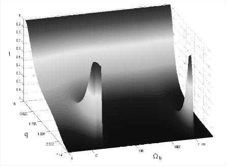
FIG. 6.: The dependence of the transmission coefficient on $q$ and $\Omega_{b}$.

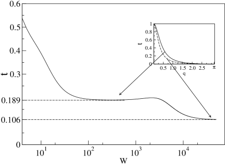
FIG. 7.: The dependence of the transmission coefficient on $\Omega_{b}$ for a particular value of $q=\frac{\pi}{4}$. The dashed lines show the predicted plateau heights (see text). The inset shows the dependence of the transmission on $q$ for the two observed plateau regions.

With the above said it becomes also transparent, why we observe detachment of localized Floquet states in the crossover region. The acoustic breather presents an effective potential well for the propagating phonons. The width of this well increases with the breather frequency, and the number of possible localized Floquet states also increases. Such a periodic appearance of perfect transmission is similar to the quantum mechanical scattering by a potential well in the presence of quasi-discrete levels [37].

Finally we checked the influence of $\beta\neq 0$. With respect to the breather the presence of cubic terms in the interaction potential leads to the generation of a kink-shaped dc lattice distortion. The corresponding scattering potential becomes asymmetric in space and odd harmonics in the ac scattering potential appear. This immediately leads to the possibility of matching between the frequency of a propagating phonon in a closed channel $\Omega_{b}-\omega_{q}$ and several local modes of the time-averaged scattering potential. Thus, a resonant suppression of a transmission appears in this case. Indeed, we observe this effect by direct numerical simulations as shown in Fig.8, where two transmission zeros are found. We will discuss this effect in more detail for the case of optical breathers below.

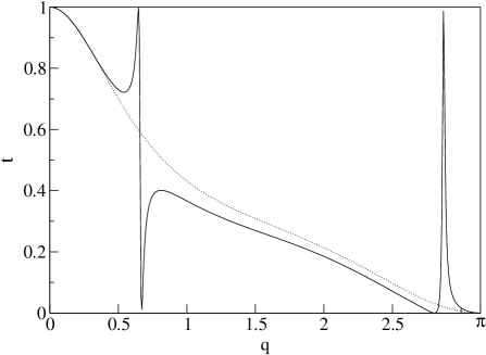
FIG. 8.: The dependence of the transmission coefficient on $q$ for an acoustic breather with $\Omega_{b}=4.5$ and $\beta=1$. The dashed line is the result for the time-averaged scattering potential. Two transmission zeros are observed at corresponding values of $q$.

IV Scattering by acoustic rotobreathers

Remarkable differences to the results of the preceding Section are obtained if the interaction potential $W$ is chosen to be a periodic one (the potential $V$ is still zero in this Section):

$$W(y)=1-\cos(y).$$ (60)

With such an interaction potential the nonlinear chain allows for the existence of rotobreathers (cf. Fig.1b). In the simplest case a rotobreather consists of one particle being in a rotating (whirling) state, while all others particles with spatially decaying amplitudes from the center of DB:

$$\hat{x}_{0}(t+T_{b})=\hat{x}_{0}(t)+2\pi,$$ (61)

$$\hat{x}_{n\neq 0}(t+T_{b})=\hat{x}_{n\neq 0}(t),$$ (62)

$$\hat{x}_{|n|\rightarrow\infty}\rightarrow 0.$$ (63)

To excite such a rotobreather the central particle needs to overcome the potential barrier generated by its two nearest neighbors. The rotobreather energy is thus bounded from below by $E_{b}>4$. At sufficiently large energies $E_{b}\gg 4$ the central particle will perform nearly free rotations $\hat{x}_{0}(t)=\Omega_{b}t+\delta(t)$ with $\delta(t+T_{b})=\delta(t)$ being a small correction. The time-averaged off-diagonal hopping terms between site $n=0$ and $n=\pm 1$ are then given by

$$\langle\cos(\hat{x}_{0}(t)-\hat{x}_{1}(t))\rangle\approx-\langle\sin(\Omega_{b}t)(\delta(t)-\hat{x}_{1}(t))\rangle$$ (64)

where $\hat{x}_{1}(t)$ is also a small function. Thus the time-averaged scattering potential of a rotobreather presents a huge barrier that cuts the chain into nearly noninteracting parts, contrary to the previous case of an acoustic breather, where the acoustic breather potential corresponds to a potential well. Therefore it becomes extremely difficult for waves to penetrate across the rotobreather. The rotobreather solution with $\Omega_{b}=4.5$ is shown in Fig.9.

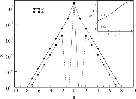
FIG. 9.: Displacements and velocities of an acoustic rotobreather at $t=0$ with $\Omega_{b}=4.5$.
Inset: Relative strength $r_{k}$ for the first and second closed channels versus $q$.

The corresponding Fourier components of the scattering potential are shown in Fig.10.

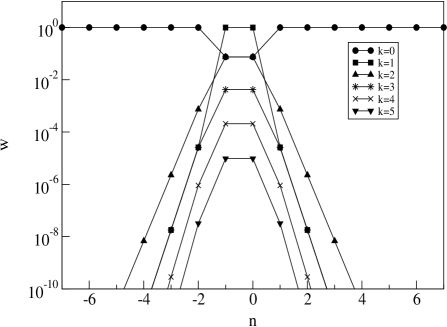
FIG. 10.: Fourier components $w_{nk}$ for different $k$ versus $n$ for the rotobreather in Fig.9.

In Fig.11 we show the $q$-dependence of the transmission for a rotobreather with $\Omega_{b}=4.5$ and compare it to the corresponding curve of an acoustic breather from the preceding section. We observe a dramatic decrease of the transmission at all $q$-values for the rotobreather, in agreement with the above analysis.

To decide whether the time-dependence of the rotobreather scattering potential is important or not, we first make a more precise computation for (64) (details of the calculations are presented in Appendix B)

$$\langle\cos(\hat{x}_{0}(t)-\hat{x}_{1}(t))\rangle\approx-\frac{3}{2\Omega_{b}^{2}}.$$ (65)

The time-averaged scattering potential for large $\Omega_{b}$ corresponds to two neighboring weak links of strength (65) inserted in a linear acoustic chain. Three matrices $\mathbf{M}_{n}$ are enough to compute the transmission. Two of them involve matrix elements which are proportional to $\Omega_{b}^{2}$. The elements of the product will thus contain terms proportional to $\Omega_{b}^{4}$, and according to (54) the result is

$$\tilde{t}_{q}\sim\Omega_{b}^{-8}.$$ (66)

This is precisely what we also find from a numerical evaluation of the transmission for the time-averaged scattering potential in Fig.12. However, although the transmission coefficient $t_{q}$ for the full time-dependent scattering potential also drastically decreases with $q$ and $\Omega_{b}$, the dependence is weaker than for the case of time-average rotobreather potential. It scales as

$$t_{q}\sim\Omega_{b}^{-4}$$ (67)

(see also Fig.12). The reason is that besides a weak static link the rotobreather scattering potential has an ac term at frequency $\Omega_{b}$ of amplitude one (see Fig.10). Thus an alternative route for the wave is to approach the rotobreather, to be excited into the first closed channel, to pass the breather and to relax back into the open channel. The corresponding scattering process of ”virtual” absorption and emission of phonons from the rotobreather can be also represented by three matrices as it happens for the dc analysis. However now instead of two weak links we have links of order one with a frequency change at site $n=0$ from $\omega_{q}$ to $\omega_{q}+\Omega_{b}$. This occurs in exactly one of the three matrices. Consequently the product matrix will contain elements proportional to $\Omega_{b}^{2}$ and the transmission will scale as (67).

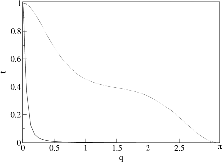
FIG. 11.: The dependence of the transmission coefficient on $q$ for $\Omega_{b}=4.5$. Data for acoustic rotobreather and acoustic breather are shown correspondingly by solid and dashed lines.

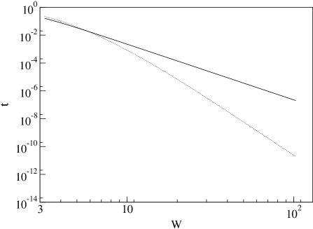
FIG. 12.: The dependence of the transmission coefficient on the frequency of the breather $\Omega_{b}$ at fixed $q=0.21$. Scattering by ”real” rotobreather and a static part of DB are shown correspondingly by solid and dashed lines.

We conclude this section by stressing that the wave scattering by an acoustic rotobreather is essentially relying on the time-dependence of the scattering potential. The rotobreather effectively cuts the chain in weakly interacting parts and thus hinders waves from propagation in a very strong way.

V Optical breathers

In this Section we consider systems with a nonvanishing on-site potential $V[x_{n}]\not=0$ (see Fig. 1c). The difference of such systems to acoustic models is the existence of a gap in the spectrum of phonons $|\omega_{q=0}|=V^{\prime\prime}[0]$. As a consequence the total mechanical momentum is not conserved, and the transmission coefficient now vanishes not only at $q=\pi$ but also at $q=0$. An exception is the case when a localized Floquet eigenstate bifurcates from the corresponding band edge for some special parameters [28, 29, 30]. Because of the presence of a gap in the plane wave spectrum there are now two different cases of interest - the breather frequency being located outside the spectrum $|\Omega_{b}|>\max{|\omega_{q}|}$ or inside the gap $|\Omega_{b}|<\min{|\omega_{q}|}$.

A The case $|\Omega_{b}|>\max{|\omega_{q}|}$.

Here we choose $V(y)=\frac{1}{2}y^{2}+\frac{1}{3}y^{3}+\frac{1}{4}y^{4}$ and $W(y)=\frac{c}{2}y^{2}$.

In this case the spectrum of phonons is

$$\omega_{q}^{2}~{}=~{}1+4c\sin^{2}(\frac{q}{2})~{}~{}.$$ (68)

The breather profile for $\Omega_{b}=1.5$ and $c=0.05$ is shown in Fig.13.

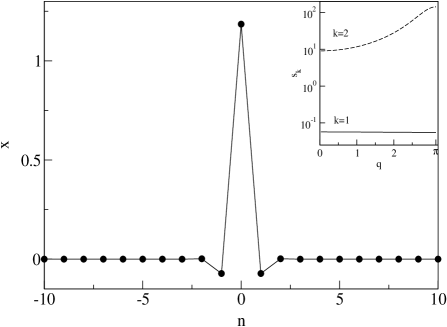
FIG. 13.: The initial displacements of an optical breather with $\Omega_{b}=1.5$ and $c=0.05$ (velocities are zero).
Inset: $s_{k=1,2}$ versus $q$.

The corresponding Fourier components of the scattering potential are plotted in Fig.14.

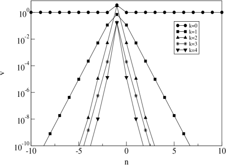
FIG. 14.: Fourier components $v_{nk}$ for different $k$ versus $n$ for the breather in Fig.13.

We note that the DB scattering potential perturbs the diagonal terms and in this particular case ($\Omega_{b}>\omega_{q}$) presents a barrier for propagating phonons. For large breather frequencies the breather is strongly localized, i.e. essentially only one central oscillator is excited. The time-averaged scattering potential then becomes a single diagonal defect with a large strength $\beta_{0}~{}\simeq~{}\Omega_{b}^{2}$. It is straightforward to observe that the transmission coefficient will thus scale as (see Eq.(37))

$$\tilde{t}_{q}\sim\Omega_{b}^{-4}.$$ (69)

Due to the fact that the transmission vanishes exactly for both $q=0$ and $q=\pi$ we conclude that for large breather frequencies transmission is suppressed in general.

However, in the case of an optical DB the time-dependent part of the DB scattering potential (more precisely its second harmonic, see Fig. 14 ) is also large as $\beta_{2}~{}\simeq~{}\Omega_{b}^{2}$ for large values of the breather frequency. Thus, the time-dependent part of the DB potential can be rather important. Indeed, for the breather from Fig.13 the obtained transmission as a function of $q$ shows that $\tilde{t}_{q}$ (see Fig.15, dashed line) is at least one order of magnitude larger than $t_{q}$ (see Fig.15, solid line). In addition $t_{q}$ shows a resonant minimum around $q=2.1$ (see inset). Let us use the estimation (24) for $k=1,2$. The parameters are $v_{0,0}=3.5\;,\;v_{0,1}=0.69\;,\;v_{0,2}=3$. First we find that $s_{1}\approx 0.05$ for all $q$ implying that the $k=1$ closed channel does not participate in the transmission process. At the same time $s_{2}>10$ for all $q$ and thus, the $k=2$ closed channel strongly participates in the transmission process. It is because the frequency of the propagating phonon $2\Omega_{b}-\omega_{q}~{}\simeq~{}1.92$ is close to a localized eigenmode of the time-averaged scattering potential $\omega_{L}~{}=~{}1.9$. Notice here that the frequency of this local mode is above the phonon band. Thus we interprete the suppression of transmission as a strong coupling between the propagating wave and a particular localized mode of the time-averaged scattering potential, mediated by the ac terms of the scattering potential (the $k=2$ channel in this case). However, the simple estimation based on Eq. (24) does not show the resonant suppression of transmission for a particular value of $q$ and therefore, in order to quantitatively describe this effect we next apply the Green function method.

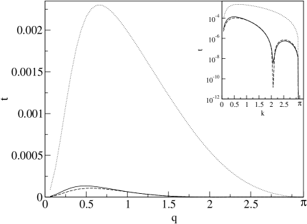
FIG. 15.: The dependence of the transmission coefficient $t_{q}$ on the wave number $q$. The optical breather frequency is $\Omega_{b}=1.5$ and the coupling $c=0.05$. The results are shown for the time-averaged DB scattering potential (dotted line); the time averaged part and the second harmonic of the DB scattering potential (dashed line); the full DB scattering potential (solid line).
Inset: same with $t_{q}$ on a logarithmic scale. Note the resonant suppression around $q=2.1$.

By making use of the estimation (24) we take into account in (33) the terms with $k=0$ and $k=\pm 2$, i. e. the scattering on the static potential and the phonon interaction with the second harmonic of the frequency $2\Omega_{b}$. Moreover, we use the fact that the DB scattering potential is a strongly localized one, and obtain (the corresponding diagram is shown in Fig. 3b)

$$G_{\omega_{q}}(n_{1},n_{2})~{}=~{}\tilde{G}_{\omega_{q}}(n_{1},n_{2})+$$

$$+\beta_{2}^{2}\tilde{G}_{\omega_{q}}(n_{1},0)\tilde{G}_{-\Omega+\omega_{q}}^{(rn)}(0,0)G_{\omega_{q}}(0,n_{2})~{}~{},$$ (70)

where $G_{\omega_{q}}(n_{1},n_{2})$ is determined by $\tilde{G}_{\omega}(n_{1},n_{2})$ that is the Green function of propagating phonons in the presence of time-average DB potential (the corresponding diagram is shown in Fig. 3a):

$$\tilde{G}_{\omega}(n_{1},n_{2})~{}=~{}G^{0}_{\omega}(n_{1},n_{2})-\beta_{0}G^{0}_{\omega}(n_{1},0)\tilde{G}_{\omega}(0,n_{2})~{}~{}.$$ (71)

Moreover, the central part of Eq. (70), namely $\tilde{G}_{-\Omega+\omega_{q}}^{(rn)}(0,0)$, has a resonant form:

$$\tilde{G}_{-\Omega+\omega_{q}}^{(rn)}(0,0)~{}=~{}\frac{1}{\omega_{L}^{2}-(\Omega-\omega_{q})^{2}}~{}~{},$$ (72)

where the local phonon mode frequency $\omega_{L}$ is mostly determined by a time-average scattering potential. However, in the case as the phonon band is narrow ($c~{}\ll~{}1$) the renormalization of $\omega_{L}$ due to the ac nonresonant processes has to be taken into account (the corresponding diagram is shown in Fig. 3c). The Eqs. (70) and (71) can be solved and we obtain

$$G_{\omega_{q}}(0,n_{2})~{}=~{}\frac{G^{0}_{\omega_{q}}(0,n_{2})}{1+(\beta_{0}-\beta_{2}^{2}\tilde{G}_{-\Omega+\omega_{q}}^{(rn)}(0,0))G^{0}_{\omega_{q}}(0,0)}~{}~{}.$$ (73)

Thus, we arrive at the expression (37) for the transmission coefficient $t_{q}$ but with the renormalized wave number dependent parameter $\beta$

$$\beta~{}=~{}\beta_{0}-\frac{\beta_{2}^{2}}{\omega_{L}^{2}-(2\Omega_{b}-\omega_{q})^{2}}.$$ (74)

As the breather frequency is large ($\Omega_{b}~{}\gg~{}1$) both transmission coefficients for the static DB scattering potential and for the full time-periodic DB scattering potential, decrease with the breather frequency according to (69). However, the effective potential strength $|\beta|$ is larger than $\beta_{0}$ and correspondingly the transmission $t_{q}$ is smaller compared to the transmission on the static DB scattering potential. Indeed, we observed this behaviour by direct numerical simulations (see Fig. 16).

A most peculiar effect is that the presence of ac term in a scattering potential allows to tune the frequency of a local mode and to obtain the resonant suppression of transmission. Indeed by taking into account the type of diagrams shown in Fig. 3c we obtain for the renormalized local mode frequency $\tilde{\omega}_{L}$

$$\tilde{\omega}_{L}^{2}~{}=~{}\omega_{L}^{2}+\frac{\beta_{2}^{2}}{(4\Omega_{b}-\omega_{q})^{2}-\omega_{L}^{2}}~{}~{}.$$ (75)

This formula is valid in the limit $\beta_{2}~{}\leq~{}2\sqrt{2}\Omega_{b}$ [38]. For the particular case of the DB with frequency $\Omega_{b}~{}=~{}1.5$ and $\beta_{2}~{}=~{}v_{02}/2~{}=~{}1.5$ we find that the resonant value of $q~{}\simeq~{}2$ is remarkably close to the resonant suppression of $t_{q}$ around $q~{}=~{}2.1$. Thus a strong dependence of $\omega_{L}$ on the amplitude of the ac part of DB scattering potential, and therefore, on the breather frequency, allows easily to change a position of the resonance.

Note here, that taking into account the static part and the second harmonic of the DB potential allows to obtain a good agreement with the direct numerical simulations of a scattering by the ”full” DB (compare solid and dashed lines in Fig. 15). It is also interesting to mention that the static part and the first harmonic of the DB potential ($k~{}=~{}1$) lead to an increase of the transmission coefficient compared to the scattering by the time-averaged DB potential. It is just due to the interplay between the strengths of different channels of the scattering potential (see Eq. (74)).

Thus, we conclude that the presence of a closed channel allowing absorption and emission of phonons around the center of the breather leads to strong interference effects which are of destructive nature in the given example of optical breather.

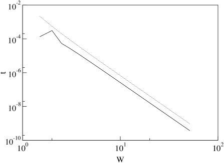
FIG. 16.: The dependence of the transmission coefficient $t_{q}$ on the optical breather frequency $\Omega_{b}$ for a particular value of wave number $q=0.5$. The dashed line corresponds to the scattering by a time-averaged DB scattering potential.

B The case $|\Omega_{b}|<\min{|\omega_{q}|}$

Here we choose the on-site potential in the form $V(y)=\frac{1}{2}y^{2}-\frac{1}{3}y^{3}$ (note here that the results do not change if the cubic term has a positive sign) and the interaction term $W(y)=\frac{c}{2}y^{2}$. The breather profile for $\Omega_{b}=0.85$ and $c=0.15$ is shown in Fig.17.

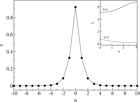
FIG. 17.: The initial displacements of an optical breather with $\Omega_{b}=0.85$ and $c=0.15$ (velocities are zero).
Inset: $s_{k=1,2}$ versus $q$.

The corresponding Fourier components of the scattering potential are plotted in Fig.18.

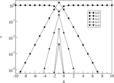
FIG. 18.: Fourier components $v_{nk}$ for different $k$ versus $n$ for the breather in Fig.17.

In this case the time-averaged DB scattering potential corresponds to a potential well in the diagonal terms, i. e. the parameter $\beta_{0}$ in Eq. (71) has a negative sign. It leads again to the possibility to obtain a resonance as the frequency of an active closed channel matches the frequency of a localized phonon mode located in the phonon gap. Moreover, at variance to the optical DB with large frequency (preceding subsection), the number of active closed channels may now increase substantially. This leads to a more complicated interference scenario between the open channel and several closed channels. Indeed, the estimation of $s_{k=1,2}$ shows that the first channel is strongly contributing, and the second closed channel can not be neglected either. At variance to the previous case for all propagating phonon frequencies the $k=1$ closed channel has a much stronger contribution than the $k=2$ one. However, we expect a resonant coupling between the propagating wave and the local mode through the $k=2$ closed channel, as $|\omega_{q=0}-2\Omega_{b}|=0.7$ is close to a local eigenmode of the time-averaged scattering potential with frequency $\omega_{L}=\pm 0.78$. Moreover, the nonresonant processes in a strong $k=1$ channel allow to renormalize $\omega_{L}$ similarly to the previous case of an optical breather with a large frequency. This resonant effect can be analyzed by making use of Eqs. (37), (70)-(74). Indeed, due to the resonance with a localized phonon mode the Green function $\tilde{G}_{-2\Omega_{b}+\omega_{q}}^{(rn)}(0,0)~{}\gg~{}1$ for a particular wave number $q_{0}$. In this case the parameter $\beta$ goes to infinity as the resonant condition, $(2\Omega_{b}-\omega_{q_{0}})^{2}-\omega_{L}^{2}=0$, is valid and correspondingly the transmission coefficient vanishes. [39]. As the phonon frequency deviates from the resonant condition, the parameter $\beta$ decreases and correspondingly the transmission coefficient reaches a maximum (see Fig. 19).

In Fig.19 we show that the time-averaged DB scattering potential provides with perfect transmission at a certain wave number due to the presence of a quasi-bound state in the static scattering potential. At the same time the transmission for the full dynamical problem shows a maximum value of 0.1, and an additional minimum in $t(q)$ with actually a full vanishing of transmission. These patterns are entirely absent in the scattering by the time-averaged potential. Thus we again conclude that the presence of active closed channels inside the breather core leads to strong interference effects.

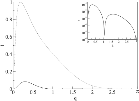
FIG. 19.: The numerically calculated dependence of the transmission coefficient $t_{q}$ (solid line) on $q$ for the breather frequency $\Omega_{b}=0.85$ and $c=0.15$. The dashed line shows the scattering by the time-averaged DB scattering potential. Inset: The same on a logarithmic scale.

VI Discussion

In this paper we considered the propagation of small-amplitude phonons through a nonlinear lattice in the presence of various discrete breathers. In particular, we obtained the transmission coefficient $t_{q}$ for the cases of acoustic and optical discrete breathers, and acoustic rotobreathers. We have shown that the presence of a DB leads to an effective scattering potential for phonons and this potential contains both static (time-averaged) parts and time-dependent periodic parts where the first and second harmonics are most important. Moreover, the strength and the width of the scattering potential are determined by the breather frequency $\Omega_{b}$.

The static part of the effective DB scattering potential may fully describe the scattering outcome if the closed channels weakly contribute (acoustic breather with $\beta=0$). Equally the leading contribution to a finite transmission may come from a closed channel (acoustic rotobreather). A very interesting case is realized when a local mode of the time-averaged scattering potential resonates with a closed channel (acoustic breather with $\beta\neq 0$, optical breathers). This resonance leads to a full suppression of transmission at some value of $q$. The nonresonant closed channels renormalize the local mode frequency and the corresponding position of the transmission zero in $q$. This effect has been discussed in several papers in relation to the Fano resonance [16, 40]. A detailed explanation of the similarities and differences to the physics of a Fano resonances is beyond the scope of this work and will be published separately. It is worthwhile to note here that the location of a zero transmission value in $q$ is not related to the presence of so-called quasi-bound Floquet states, i.e. states which by parameter tuning are transformed from a localized state into one colliding (interacting) with the continous part of the Floquet spectrum. Instead a formally exact definition of a zero transmission is given in [28] through the asymptotic phase properties of Floquet eigenstates far from the breather center.

The phonon scattering by inhomogeneities can be relevant with respect to the ongoing discussion about finite vs. infinite heat conductivity in acoustic chains with conservation of total mechanical momentum Ref. [7, 8, 9, 41]. The heat conductivity $\kappa$ mediated by noninteracting phonons is determined as

$$\kappa~{}\simeq~{}L\int dqT_{q}(L)~{},$$ (76)

where $L$ is the size of the system. Here $T_{q}(L)$ denotes the transmission of the given system. Thus, obviously in the absence of inhomogeneities the phonon heat conductivity goes to infinity ($\kappa~{}\simeq~{}L$) as the size of the system $L$ increases. However, the situation becomes more complex in the presence of inhomogeneities. In the case, when the inhomogeneities are randomly distributed along the system, the number of inhomogeneities $N=nL$, where $n$ is the concentration of defects, and the total transmission $T_{q}(L)~{}\simeq~{}t_{q}^{N}$ with $t_{q}$ being the transmission through a given defect. We obtain that the behaviour of heat conductivity is determined by the values of $q$ where $t_{q}$ is close to one. Thus, the problem of an infinite heat conductivity in the limit of a large size $L$ naturally appears in the systems preserving the total mechanical momentum.

In particular we can apply this general consideration to the phonon propagation in the presence of DBs. In the most interesting case of acoustic rotobreathers we obtain that the transmission coefficient $t_{q}~{}\simeq~{}1-\alpha q^{2}$ in the limit of small wave numbers. The coefficient $\alpha$ is determined by the frequency $\Omega_{b}$ and the specific choice of the acoustic rotobreather. Thus we argue that the mere presence of acoustic rotobreathers does not lead to a finite heat conductivity and $\kappa$ is still divergent in the limit of large $L$ as

$$\kappa~{}\simeq~{}\sqrt{\frac{L}{n\alpha}}~{}~{}.$$ (77)

Here we assume that the heat is carried by phonons, and did not take into account phonon-phonon interactions. Another conclusion drawn from our results for acoustic breathers versus acoustic rotobreathers is that the $q$-domain around $q=0$ where the transmission is close to one is by orders of magnitude smaller for acoustic rotobreathers as compared to acoustic breathers. This region is responsible for the quasiballistic transport of energy by large wavelength phonons in the hydrodynamic regime and for the appearance of anomalous heat conductivity. Numerical simulations for systems with acoustic rotobreathers have to be performed on length and time scales which are thus also orders of magnitude larger than the corresponding simulations for standard FPU chains.

Our analysis can be also applied to the electromagnetic wave propagation through various Josephson transmission lines. Although these systems are intrinsically dissipative, the dissipation may be rather small, and the transmission $t_{q}$ is still determined by the presence of inhomogeneities like rotobreathers [21, 22, 25, 26] or dynamic edge states[42]. Moreover, in this particular case of Josephson lattices the properties of DBs can be easily tuned experimentally by changing the external dc bias. Notice here that local phonon modes located on a rotobreather play an important role in various switching processes [26]. A study of an electromagnetic wave propagation may allow a direct observation of this mode.

Finally, a similar analysis can be carried out for a Schrödinger equation in the presence of artificially applied time-periodic perturbations [38]. This case is important for the description of electron transport through a quantum wire in the presence of external electromagnetic fields.


Acknowledgements
We thank S. Aubry, G. Casati, S. Kim and L. E. Reichl for useful discussions. This work was supported by the Deutsche Forschungsgemeinschaft FL200/8-1. M. V. F. thank the Alexander von Humboldt Stiftung for partial supporting this work.

A Time-averaged scattering potential for acoustic breather

We take into account the oscillations of two lattice sites in the center of a DB only. These oscillations evolve exactly in antiphase with large amplitudes. The effective Hamiltonian is written as

$$E=\frac{\dot{x}_{1}^{2}}{2}+\frac{\dot{x}_{2}^{2}}{2}+\frac{1}{4}(x_{1}^{4}+x_{2}^{4}+(x_{1}-x_{2})^{4})$$ (A1)

and with $x_{1}=-x_{2}$, we arrive at the single oscillator problem with energy

$$E=\dot{x}^{2}+\frac{9}{2}x^{4}.$$ (A2)

The frequency of oscillation (the breather frequency) is given by

$$\frac{1}{\Omega_{b}}=\frac{2}{\pi}\int\limits_{0}^{x_{m}}\frac{d\,x}{\sqrt{E-\frac{9}{2}x^{4}}},$$ (A3)

where $x_{m}=\sqrt[4]{\frac{2E}{9}}$. After integration we obtain

$$\Omega_{b}=\frac{2\pi\sqrt[4]{\frac{9E}{2}}}{B(\frac{1}{4},\frac{1}{2})},$$ (A4)

where $B(x,y)$ is the $B$-function [43]. Next we compute the value of $X=\sqrt{3\langle x^{2}\rangle}$. We can express $\langle x^{2}\rangle$ in terms of the energy

$$\langle x^{2}\rangle=\frac{2\Omega_{b}}{\pi}\int\limits_{0}^{x_{m}}\frac{x^{2}d\,x}{\sqrt{E-\frac{9}{2}x^{4}}}.$$ (A5)

After some algebra we find $\langle x^{2}\rangle=\sqrt{\frac{2E}{9}}\frac{B(\frac{1}{2},\frac{3}{4})}{B(\frac{1}{4},\frac{1}{2})}$ and

$$X=\sqrt{\frac{2}{3\pi}}\Omega_{b}.$$ (A6)

B Time-averaged scattering potential for acoustic rotobreather

In order to calculate the time-averaged off-diagonal hopping terms we will take into account the central site which is in a rotational state, denoted by $\phi$, and two nearest neighbor oscillators (denoted by $\alpha_{1}$ and $\alpha_{2}$). Thus we conserve the total mechanical momentum. The energy of such a system is

$$E=\dot{\alpha}^{2}+\frac{\dot{\phi}^{2}}{2}+2(1-\cos(\phi-\alpha)).$$ (B1)

The two equations of motion are given by

$$\begin{array}[]{l}\ddot{\phi}=-2\sin(\phi-\alpha),\\ \ddot{\alpha}=\sin(\phi-\alpha).\end{array}$$ (B4)

Introducing new variables $u=\phi+2\alpha$ and $w=\phi-\alpha$ we rewrite the system (B4) as

$$\begin{array}[]{l}\ddot{u}=0,\\ \ddot{w}=-3\sin w.\end{array}$$ (B7)

The relevant energy part is

$$\tilde{E}=\frac{\dot{w}^{2}}{2}+3(1-\cos w).$$ (B8)

Now we compute the average coupling between rotational and oscillatory states for large frequencies

$$\epsilon=\langle\cos w\rangle=\frac{\Omega_{b}}{2\pi\sqrt{2\tilde{E}}}\int\limits_{0}^{2\pi}\frac{\cos w\;dw}{\sqrt{1-\frac{3(1-\cos w)}{\tilde{E}}}}.$$ (B9)

Because $\tilde{E}\approx\frac{\Omega_{b}^{2}}{2}$ we find

$$\epsilon\approx\frac{\Omega_{b}}{2\pi\sqrt{2\tilde{E}}}\int\limits_{0}^{2\pi}(1+\frac{3(1-\cos w)}{2\tilde{E}})\cos w\;dw$$ (B10)

which leads to

$$\epsilon=-\frac{3\Omega_{b}}{4\sqrt{2}\tilde{E}^{3/2}}$$ (B11)

and finally to

$$\epsilon=-\frac{3}{2\Omega_{b}^{2}}.$$ (B12)

REFERENCES

- [1] P. Sheng, B. White, Z. Zhang, and G. Papanicolaou, Scattering and localization of classical waves in random media, World Scientific, Singapore, (1989).
- [2] V. I. Klyatskin, A. I. Saichev, Sov. Phys. Usp. 35, 231 (1992) [Usp. Fiz. Nauk 162, 161 (1992)].
- [3] I. M. Lifshitz, S. A. Gredeskul, and L. A. Pastur, Introduction to the theory of disordered systems, Wiley, New York (1988).
- [4] W. Zwerger, Theory of coherent transport in: Quantum transport and dissipation, Wiley, New York (1988).
- [5] S. A. Gurvitz, and Y. B. Levinson, Phys. Rev. B 47, 10578 (1993).
- [6] P. J. Price, Phys. Rev. B 48, 17301 (1993).
- [7] A. V. Savin, and O. V. Gendelman, Phys. Solid State 43, 355 (2001).
- [8] S. Lepri, R. Livi, and A. Politi, Phys. Rev. Lett. 78, 1896 (1997).
- [9] S. Lepri, R. Livi, and A. Politi, Europhys. Lett. 43, 271 (1998).
- [10] B. I. Ivlev, and V. I. Melnikov, JETP Lett., 41 142 (1985).
- [11] S. V. Lempitskii, Sov. Phys. JETP, 67 2362 (1988).
- [12] P. Hänggi, Driven Quantum Systems, in: Quantum transport and dissipation, Wiley, New York (1988).
- [13] U. Fano, Phys. Lett. 124, 1866 (1961).
- [14] J. U. Nöckel, and A. D. Stone, Phys. Rev. B 50, 17415 (1994).
- [15] C. S. Kim and A. M. Satanin, J.Phys.: Condens. Matter 10, 10587 (1998).
- [16] S. W. Kim, and S. Kim, Phys. Rev. B 63, 212301 (2001)
- [17] A. J. Sievers, and J. B. Page, in Dynamical properties of solids VII phonon physics the cutting edge, Elsevier, Amsterdam, 1995.
- [18] S. Aubry, Physica D, 103, 201 (1997)
- [19] S. Flach, and C. R. Willis, Phys. Rep. 295, 181 (1998).
- [20] H. S. Eisenberg, Y. Silberberg, R. Morandotti, A. R. Boyd, and J. S. Aitchison, Phys. Rev. Lett. 81, 3383 (1998).
- [21] E. Trias, J. J. Mazo, and T. P.Ornaldo, Phys. Rew. Lett. 84, 741 (2000).
- [22] B. Binder, D. Abraimov, A. V. Ustinov, S. Flach, and Y. Zolotaryuk, Phys. Rew. Lett. 84, 745 (2000).
- [23] U. T. Schwarz, L. Q. English, and A. J. Sievers, Phys. Rev. Lett. 83, 223 (1999)
- [24] B. I. Swanson, J. A. Brozik, S. P. Love, G. F. Strouse, A. P. Shreve, A. R. Bishop, and W.-Z. Wang, Phys. Rev. Lett. 82, 3288 (1999)
- [25] E. Trias, J. J. Mazo, A. Brinkman, and T. P. Orlando, Physica D 156, 98 (2001).
- [26] A. E. Miroshnichenko, S. Flach, M. V. Fistul, Y. Zolotaryuk, and J. B. Page, Phys. Rev. E, 64, 066601 (2001).
- [27] S. Flach, and C. R. Willis, in: Nonlinear Excitations in Biomolecules, ed. by M. Peyrard, Editions de Physique, Springer-Verlag, 1995
- [28] T. Cretegny, S. Aubry and S. Flach, Physica D 199, 73 (1998).
- [29] S. W. Kim and S. Kim, Physica D 141, 91 (2000).
- [30] S. Kim, C. Baesens, and R. S. MacKay, Phys. Rev. E 56, R4955 (1997).
- [31] S. Takeno and M. Peyrard, Physica D 92, 140 (1996).
- [32] T. Cretegny and S. Aubry, Phys. Rev. B 55, R11929 (1997)
- [33] E.N. Economou, Green’s functions in quantum physics, Berlin, Springer-Verlag, 1990.
- [34] J. L. Marin, and S. Aubry, Nonlinearity 9, 1501 (1996).
- [35] S. Flach, Phys. Rev. E 50, 3134 (1994)
- [36] B. Dey, M. Eleftheriou, S. Flach, and G. P. Tsironis, Phys. Rev. E 65, 017601 (2001)
- [37] P.M. Morse and H. Feshbach, Methods of Theoretical Physics, McGraw-Hill, New York, 1953.
- [38] Notice here, that a resonant suppression of phonon transmission can be also realized in an ac driven harmonic lattice in the presence of a static scattering potential. In this case the expression (75) for the frequency of a local phonon mode is still valid with substitutions to , and to , where and are correspondingly the frequency and amplitude of an external ac drive. Moreover, a similar resonant suppression of transmission can be observed as an electron moving in a periodic potential, scatters on a time-dependent potential. The particular condition for this effect can be written in a simple form: , where is the electron energy. The renormalized value of the local energy level in the limit of small (more precisely ) is given as , where is a local energy level of a static potential.
- [39] In this particular case the channel strongly contributes. In order to calculate the renormalized value of we have to take into account many different diagrams of the kind shown in Fig. 3c. Although it can be done in the same manner as in the case of a weak renormalization, the expression for looses its transparency.
- [40] A. Emmanouilidou and L. E. Reichl, Phys. Rev. A 65, 033405 (2002); D. F. Martinez and L. E. Reichl, Phys. Rev. B 64, 245315 (2001).
- [41] S. Lepri, R. Livi, A. Politi, cond-mat/0112193
- [42] M. V. Fistul and J. B. Page, Phys. Rev. E 64, 036609 (2001)
- [43] I. S. Gradshteyn, and I. M. Ryzhik, Table of integrals, series, and products, Acad. Pr., New York, 2000