Kosterlitz-Thouless transition in three-state mixed Potts ferro-antiferromagnets

Abstract

We study three-state Potts spins on a square lattice, in which all bonds are ferromagnetic along one of the lattice directions, and antiferromagnetic along the other. Numerical transfer-matrix are used, on infinite strips of width $L$ sites, $4\leq L\leq 14$. Based on the analysis of the ratio of scaled mass gaps (inverse correlation lengths) and scaled domain-wall free energies, we provide strong evidence that a critical (Kosterlitz-Thouless) phase is present, whose upper limit is, in our best estimate, $T_{c}=0.29\pm 0.01$. From analysis of the (extremely anisotropic) nature of excitations below $T_{c}$, we argue that the critical phase extends all the way down to $T=0$. While domain walls parallel to the ferromagnetic direction are soft for the whole extent of the critical phase, those along the antiferromagnetic direction seem to undergo a softening transition at a finite temperature. Assuming a bulk correlation length varying, for $T>T_{c}$, as $\xi(T)=a_{\xi}\,\exp\left[b_{\xi}\,(T-T_{c})^{-\sigma}\right]$, $\sigma\simeq 1/2$, we attempt finite-size scaling plots of our finite-width correlation lengths. Our best results are for $T_{c}=0.50\pm 0.01$. We propose a scenario in which such inconsistency is attributed to the extreme narrowness of the critical region.

1 Introduction

Many spin systems exhibit exotic low-temperature phases, frequently as a result of competing interactions coupled with suitable ground-state degeneracy. In this paper we study a borderline case in which, although neither frustration nor macroscopic ground-state entropy are present, a critical phase (i.e. with power-law decay of correlations against distance) arises for a finite temperature range above zero. The prototypical system in which such sort of phase occurs is the two-dimensional $XY$ model [1]. The corresponding transition from the high-temperature (paramagnetic) to the critical phase, characterized by an exponential divergence of the correlation length, is known as Kosterlitz-Thouless (KT) transition. Although the continuous symmetry of $XY$ spins plays an important role in the formation of vortices, whose presence is an essential feature of the low-temperature behaviour, it was soon realized that critical phases could be sustained also in some two-dimensional magnets with discrete spin symmetry. Examples are $Z(N)$ models with $N>4$ [2, 3], and models with a macroscopically degenerate ground state to which suitable degeneracy-lifting interactions are added. The latter case is illustrated by the triangular Ising antiferromagnet in a uniform magnetic field [4, 5, 6], or with ferromagnetic second-neighbour interactions [7, 8, 9].

We consider the uniformly anisotropic Potts model with nearest-neighbour couplings on a square lattice [10], whose Hamiltonian reads:

$${\cal H}=-\sum_{x,y}\left(\,J_{x}\,\delta(\sigma_{x,y}-\sigma_{x+1,y})+J_{y}\,\delta(\sigma_{x,y}-\sigma_{x,y+1})\,\right)$$ (1)

where the Potts spins $\sigma_{x,y}$ take any one of $q$ values, and the lattice site coordinates are given by $(x,y)$.

Our interest is in the mixed (ferro-antiferromagnetic) case [10, 11, 12] $J_{x}>0$, $J_{y}<0$. For any $q$, the Hamiltonian is unfrustrated, as the product of interactions around plaquettes is always positive. The ground state of an $L\times L$ system has degeneracy ${\cal O}\,(q-1)^{L}$; thus, even though this diverges in the thermodynamic limit for $q>2$, the residual entropy per spin approaches zero as $L^{-1}$.

The $q=3$ mixed model which will concern us here has attracted special attention [11, 12, 13, 14, 15, 16, 17], as it is believed to exhibit a KT transition. Furthermore, evidence has been found that no transition occurs for $q>3$ [17]. These two findings may in fact be viewed as complementary [17]. In previous work, a great deal of effort was dedicated to calculating the critical temperature $T_{c}$ above which the system is paramagnetic, particularly the variation of $T_{c}$ against the ratio $J_{x}/J_{y}$, with a rather large degree of scatter in the corresponding results [12, 14, 15, 16, 17]. Although, in these latter references, assorted evidence is quoted in favour of the view that the transition is indeed “of an unconventional type” [12], a more precise characterization is attempted only in  [15], where the correlation lengths from Monte Carlo studies of $L\times L$ systems, $L\leq 60$, are shown to fit reasonably well to the exponential form in $(T-T_{c})^{-1/2}$, expected to hold close to a KT transition [1]. An investigation of the problem in its $(1+1)$-dimensional quantum version [13] lends numerical support to the respective form for the case, namely the mass gap vanishing as $\exp\,(-a\,(\lambda-\lambda_{c})^{-\sigma})$, where $\lambda$ is the temperature-like coupling. However, the combined effects of small system sizes and uncertainty in the determination of $\lambda_{c}$ allow the authors of  [13] to conclude only that $\sigma<0.9$.

As regards the low-temperature region, the critical (or massless) phase is analysed in some detail in [13]; upon consideration of the Roomany-Wyld approximants [18] to the beta-function [19, 20], it is deemed as plausible that the mass gap vanishes all the way from $\lambda=0$ to $\lambda_{c}$ (corresponding, in the classical analog, to a critical phase from $T=0$ to $T_{c}$). In a Monte Carlo renormalization group study of the chiral Potts model [21] (with the parameters set in such a way as to map onto the present model [11]), the correlation functions are shown to behave consistently with the existence of a critical phase. However, the temperature range considered in [21] goes only halfway down to zero from $T_{c}$.

Thus, it seems worthwhile investigating the behaviour of this system in more detail, both (a) at the transition and (b) at low temperatures. In connection with (b), it must be recalled that, for triangular Ising antiferromagnets with second-neighbour ferromagnetic interactions [7, 8, 9], the critical phase does not extend all the way down to $T=0$: there is an ordered phase with nonzero magnetization for a finite temperature range below the KT phase. While strictly similar behaviour should not be expected in the present case (since here the ground state has zero macroscopic magnetization), the question still remains of precisely how the (highly anisotropic) correlations spread at low temperatures. In  [11, 12], arguments are given to show that slightly above $T=0$ an effective ferromagnetic coupling arises between second-neighbour rows of ferromagnetically coupled spins. This would single out a small subset of row configurations, namely $010101$, $020202$ and $121212$ [11] as energetically more favourable. It appears that the effect of this on the free energy (hence, on the corresponding thermodynamic state) has not been quantitatively investigated so far.

We apply numerical transfer-matrix (TM) methods to the $q=3$ mixed Potts model of equation (1), on strips of a square lattice of width $4\leq L\leq 14$ sites with periodic boundary conditions across (except where domain-wall free energies are analysed, in which case both periodic and twisted boundary conditions are considered). We shall restrict ourselves to $J_{x}/J_{y}=-1$.

In Section 2 we consider the scaling of correlation lengths, as obtained from the two largest eigenvalues of the TM. along both directions $x$ and $y$ of equation (1). From these we calculate the ratios of scaled gaps, which provide relevant information on the extent of the critical phase. In Section 3, domain-wall free energies are calculated, and their associated correlation lengths are investigated; in Section 4 the region near the transition from critical to paramagnetic behaviour is examined, especially as regards the form in which the thermodynamic correlation length diverges as $T\to T_{c}^{+}$; finally, in Section 5, concluding remarks are made.

2 Correlation lengths

Here we consider the largest correlation length $\xi_{L}(T)$ on a strip of width $L$, i.e. the one given by $\xi_{L}^{-1}(T)=\ln(\Lambda_{0}/|\,\Lambda_{1}\,|)$ where $\Lambda_{0,1}$ are the two largest eigenvalues of the TM in absolute value. Thus it picks up the slowest decay of correlations along the specified direction of iteration of the TM.

With the correlation function $G(r)\equiv\langle\delta(\sigma_{0}-\sigma_{r})\rangle-1/3$ [15], for the ferromagnetic direction one has $G(r)\sim\exp(-r/\xi^{F})$, while in the antiferromagnetic direction $G(r)\sim(-1)^{r}\,\exp(-r/\xi^{AF})$.

As remarked in [17], the phenomenogical-renormalisation equation for the critical temperature,

$$L\,\xi_{L}^{-1}(T^{\ast})=L^{\prime}\,\xi_{L^{\prime}}^{-1}(T^{\ast})\ ,$$ (2)

only admits a fixed point $T^{\ast}$ when the TM is taken along the ferromagnetic direction.

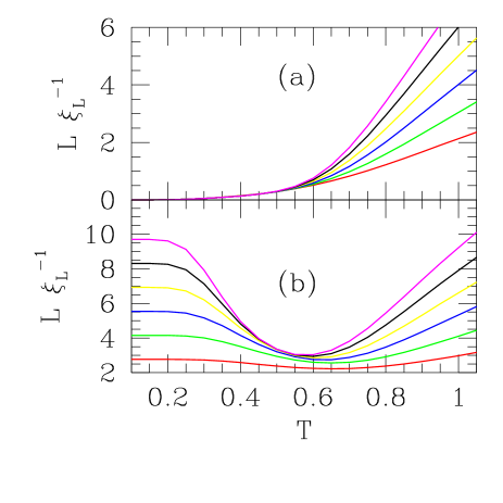
Figure 1: $L\,\xi_{L}^{-1}$ against temperature: (a) TM in the ferromagnetic direction; (b) TM in the antiferromagnetic direction. Bottom to top: $L=4,6,\dots 14$.

The raw data for $L\,\xi_{L}^{-1}$ against temperature are shown in Fig. 1, respectively (a) for the TM taken in the ferro– (F) and (b) antiferromagnetic (AF) directions. In the latter case, curves for consecutive strip widths get almost tangent as $L$ grows, in the region $T\sim 0.5-0.6$ (the $L=12$ and $14$ curves reach within one part in $10^{3}$ of each other, at $T=0.5$) . A clearer understanding of both sets of data can be gained as follows.

For the case of Fig. 1 (a) we plot the ratio of scaled mass gaps [9, 18, 22, 23, 24]

$${\cal Q}_{L\,L^{\prime}}(T)\equiv~{}\left[\,L\,\xi_{L}^{-1}(T)\,\right]/\left[\,L^{\prime}\,\xi_{L^{\prime}}^{-1}(T)\,\right]\ ,\qquad{\rm(F)}$$ (3)

where we always take $L^{\prime}=L+2$. At the fixed point of equation (2), ${\cal Q}_{L\,L^{\prime}}(T^{\ast})=1$, and one expects it to remain close to this value for an extended temperature interval if a critical phase is present [9, 18, 22, 23, 24]. Indeed this is what happens here, as shown in Fig. 2. Starting slightly below the respective $T^{\ast}$, and down to the lowest temperatures reached before running into numerical problems (typically $T=0.03-0.04$), the curves remain rather flat. The values of ${\cal Q}_{L\,L^{\prime}}$ at which they stabilize are, respectively, $1.04724$, $1.01596$, $1.00730$, $1.00394$, $1.00239$, for $L=4,6,\dots 12$. This sequence behaves as ${\cal Q}_{L\,L^{\prime}}=a+b\,L^{-x}$, where $x\simeq 2.7$ and $a$ equals unity within one part in $10^{3}$. As regards the extent of the flat region in the thermodynamic limit, the shape of curves in Fig. 2 suggests that the upper limit $T_{c}$ be given by extrapolation of the sequence of fixed points of equation (2): $T_{c}=\lim_{L\to\infty}T^{\ast}_{L\,L^{\prime}}$. Such sequence is the same given in Table 1 of [17], with the additional point $T^{\ast}_{12,14}=0.40030$. Using $L=4,6,\dots 12$ we get $T^{\ast}_{L\,L^{\prime}}=T_{c}+c\,L^{-y}$ with $T_{c}=0.29\pm 0.01$ (to be compared with $T_{c}=0.32\pm 0.03$ [17]), $y\simeq 0.7$. Thus we have convincing evidence that the system exhibits a critical phase, which extends down from $T_{c}\simeq 0.3$, at least to the lowest temperatures examined, and presumably all the way down to $T=0$.

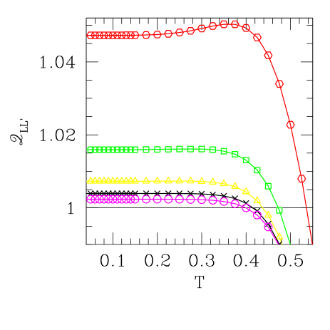
Figure 2: ${\cal Q}_{L\,L^{\prime}}(T)$ of equation (3) against $T$, for $L^{\prime}=L+2$. Top to bottom: $L=4,6,\dots 12$

In order to check on this latter assumption, it is instructive to look at the low-temperature behaviour of the correlation lengths themselves. This is illustrated in curve (a) of Fig. 3 which shows that, immediately below $T_{c}$ the functional form $\xi^{-1}=F(L)\,\exp(-1/T)$ (with $F(L)\sim L^{-1}$, from the results for ${\cal Q}_{L\,L^{\prime}}(T)$ above) sets in along the F direction. This corresponds to the lowest-energy ($T\sim 0$) excitations in that direction, which are obtained by breaking a single ferromagnetic bond, eg $\dots 000000\dots\to\dots 000111\dots$ (while, in this example, both neighbouring chains are $\dots 222222\dots$). See below the contrasting case for the AF direction. In other words, $T\to 0$ behaviour is dominant all the way down from $T_{c}$, consistent with the idea that there is a single (critical) phase from $T=0$ upwards to $T\simeq 0.3$.

Examination of data taken with the TM along the AF direction, Fig. 1 (b), is helped because the zero-temperature bulk correlation length in that direction is known exactly [12]:

$$\xi^{-1}(T=0)=\ln 2\ .\qquad{\rm(AF)}$$ (4)

We then look at the finite-temperature and finite-size deviations of $\xi^{-1}_{L}(T)$ from equation (4), as displayed in curve (b) of Fig. 3. We have been able to reach roughly the same temperatures (usually $T\sim 0.03$) as with the TM along the F direction, before running into numerical problems. The trend shown for $L=14$ in the Figure is followed for all strip widths, namely below $T\simeq 0.3$ one has

$$\ln 2-\xi^{-1}_{L}(T)=a(L)\,\exp(-2/T)\ .\qquad{\rm(AF)}$$ (5)

We have found empirically that the $L-$dependent prefactor is well fitted by a form $a(L)=a_{0}\,\exp(-b/L)$, $a_{0}\simeq 500$, $b\simeq 19.3$, except for $L=4$ which is off by $\sim 50\%$.

The factor of two in the exponential reflects the single-spin nature of elementary excitations along the AF direction, as the least costly move in this case consists in overturning a spin (breaking both its ferromagnetic bonds) without breaking any of its antiferromagnetic ones. Again, the fact that such low–$T$ behaviour takes over immediately below $T_{c}$ indicates that there is a single phase between $T=0$ and $T_{c}$.

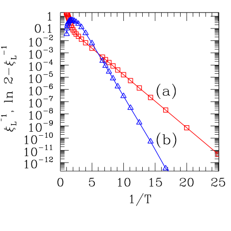
Figure 3: Curve (a): $\xi_{L}^{-1}$ against $1/T$, $L=14$, TM in the F direction. Squares are calculated points; connecting curve approaches behaviour $\sim\exp(-1/T)$ from $1/T\simeq 3$ onwards. Curve (b): $\ln 2-\xi_{L}^{-1}$ against $1/T$, $L=14$, TM in the AF direction. Triangles are calculated points; connecting curve approaches behaviour $\sim\exp(-2/T)$ from $1/T\simeq 3$ onwards.

3 Domain-wall scaling

For bulk $d-$dimensional systems, hyperscaling implies that close to the transition, the domain-wall free energy $\Delta F$ vanishes as the correlation length $\xi$ diverges, according to $\Delta F\sim\xi^{-(d-1)}$ [25]. Assuming power-law singularities, $\xi\sim|T_{c}-T|^{-\nu}$, $\Delta F\sim(T_{c}-T)^{\mu}$, $T\to T_{c}^{-}$, one has $\mu=(d-1)\nu$ [25]. Specializing to $d=2$ and using standard finite-size scaling [26], one can derive the basic fixed-point equation of domain-wall renormalisation group on strips [27]:

$$L\,\Delta f_{L}(T^{\ast})=L^{\prime}\,\Delta f_{L^{\prime}}(T^{\ast})\ ,$$ (6)

where $\Delta f_{L}$ is the free energy per unit length, in units of $T$, of a seam along the full length of the strip: $\Delta f_{L}=f^{T}_{L}-f^{P}_{L}$, with $f^{P}_{L}$ ($f^{T}_{L}$) being the corresponding free energy for a strip with periodic (twisted) boundary conditions across.

While, for Ising spins, twisted and antiferromagnetic boundary conditions coincide [27], careful consideration [28] shows that in Potts systems with $q>2$ this does not hold. Indeed, in order to produce a seam along the strip one needs an interaction which favours pairing between well-defined (and different) spin states, e.g. $1-2$, $2-3$, $3-1$. An antiferromagnetic Potts interaction only makes selected pairings energetically unfavourable, while leaving all other combinations equally probable.

Therefore, for Potts models with $q>2$, twisted boundary conditions are obtained by changing the interaction across the $L-$ direction as follows [28]:

$$J\,\delta(\sigma_{1}-\sigma_{L})\ \to J\,\delta(\sigma_{1}-\sigma_{L}+1\,({\rm mod}\ q))\ .$$ (7)

With the above definitions, one has $\Delta f_{L}=-\ln(\Lambda_{0}^{T}/\Lambda_{0}^{P})$ where $\Lambda_{0}^{T}$, $\Lambda_{0}^{P}$ are the largest eigenvalues of the TM, respectively with periodic and twisted boundary conditions across. In the present case, different results are to be expected, depending on whether the TM is set along the F or AF directions. In Figure 4 we show $L\,\Delta f_{L}$ against temperature for both cases.

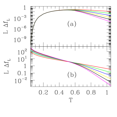
Figure 4: $L\,\Delta f_{L}$ against temperature. (a): TM in the ferromagnetic direction. On this scale, curves are indistinguishable up to $T\simeq 0.4$; top to bottom (on right-hand side): $L=4,6,\dots 14$. (b) TM in the antiferromagnetic direction. Curves cross in the central region of $T$ axis. Top to bottom (on right-hand side): $L=4,6,\dots 14$.

For case (a), the low-temperature behaviour is similar to that found in Section 2, in that all curves (i) very nearly collapse on top of each other, and (ii) behave as $\exp(-1/T)$. Analogously to the ratio of scaled mass gaps ${\cal Q}_{L\,L^{\prime}}$ used in that Section, we define the ratio of scaled free energies:

$${\cal R}_{L\,L^{\prime}}(T)\equiv~{}\left[\,L\,\Delta f_{L}(T)\,\right]/\left[\,L^{\prime}\,\Delta f_{L^{\prime}}(T)\,\right]\ ,\qquad{\rm(F)}$$ (8)

Results, using $L^{\prime}=L+2$, are displayed in Figure 5 and are very similar to those shown in Figure 2, except that instead of crossing the ${\cal R}=1$ axis from below, the curves only get asymptotically close to it, and from above. This is expected, as inverse correlation length and domain-wall free energy are dual to each other [29]. The values of ${\cal R}_{L\,L^{\prime}}$ at which the curves stabilize are, respectively, $1.03057$, $1.01029$, $1.00470$, $1.00253$, $1.00152$, for $L=4,6,\dots 12$. This sequence behaves as ${\cal R}_{L\,L^{\prime}}=e+f\,L^{-z}$, where $z\simeq 2.7$ and $e$ equals unity within two parts in $10^{4}$. Though the absence of a crossing of the ${\cal R}=1$ axis deprives one of an obvious reference point, it is possible to infer the limiting extent of the flat region, as $L\to\infty$, as follows. For each curve one records at what temperature it reaches within, say, $10^{-4}$ of its own $T\to 0$ asymptotic value, and the resulting sequence is extrapolated against $1/L$. By doing so we get $T_{c}=0.30\pm 0.04$ where the error bar, though somewhat subjective, is certainly generous enough to allow for the degree of arbitrariness involved in this procedure.

We conclude that the evidence provided is entirely consistent with that given by the analysis of correlation lengths in the F direction. As a final remark, recall that with the TM in the F direction, the seam whose energy is calculated lies parallel to ferromagnetic chains. With $q=3$, the substitution in equation (7) allows for a zero-energy seam at $T=0$, hence the behaviour depicted in Fig. 4 (a).

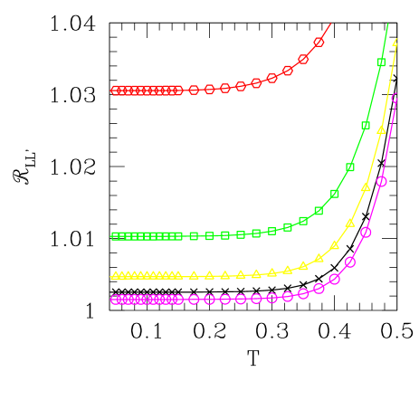
Figure 5: ${\cal R}_{L\,L^{\prime}}(T)$ of equation (8) against $T$, for $L^{\prime}=L+2$. Top to bottom: $L=4,6,\dots 12$

As regards data displayed in Figure 4 (b), one finds well-defined fixed points of equation (6). With $L^{\prime}=L+2$, these are located respectively at $T^{\ast}=0.58753$, $0.52589$, $0.48334$, $0.45108$, $0.42543$, for $L=4,6,\dots 12$. When plotted against $L^{-1}$, this sequence displays accentuated downward curvature. Attempts to fit it against $L^{-t}$ produce $t\simeq 0.1$, with a negative extrapolated value for $T_{c}$. A two-point fit of $L=10$ and $12$ data against $L^{-1}$ gives an estimate $T_{c}=0.29$. Together with the downward curvature of the full set of data, this indicates that the actual $T_{c}$ given by this particular domain-wall scaling is below $0.29$.

We recall that in the previous case with the TM along the F direction, the corresponding domain walls were found to be critical for all $0\leq T\leq T_{c}\simeq 0.30$. With the TM along the AF direction the seam runs perpendicular to that least energetic orientation of domains, breaking ferromagnetic bonds as it goes. It would thus appear that, if there is a well-defined temperature for the softening of this latter type of domain walls, it should be finite. However, we have not managed to produce a reliable estimate for this from our sequence of fixed points. Bearing in mind that the only typical non-zero temperature arising so far in the problem is $T_{c}\simeq 0.30$, one might interpret the data as signalling that the extrapolated critical point for domain walls along the AF direction is exactly $T=0$. This brings new problems, as consideration of the physical domain-wall free energy per site, $\Delta F_{L}=T\,\Delta f_{L}/L$ shows that it behaves as $1-a(L)\,T$ for $T\to 0$, with $a(L)\simeq 2.7\,\exp(-4.6/L)$. In other words, at low temperatures it becomes extremely expensive to excite a domain wall along this direction. While this behaviour is, in a loose sense, dual to that of the correlation length along the AF direction, which remains finite at $T=0$ as given by equation (4), it is hard to reconcile with the idea that the respective domain walls would go soft at $T=0$. At present we are not able to offer a consistent interpretation for the behaviour just exhibited.

4 Approach to $T_{c}$ from above: finite-size scaling

Next we attempt a characterization of the transition from the paramagnetic to the critical phase. It is usually assumed that, as this point is approached from above in a Kosterlitz-Thouless transition, the bulk correlation length behaves as [30]:

$$\xi(T)=a_{\xi}\,\exp\left[b_{\xi}\,(T-T_{c})^{-\sigma}\right]\ ,$$ (9)

with $\sigma=1/2$, and $a_{\xi}$, $b_{\xi}$ and $T_{c}$ are non-universal. From finite-size scaling [26], the correlation length on a strip is expected to scale as:

$$L\,\xi_{L}^{-1}(T)=f\left(L\,\exp\left[-b_{\xi}\,(T-T_{c})^{-\sigma}\right]\right)\ .$$ (10)

We have taken our data for correlation lengths calculated with the TM along the F direction, displayed in Fig. 1 (a) as $L\,\xi_{L}^{-1}(T)$, and attempted to fit them to the form given by equation (10). We used the procedure described in [31], to try and collapse our results for assorted values of $L$ and $T$ onto a single curve. We took as basic sets of data the six sequences taken each for fixed $L=4,6,\dots 14$ against varying temperature, from $T=0.04$ to $1.1$. According to [31], we then took each of these sets in turn as a baseline, against which to fit the five other sets. Since equation (10) is valid only above $T_{c}$, the actual number of data used would vary, for each trial fit, depending on the particular value taken for the critical temperature. With $T_{c}$ in the range $0.30-0.50$, as explained below, the number of points fitted was between $280$ ($T_{c}\simeq 0.30$) and $230$ ($T_{c}\simeq 0.50$). For the local fitting procedure [31], we used cubic polynomials.

We started by keeping $\sigma=1/2$ fixed, and varying $b_{\xi}$ and $T_{c}$. From Sections 2 and 3 $T_{c}=0.30$ would seem a reasonable initial guess. Inspired in work done on the $XY$ model [30], $b_{\xi}$ was initially assumed of order unity. The landscape we found in parameter space, for the sum of residuals [31] as a function of $b_{\xi}$ and $T_{c}$, was similar to that described in [30], with “a number of local minima … at which … minimization programs can get stuck”. Furthermore, visual inspection of plots produced with the parameters set at the minimizing values gave consistently poor fits in all cases for which $T_{c}$ was below $0.35$. We did, however, manage to find an overall minimum for $T_{c}=0.51\pm 0.01$, $b_{\xi}=1.72\pm 0.01$ (with none for $0.35\leq T_{c}\leq 0.50$).

We then allowed $\sigma$ to vary. The overall picture was entirely similar to that just described for fixed $\sigma=1/2$. The only solution which gave a visually confirmed good fit was $T_{c}=0.50\pm 0.01$, $b_{\xi}=1.60\pm 0.01$, $\sigma\simeq 0.54$. The corresponding results are shown in Fig. 6.

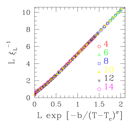
Figure 6: Scaling plot (see equation (10)) of data displayed in Fig.1 (a). The parameters are: $T_{c}=0.51$, $b_{\xi}=1.60$, $\sigma=0.54$ (see text).

The value $T_{c}\simeq 0.50$ is inconsistent with the evidence exhibited in Sections 2 and 3. One possible solution to this contradiction would be if the critical region, where the behaviour of equation (10) is valid, were actually very narrow. Thus, we would be distorting the picture, by using high-temperature data which in fact are outside the critical region. For the $XY$ model in two dimensions, it has been argued that this is indeed the case [30, 32, 33], with the width of the critical region estimated as $(T-T_{c})/T_{c}\leq 10^{-2}$ [33]. With $T_{c}\simeq 0.3$, in the present case this would mean a temperature interval $\Delta T\simeq 3\times 10^{-3}$. For the fitting shown in Fig. 6 we used data for $T$ as high as $2.5$, for the narrowest strips. We noticed that, if only a subset of data with $T\leq 1.1$ is used, the best fit is found for $T_{c}\simeq 0.47$, and is of similar quality to that of Fig. 6. Thus a plausible scenario is one in which, as only data for an ever narrowing interval above $T_{c}$ are considered, the corresponding fits give rise to lower and lower estimates of $T_{c}$ itself. Should the prediction of [33] hold true in the present case, one would have a problem in that the accuracy to which $T_{c}$ is known so far (taking, say, our best estimate $0.29\pm 0.01$ of Section 2) is lower than the width $\Delta T$ of the critical region.

5 Conclusions

We have provided strong numerical evidence that a critical (Kosterlitz-Thouless) phase is present in the three-state mixed Potts magnet described by equation (1). Our argument relies on the analysis of the quantities ${\cal Q}_{L\,L^{\prime}}(T)$ and ${\cal R}_{L\,L^{\prime}}(T)$, defined respectively in equations (3) and (8). Based on data exhibited in Figures 2 and 5 and their respective extrapolation, we conclude that the upper limit of the critical phase, above which the system behaves paramagnetically, is $T_{c}=0.29\pm 0.01$ (from Figure 2; treatment of data in Figure 5 produces the less accurate, but not inconsistent, estimate $T_{c}=0.30\pm 0.04$).

Analysis of the (extremely anisotropic) nature of excitations below $T_{c}$, as depicted in Figure 3, gives credence to the idea that the critical phase extends all the way down to $T=0$, similarly to what happens in the two-dimensional $XY$ model.

We have found that, while domain walls parallel to the ferromagnetic direction are soft for the whole extent of the critical phase, those along the antiferromagnetic direction seem to undergo a softening transition at a well-defined, finite temperature. However, from our data we have not been able to produce a reliable estimate for location of such transition.

Attempts to fit our data for $T>T_{c}$ to the finite-size scaling form of equation (10) have met with qualified success. While we have been able to produce rather good collapse plots, as depicted in Figure 6, this has been done at the price of setting $T_{c}=0.50\pm 0.01$ which is clearly inconsistent with our own earlier estimates. We have proposed a scenario in which such result is interpreted as a distortion due to the narrowness of the critical region, similarly to the case of the $XY$ model [30, 32, 33]. This is qualitatively borne out by the fact that fits with only a subset of data, taken at not too high temperatures, indeed result in a lower estimate for $T_{c}$.

References

References

- [1] Kosterlitz J M and Thouless D J 1973 J. Phys. C: Solid State Phys.6 1181
- [2] José J V, Kadanoff L P, Kirkpatrick S and Nelson D R 1977 Phys. Rev.B 16 1217
- [3] Elitzur S, Pearson R B and Shigemitsu J 1979 Phys. Rev.D 19 3698
- [4] Nienhuis B, Hilhorst H J and Blöte H W J 1984 J. Phys. A: Math. Gen.17 3559
- [5] Blöte H W J, Nightingale M P, Wu X N and Hoogland A 1991 Phys. Rev.B 43 8751
- [6] Blöte H W J and Nightingale M P 1993 Phys. Rev.B 47 15 046
- [7] Domany E, Schick M, Walker J S and Griffiths RB 1978 Phys. Rev.B 18 2209
- [8] Landau D P 1983 Phys. Rev.B 27 5604
- [9] de Queiroz S L A and Domany E 1995 Phys. Rev.E 52 4768
- [10] Wu F Y 1982 Rev. Mod. Phys.54 235
- [11] Ostlund S 1981 Phys. Rev.B 24 398
- [12] Kinzel W, Selke W and Wu F Y 1981 J. Phys. A: Math. Gen.14 L399
- [13] Herrmann H J and Mártin H O 1984 J. Phys. A: Math. Gen.14 657
- [14] Truong T T 1984 J. Phys. A: Math. Gen.17 L473
- [15] Selke W and Wu F Y 1987 J. Phys. A: Math. Gen.20 703
- [16] Yasumura K 1987 J. Phys. A: Math. Gen.20 4975
- [17] Foster D P and Gérard C 2002 J. Phys. A: Math. Gen.35 L75
- [18] Roomany H H and Wyld H W 1980 Phys. Rev.D 21 3341
- [19] Nightingale M P and Schick M 1982 J. Phys. A: Math. Gen.15 L39
- [20] Derrida B and de Seze L 1982 J. Physique43 475
- [21] Houlrik J M, Knak Jensen S J and Bak P 1983 Phys. Rev.B 28 2883
- [22] Hamer CJ and Barber MN 1981 J. Phys. A: Math. Gen.14 259
- [23] Schaub B and Domany E 1983 Phys. Rev.B 28 2897
- [24] Domany E and Schaub B 1984 Phys. Rev.B 29 4095
- [25] Watson P G 1972 Phase Transitions and Critical Phenomena Vol 2, ed C Domb and M S Green (London: Academic) p 101
- [26] Barber M N 1983 Phase Transitions and Critical Phenomena Vol 8, ed C Domb and J L Lebowitz (London: Academic) p 145
- [27] McMillan W M 1984 Phys. Rev.B 29 4026
- [28] Park H and den Nijs M 1988 Phys. Rev.B 38 565
- [29] Cardy J L 1984 J. Phys. A: Math. Gen.17 L961
- [30] Gupta R and Baillie C F 1992 Phys. Rev.B 45 2883
- [31] Bhattacharjee S M and Seno F 2001 J. Phys. A: Math. Gen.34 6375
- [32] Greif J M, Goodstein D L and Silva-Moreira A F 1982 Phys. Rev.B 25 6838
- [33] Cardy J L 1982 Phys. Rev.B 26 6311