[

Effective action and interaction energy of coupled quantum dots

Abstract

We obtain the effective action of tunnel-coupled quantum dots, by modeling the system as a Luttinger liquid with multiple barriers. For a double dot system, we find that the resonance conditions for perfect conductance form a hexagon in the plane of the two gate voltages controlling the density of electrons in each dot. We also explicitly obtain the functional dependence of the interaction energy and peak-splitting on the gate voltage controlling tunneling between the dots and their charging energies. Our results are in good agreement with recent experimental results, from which we obtain the Luttinger interaction parameter $K=0.74$.

]

Coulomb blockade CB[2] in quantum dots has gained in importance in recent years, due to its potential for application as single electron transistors. Recent experiments[3, 4, 5] on coupled quantum dots have revealed a variety of features, the most salient of which is the conductance peak splitting controlled by inter-dot tunneling. The peaks split into two for a double dot system and into three for a triple dot system.

Earlier theoretical studies[6] on coupled dots studied the effect of tunneling and inter-dot capacitances on the CB, but only a few[7, 8, 9] focused on junctions with only one or two channels. Motivated by a) the double dot experiments, b) the analysis of Matveev[10], which maps a quantum dot formed by a narrow constriction that allows only one transverse channel to enter the dot, to a one-dimensional wire model and c) recent numerical evidence[11] that justifies modeling of quantum dots by Luttinger liquids, we model the coupled dot system as a one-dimensional Luttinger liquid (LL) with large barriers and study the effective action in the coherent limit.

We obtain a simple expression for the interaction energy in terms of the charging energies of the two dots and the gate voltage controlling the inter-dot tunneling, and find that tunneling between the dots splits the conductance maxima. With (without) inter-dot tunneling, the conductance (resonance) maxima, for a double dot system, form a rectangular (hexagonal) grid in the plane of the two gate voltages controlling the density of the electrons. The peak splitting grows to a maximum when the two dots merge into a single dot. From the experiments, we estimate the interaction energy and also the values for the Luttinger parameters.

Although a classical analysis with an inter-dot capacitance reproduces the experimental results qualitatively, the value of the required inter-dot capacitance is unrealistically large[3]. Golden and Halperin[8] obtain their results by mapping the two dot model to a single dot model. Here, we directly model the experimental set-up as a one-dimensional system and obtain the effective action exactly, by integrating out Gaussian degrees of freedom. Hence our results give the interaction energy directly in terms of the microscopic variables and applied voltages. We find that in the weak tunneling limit, the peak splitting is proportional to the square-root of the tunneling conductance and in the strong tunneling limit, the deviation of the splitting factor from unity is proportional to the square-root of the deviation of the conductance (measured in units of $2e^{2}/h$) from unity.

Model and effective action for coupled quantum dots

Our model for a dot is essentially a short length of LL wire with barriers at either end, controlling the tunneling to and from the dot. The two dot system is shown in Fig.(1), with three barriers in the LL wire between the two leads. The barriers are chosen to be $\delta$-functions with strengths $G_{i}$ and $J$. (Extended barriers do not change the results[8].) The electrons in the dot interact via a short range (Coulomb-like) interaction described by the Hamiltonian $H=-v_{F}\int dx[\psi_{L}^{\dagger}i\partial_{x}\psi_{L}-(L\leftrightarrow R)]+g\int dx\rho(x)^{2}$ where $\rho(x)=\psi^{\dagger}\psi$ is the electron density and $\psi=\psi_{L}e^{-ik_{F}x}+\psi_{R}e^{ik_{F}x}$. Here, $\psi_{R}$ and $\psi_{L}$ stands for fermion fields linearised about the left and right Fermi points. The electrons in the leads are free.

The model is bosonised via the standard transformation $\psi_{\nu}=\eta_{\nu}e^{2i\sqrt{\pi}\phi_{\nu}}$ where $\nu=R,L$ and $\phi_{\nu}$ are the bosonic fields. $\eta_{\nu}$ are the Klein factors that ensure anti-commutation of the fermion fields. The Lagrangian density for the bosonic field in 1+1 dimensions is ${\cal L}(\phi;K,v)=(1/2Kv)(\partial_{t}\phi)^{2}-(v/2K)(\partial_{x}\phi(x))^{2}$, where $K\sim(1+g/\pi v_{F})^{-1/2}$ and $v\sim v_{F}(1+g/\pi v_{F})^{1/2}$. The bosonised action is now given by[12, 13, 14]

$$S=\int d\tau[S_{leads}+S_{dots}+S_{gates}]~{},$$ (1)

with $S_{leads}=(\int_{-\infty}^{-d_{1}}+\int_{d_{2}}^{\infty})dx{\cal L}(\phi;K_{L}=1,v_{F})$, $S_{dots}=\int_{-d_{1}}^{0}dx{\cal L}(\phi;K_{1},v_{1})+\int_{0}^{d_{2}}dx{\cal L}(\phi;K_{2},v_{2})+V+J\cos(2\sqrt{\pi}\chi)$ and $S_{gates}=(g_{1}/\sqrt{\pi})\int_{-d_{1}}^{0}dx(\chi-\phi_{1})+(g_{2}/\sqrt{\pi})\int_{0}^{d_{2}}dx(\phi_{2}-\chi)~{}$, where $V=\Sigma_{i=1}^{2}G_{i}\cos(2\sqrt{\pi}\phi_{i}+(-1)^{i}2k_{F}d_{i})$. Here $G_{i}$ and $J$ are the junction barriers defining the dots and $\phi_{i}\equiv\phi((-1)^{i}d_{i})$ and $\chi\equiv\phi(0)$ denote the boson fields at those points. $J$ controls tunneling between the dots and ranges from fully open ($J=0$, single dot ) to fully closed ($J=\infty$, two decoupled dots). The gate voltages $g_{i}$ control the density of electrons in each dot.

FIG. 1.: Double dot system above shown schematically below with the dots modeled as LL with $K_{i=1,2}$, between barriers $G_{i}$ and $J$, and with two gate voltages $g_{i}$.

In the low $T$ limit ($T\ll\hbar v_{1}/k_{B}d_{1},\hbar v_{2}/k_{B}d_{2}$) all three barriers are seen coherently, and we expect the CB of the two dots to be coupled. The effective action of the system can be obtained by integrating out all degrees of freedom except those at the positions of the three junction barriers, following Ref. [12, 13] and we find that

$$S_{ef} = S_{0}+\int d\tau\{\Sigma_{i=1}^{2}[{U_{i}\over 2}(\chi-\phi_{i})^{2}+(-1)^{i}{g_{i}\over\sqrt{\pi}}(\chi-\phi_{i})]$$ (3)

$$+V+J\cos{(2\sqrt{\pi}\chi)}\}$$

where $S_{0}=\sum_{\omega_{n}}|\omega_{n}|({\tilde{\phi}}_{1}^{2}+{\tilde{\phi}}_{2}^{2})/2(K_{L}=1)$ . The Fourier transformed tilde fields are defined by $\phi_{i}(\tau)=\sum_{\omega_{n}}e^{-i\omega_{n}\tau}{\tilde{\phi}}_{i}(\omega_{n})$. The $U_{i}=\hbar v_{i}/K_{i}d_{i}$ terms are the ‘mass’ terms that suppress charge fluctuations on the dots and are responsible for the CB through the dots.

Weak tunneling limit

Here the barrier $J$ is very large, and the field $\chi$ is pinned at its minima -

$$\chi=n\sqrt{\pi}\equiv\chi_{cl}\quad(n={\rm integer}).$$ (4)

A semi-classical expansion about these minima using $\chi=\chi_{cl}+\chi_{q}$ to second order in the fluctuations yields

$$S_{ef} \simeq S_{0}+\int d\tau\{[-g_{1}\phi_{1}+g_{2}\phi_{2}]/\sqrt{\pi}~{}+~{}\chi_{q}(g_{1}-g_{2})/\sqrt{\pi}$$ (7)

$$+\Sigma_{i=1}^{2}{U_{i}}\big{[}\chi_{q}^{2}+2\chi_{q}(\chi_{cl}-\phi_{i})+(\chi_{cl}-\phi_{i})^{2}\big{]}/2$$

$$+V-(2\pi J)\chi_{q}^{2}\}$$

where we have dropped all field-independent constants. We can now integrate out the quantum fluctuations in $\chi$, since we have only kept quadratic terms, and using $J\gg U_{i},g_{i}$, we get

$$S_{ef} \simeq S_{0}+\int d\tau[\Sigma_{i=1}^{2}{U_{i}\over 2}(\chi_{cl}-\phi_{i})^{2}+{U_{1}U_{2}\over 4\pi J}\phi_{1}\phi_{2}$$ (9)

$$+{(-g_{1}\phi_{1}+g_{2}\phi_{2})/\sqrt{\pi}}+V]~{}.$$

Now, we define the following variables - $n_{i}=(-1)^{i+1}(\chi_{cl}-\phi_{i})/\sqrt{\pi}+(k_{F}d_{i})/\pi$ and $\theta_{i}=(\chi_{cl}+\phi_{i})/2+(-1)^{i}(k_{F}d_{i})/2$ which can be interpreted as the charges and currents on the dots 1 and 2 respectively and in terms of which the action can be rewritten simply as

$$S_{ef} \simeq S_{0} +\int d\tau[\Sigma_{i=1}^{2}{{\cal U}_{i}\over 2}(n_{i}-n_{0i})^{2}-E_{12}n_{1}n_{2}+V]$$ (10)

$${\rm where}$$ (11)

$$E_{12} = {U_{1}U_{2}/4J},~{}~{}\&~{}~{}n_{0i}=(k_{F}d_{i})/\pi-g_{i}/{\cal U}_{i}~{}.$$ (12)

${\cal U}_{i}\equiv\pi U_{i}$ plays the role of the charging energy or CB energy because in the absence of any mixing between $n_{1}$ and $n_{2}$, by tuning $g_{i}$ (equivalently $n_{0i}$), the dot states with $n_{i}$ and $n_{i}+1$ electrons can be made degenerate. This is the lifting of the CB for each individual dot. But the crucial term above is the term mixing $n_{1}$ and $n_{2}$. This tells us how the CB through one dot is affected by the charge on the other dot. The barrier terms can be more conveniently rewritten in terms of the total charge of the double dot and the current through the double dot system, when $G_{1}=G_{2}=G$ by defining the total charge and current fields as $N=n_{1}+n_{2}=(\phi_{2}-\phi_{1})/\sqrt{\pi}+({k_{F}L})/\pi$ and $\theta=(\phi_{2}+\phi_{1})/2+({k_{F}l})/2\sqrt{\pi}$, where $L=d_{1}+d_{2}$ and $l=d_{2}-d_{1}$. With these redefinitions, the barrier term reduces to

$$V=2G\cos(2\sqrt{\pi}\theta)\cos\pi N~{},$$ (13)

and $S_{0}\rightarrow S^{\prime}_{0}=\sum_{\omega_{n}}|\omega_{n}|({\tilde{\theta}}^{2}+(\pi/4){\tilde{N}}^{2})$. The action is now in a form where its symmetries are manifest.

When the two dots are decoupled from each other ($E_{12}=0$ or equivalently $J\rightarrow\infty$), the action is symmetric under the transformation $\theta\rightarrow\theta+\sqrt{\pi},~{}~{}N\rightarrow 2N_{0}-N$. This is because $g_{1}$ and $g_{2}$ can be tuned so as to make $n_{01},n_{02}$ to be half-integers $q_{1}+1/2,q_{2}+1/2$ and hence, $N_{0}=n_{01}+n_{02}$ to be an integer. Thus the two CB’s are lifted and the four charge states, $(n_{1},n_{2})=(q_{1},q_{2}),(q_{1}+1,q_{2}),(q_{1},q_{2}+1)(q_{1}+1,q_{2}+1)$ become degenerate and transport through the double dot system is unhindered. We can plot the points of maximum conductance through the double-dot system in the plane of the two gate voltages and as shown by the dotted lines in Fig.(2), we get a square grid. (The figure is for identical dots; in general, the grid is rectangular.)

FIG. 2.: Positions of the conductance maxima as a function of the gate voltages. The solid lines denote the splitting and the dot-dash line AB denotes the distance between two sets of split peaks. The splitting factor $S$ is defined as twice the ratio of the former to the latter length.

Now, we study the symmetries for a large finite $J$. In this case, the CB through each dot is influenced by interaction with the electrons in the other dot. Hence, we now find that the CB through the double dot system is lifted for two possible sets of gate voltages -
$\bullet$ the states [$(q_{1},q_{2})$, $(q_{1}+1,q_{2})$] and the states [$(q_{1},q_{2})$, $(q_{1},q_{2}+1)$] are degenerate simultaneously respectively when

$$n_{01}=q_{1}+{1\over 2}+{U_{2}\over 8J}q_{2},~{}~{}~{}n_{02}=q_{2}+{1\over 2}+{U_{1}\over 8J}q_{1}$$ (14)

This is one point where the CB is lifted and the conductance is a maximum.
$\bullet$ Similarly, the states [$(q_{1},q_{2}+1)$, $(q_{1}+1,q_{2}+1)$] and [$(q_{1}+1,q_{2})$, $(q_{1}+1,q_{2}+1)$] are degenerate simultaneously when

$$n_{01}=q_{1}+{1\over 2}+{U_{2}\over 8J}(q_{2}+1),~{}~{}~{}n_{02}=q_{2}+{1\over 2}+{U_{1}\over 8J}(q_{1}+1)$$ (15)

This is another point where the CB is lifted and the conductance is a maximum.
Note that the original resonance which occured when all four states were degenerate has now broken into two separate resonances, at each of which only three states are degenerate. Plotting this in the plane of the gate voltages, we obtain a hexagon as shown by the dashed and solid lines in Fig.(2) in agreement with the experiments of Blick et al in [4]. (The figure shown is for identical dots; otherwise, the hexagons are not perfectly symmetric.) Thus, as a consequence of tunneling between the quantum dots, the conductance maxima splits into two.

The splitting $\delta g$ of the maxima as a function of the tunneling barrier $J$ (the solid line in Fig.(2)) can be computed from Eqs(14) and (15), and gives

$$\delta g_{1}=\delta g_{2}=\pi U_{1}U_{2}/8J~{}\Rightarrow\delta g={\sqrt{2}}\pi U_{1}U_{2}/8J~{}.$$ (16)

Hence, the splitting in $g_{1}$ and $g_{2}$ is identical and is inversely proportional to the gate voltage controlling the tunneling barrier and directly proportional to the charging energies of the two dots. However, when $J$ becomes comparable to the other energy scales in the problem like $U_{i}$, the strong barrier analysis breaks down.

Strong tunneling or weak barrier limit

Here we assume that the barrier between the two dots is very small - $i.e.$, $G_{i}\gg U_{i}\gg J$. So essentially, there is only one CB. However, we shall see that the spacing of the CB terms are affected by a non-zero $J$. We integrate out $\chi$ (in Eq.3) which is quadratic (when $J$ is ignored) to obtain

$$S_{ef} = \Sigma_{\omega_{n}}|\omega_{n}|({\tilde{\theta}}^{2}+{\pi\over 4}{\tilde{N}}^{2})+U_{ef}(N-N_{0})^{2}/2$$ (17)

$$+ 2G\cos(2\sqrt{\pi}\theta)\cos\pi N+J\cos[2\sqrt{\pi}\theta+X\pi N+C]~{}$$ (18)

$$= S_{0}+V_{ef}~{}.$$ (19)

Here, we have defined $U_{ef}=\pi U_{1}U_{2}/(U_{1}+U_{2})=\pi U/2$, $X=(U_{1}-U_{2})/(U_{1}+U_{2})=0$, $N_{0}=k_{F}L/\pi-(g_{1}/{\cal U}_{1}+g_{2}/{\cal U}_{2})=k_{F}L/\pi-g/U_{ef}$, $C=2(g_{2}-g_{1})/(U_{1}+U_{2})+(U_{1}+U_{2})k_{F}l+(U_{1}-U_{2})k_{F}L=0$. $N$ and $\theta$ have been defined earlier. $C$ and $N_{0}$ depend on the gate voltages and are the tunable parameters. The second equalities are for identical dots when $U_{1}=U_{2}=U$ and $d_{1}=d_{2}$. $g_{1}=g_{2}=g$ can be tuned by $C$. We shall use these values below for simplicity.

Since, we continue to be in the strong barrier limit for the $G$ term, the action has deep minima for integer $N$ (with appropriate $\theta$). But the degeneracy between these minima is broken by the $U_{ef}$ and $J$ terms leading to just one of them being preferred (as is the case for the usual CB without $J$). Just as earlier, the CB is lifted when

$$V_{ef}(\theta,N)=V_{ef}(\theta+\sqrt{\pi}/2,N+1)~{}.$$ (20)

When $J=0$, this happens when $N_{0}=$ half-integer. However, when $J\neq 0$, the above equality holds when

$$N_{0}={1/2}-{J/U_{ef}},{3/2}+{J/U_{ef}},{5/2}-{J/U_{ef}}\dots,$$ (21)

which implies that the splitting $\delta g$ is given by

$$\delta g=U_{ef}-2J~{}.$$ (22)

It is easy to see from Eq.(21) that periodicity is restored when two electrons are added to the system, but periodicity when a single electron is added to the system is broken by the $J$ term. This tells us that the main effect of a small barrier within a single dot, is to change the spacing of the peaks with two peaks coming closer to each other and pairs of peaks receding from each other. But the distance between pairs of peaks remains $2U$. As $J$ increases towards $\infty$, the peaks which come closer to one another slowly merge into one, and we are left with half as many peaks, which is what one would expect when the dot size is halved.

Discussions and conclusions

Thus, both from the weak and strong tunneling limits, we get a consistent picture. The splitting is zero for $J=\infty$ and maximum when the tunneling goes to one ($J=0$) and is just the spacing of a single dot of length $d_{1}+d_{2}$. As a function of the tunneling barrier, the splitting saturates linearly (proportional to $J$) for low barriers (strong tunneling) and goes as $1/J$ for weak tunneling (strong barriers). (Our model does not include inter-dot capacitance since it is expected to be very small for the experiment[3].) In terms of the barrier conductance $G_{b}$, simple quantum mechanics shows that $G_{b}$ (in units of $2e^{2}/h$) falls off from unity as $J^{2}$ in the low barrier limit and increases from zero as $1/J^{2}$ in the weak tunneling limit. So in the weak tunneling limit, using Eq.(16) and Fig. 2, the splitting factor $S=\delta g/(U+\delta g)\sim\delta g/U$ (for $\delta g\ll U$) $\propto 1/J\propto\sqrt{G}_{b}$. In the strong tunneling limit, $S=2\delta g/2U_{ef}=1-2J/U_{ef}$. So $1-S\propto J\propto\sqrt{1-G_{b}}$ Thus, in both limits, we relate the splitting factor to the barrier conductance. This is the central result of this letter.

In Fig.3, we compare our theoretical prediction of $S$ with the experimental curve. In the weak tunneling limit, a one-parameter $\chi^{2}$ fit of our prediction to the lowest five points (upto $S\sim 0.3$) gives a goodness of fit of 84% . In contrast, a linear fit to the same data ( predicted in Ref.[8]), gives a goodness of fit of only 75%. Similarly, in the strong tunneling limit ($S$ above $0.7$), a one parameter fit of our prediction (which, in fact, is in agreement with the scaling analysis of Ref.[15]) gives a goodness of fit of 96%, again, considerably better than the 81% for the logarithmic prediction in Ref.[8]. However, although our modelling is more realistic than earlier ones and the agreement of our predictions with the experimental data, both in the strong and weak tunneling limits is impressive, better data is required for a conclusive proof. Further, we predict that for the weak tunneling case, the interdot interaction energy is directly proportional to the charging energies of the dots and hence inversely proportional to the sizes or capacitances of each of the individual dots.

The charging energies and the Fermi velocity obtained from Ref.[3] are $U_{i}\sim 400\mu eV$. and $(v_{F})_{1d}\sim 2.3\times 10^{7}cm$. Thus using the relation, $U=\hbar v/Kd$, for a single dot, we find the LL parameters, $v_{1}=v_{2}\sim 3.1\times 10^{7}cm/sec$ and $K_{1}=K_{2}\sim.74$ for identical dots. In the weak barrier limit, where the splitting is small, we find that $E_{12}$ (in Eq.12) ranges from $\sim 4-40\mu eV$, which is roughly $(10^{-2}-10^{-1})U$. The LL parameter values remain almost unchanged in the range of gate voltages used in the experiments. The values can be confirmed by studying the conductance through the double dot system in the ‘high’ temperature limit, $T\gg T_{d}=\hbar v/k_{B}d\sim 0.6K$, when the electron transport through each of the dots is incoherent. The conductance should scale as $T^{2(1/K-1)}\sim T^{0.69}$ in the weak tunneling case and as $T^{2(K-1)}\sim T^{-0.51}$ in the weak barrier case. LL behaviour can also be probed if the conductances are studied as a function of the size of the dots at ‘low’ temperatures $T\ll T_{d}$ since LL theory predicts explicit size dependent power laws at low temperatures.

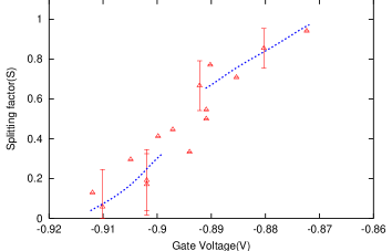
FIG. 3.: Splitting factor $S$ as function of the gate voltage controlling tunneling. The data points are from Ref.(2). The solid line denotes the square-root of the measured conductance (multiplied by scaling factor 0.56 for best fit), and the dotted line just denotes the measured conductance (multiplied by 0.60 for best fit).

In conclusion, in this letter, we have obtained the effective action of a system of coupled quantum dots, in both the weak and strong tunneling limits. We have shown that in the presence of inter-dot tunneling, the peaks denoting the conductance maxima split. The split is maximum when the tunneling between the dots is maximum - i.e., when there is no barrier at all between the dots. We have also computed the splitting as a function of the gate voltage controlling the tunneling between the dots in both the weak and strong tunneling limits, and find that the splitting factor is proportional to the square-root of the conductance in the weak tunneling limit and the deviation of the splitting from unity is proportional to the square-root of the deviation of the conductance from unity in the strong tunneling limit. This agrees with the experimental data on double dot systems. We have also extracted the Luttinger parameters from the experiment and have predicted temperature power laws for the same set-up which can be experimentally tested.

REFERENCES

- [1]
- [2] Single charge tunneling, edited by H. Grabert and M. H. Devoret, ( Plenum Press, New York, 1992)
- [3] F. R. Waugh et al, Phys. Rev. Lett.75, 705 (1995); F. R. Waugh et al, Phys. Rev. B53, 1413 (1996).
- [4] Molenkamp et al, Phys. Rev. Lett.75, 4282 (1995); van der Vaart et al Phys. Rev. Lett.74, 4702; R. H. Blick et al, Phys. Rev. B53, 7899 ((1996); D. C. Dixon et al, Phys. Rev. B53, 12625 (1996); C. Livermore et al, Science 274, 1332 (1996); Fujisawa et al, Science 282, 932 (1998).
- [5] For a review, see W. G. van der Wiel et al, cond-mat/0205350.
- [6] I. M. Ruzin et al, Phys. Rev. B45, 13469 (1992); L. I. Glazman and V. Chandrasekhar, Europhys. Lett. 19, 623 (1992); C. A. Stafford and S. Das Sarma, Phys. Rev. Lett.72, 3590 (1994); G. Klimeck, G. Chen and S. Datta, Phys. Rev. B50, 2316 (1994).
- [7] K. A. Matveev, L. I. Glazman and H. U. Baranger, Phys. Rev. B53, 1034 (1996); ibid 54 5637 (1996).
- [8] J. M. Golden and B. I. Halperin, Phys. Rev. B53, 3893 (1996); ibid 65, 115326 (2002).
- [9] S. Lamba and S. K. Joshi, Phys. Rev. B62, 1580 (2000).
- [10] K.A.Matveev, Phys. Rev. B51, 1743 (1995).
- [11] P. Rojt, Y. Meir and A. Auerbach, Phys. Rev. Lett.89, 256401 (2002).
- [12] C. L. Kane and M. P. A. Fisher, Phys. Rev. B 46, 15233 (1992).
- [13] S. Lal, S. Rao and D. Sen, Phys. Rev. Lett. 87, 026801 (2001); ibid Phys. Rev. B 65, 195304 (2002).
- [14] For a review, see S. Rao and D. Sen, cond-mat/005492, published in ‘Field theories in condensed matter physics, Ed. S. Rao, (IOP publications, U.K., May 2002).
- [15] K. Flensberg, Phys. Rev. B 48, 11156 (1993).