1 Introduction

Dynamic fluctuation properties of mesoscopic electrical conductors provide additional information not obtainable through conductance measurement. Indeed, over the last decade, experimental and theoretical investigations of current fluctuations have successfully developed into an important subfield of mesoscopic physics. A detailed report of this development is presented in the review by Blanter and Büttiker [1].

In this work we are concerned with the correlation of current fluctuations which can be measured at different terminals of multiprobe conductors. Of particular interest are situations where, as a function of an externally controlled parameter, the sign of the correlation function can be reversed.

Electrical correlations can be viewed as the Fermionic analog of the Bosonic intensity-intensity correlations measured in optical experiments. In a famous astronomical experiment Hanbury Brown and Twiss demonstrated that intensity-intensity correlations of the light of a star can be used to determine its diameter [2]. In subsequent laboratory experiments of light split by a half-silvered mirror statistical properties of light were further analyzed [3]. Much of modern optics derives its power from the analysis of correlations of entangled optical photon pairs generated by non-linear down conversion [4]. The intensity-intensity correlations of a thermal Bosonic source are positive due to statistical bunching. In contrast, anti-bunching of a Fermionic system leads to negative correlations [5].

Concern with current-current correlations in mesoscopic conductors originated with Refs. [6, 7]. The aim of this work was to investigate the fluctuations and correlations for an arbitrary multiprobe conductor for which the conductance matrix can be expressed with the help of the scattering matrix [8, 9]. Refs. [6, 7] provided an extension of the discussions of shot noise by Khlus [10] and Lesovik [11] which applies to two-terminal conductors. These authors assumed from the outset that the transmission matrix is diagonal and provided expressions for the two terminal shot noise in terms of transmission probabilities. It turns out that even for two probe conductors, shot noise can be expressed in terms of transmission probabilities only in a special basis (eigen channels). Such a special basis does not exist for multiprobe conductors and we are necessarily left with expressions for shot noise in terms of quartic products of scattering matrices [7, 12]. There are exceptions to this rule: for instance correlations in three-terminal one-channel conductors can also be expressed in terms of transmission probabilities only [13].

The reason that shot noise, in contrast to conductance, is in general not simply determined by transmission probabilities is the following: if carriers incident from different reservoirs (contacts) or quantum channels can be scattered into the same final reservoir or quantum channel, quantum mechanics demands that we treat these particles as indistinguishable. We are not allowed to be able to distinguish from which initial contact or quantum channel a carrier has arrived. The noise expressions must be invariant under the exchange of the initial channels [14, 15, 16, 17, 18]. The occurrence of exchange terms is what permitted Hanbury Brown and Twiss to measure the diameter of the stars: Light emitted by widely separated portions of the star nevertheless exhibits (a second order) interference effect in intensity-intensity correlations [2].

Experiments which investigate current-correlations in mesoscopic conductors have come along only recently. Oliver et al. used a geometry in which a ”half-silvered mirror” is implemented with the help of a gate that creates a partially transparent barrier [19]. Henny et al. [20] separated transmission and reflection along edge states of a quantum point contact subject to a high magnetic field. In the zero temperature limit an electron reservoir compactly fills all the states incident on the conductor. A subsequent experiment by Oberholzer at al. [21] uses a configuration with two quantum point contacts, as shown in Fig. 1. This geometry permits to thin out the occupation in the incident electron beam and thus allows to investigate the transition in the correlation as we pass from degenerate Fermi statistics to dilute Maxwell-Boltzmann satistics. Anti-bunching effects vanish in the Maxwell-Boltzmann limit and the current-current correlation tends to zero as the occupation of the incident beam is diminished. The fact that in electrical conductors the incident beam is highly degenerate is what made these Hanbury Brown Twiss experiments possible. In contrast, an emission of electrons into the vacuum generates an electron beam with only a feeble occupation of electrons [22] and for this reason an experiment in vacuum has in fact just been achieved only very recently [23]. Below we will discuss the experiments in electrical conductors in more detail.

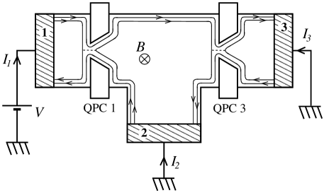
Figure 1.  : Experimental arrangement of Oberholzer at al. Current is injected at contact $1$. One edge channel is perfectly transmitted (and noiseless) the other is partially transmitted at QPC 1 with probability $T_{1}$ and partially transmitted at QPC 3 with probability $T_{3}$ into contact $3$ and reflected with probability $R_{3}=1-T_{3}$ into contact $2$. Of interest is the correlation of currents measured at contacts $2$ and $3$.

Within the scattering approach, in the white noise limit, it can be demonstrated, that current-current correlations are negative, irrespective of the voltages applied to the conductor, temperature and geometry of the conductor [7, 12]. The wide applicability of this statement might give the impression, that in systems of Fermions current correlations are always negative. However, the proof rests on a number of assumptions: in addition to the white-noise limit (low frequency limit) it is assumed that the terminals are all held at a constant (time-independent) terminal-specific potential. This is possible if the mesoscopic conductor is embedded in a zero-impedance external circuit. No general statement on the sign of correlations exists if the external circuit is characterized by an arbitrary impedance.

In this work we are interested in situations for which the above mentioned proof does not apply. For instance, a voltmeter ideally has infinite impedance, and a conductor in which one of the contacts is connected to a voltmeter presents a simple example in which it is possible to measure positive current-current correlations [24]. In steady state transport the potential at a voltage probe floats to achieve zero net current. If the currents fluctuate the potential at the voltage probe must exhibit voltage fluctuations to maintain zero current at every instant. As has been shown by Texier and Büttiker, the fluctuating potential at a voltage probe can lead to a change in sign of a current-current correlation [24].

A voltage probe also relaxes the energy of carriers, it is a source of dissipation [25, 26, 27, 28]. Probes which are non-dissipative are of interest as models of dephasors. At low temperatures dephasing is quasi-elastic and it is therefore reasonable to model dephasing in an energy conserving way. This can be achieved by asking that a fictitious voltage probe maintains zero current at every energy [29]. Ref. [17] presents an application of this approach to noise-correlations in chaotic cavities.

It is of interest to investigate current-correlations in the presence of such a dephasing voltage probe and to compare the result with a real dissipative voltage probe. No examples are known in which a dephasing probe leads to positive correlations. However, there exists also no proof that correlations in the presence of dephasing voltage probes are always negative.

The proof that correlations in Fermionic conductors are negative also does not apply in the high-frequency regime. We discuss the frequency-dependence of equilibrium fluctuations in a ballistic wire to demonstrate the ocurrence of positive correlations at large frequencies.

Another form of interactions which can induce positive correlations comes about if a normal conductor is coupled to a superconductor. Experiments have already probed shot noise in hybrid normal-superconducting two-terminal structures [30, 31, 32, 33, 34]. In the Bogoliubov de Gennes approach the superconductor creates excitations in the normal conductor which consist of correlated electron-hole pairs. The process which creates the correlation is the Andreev reflection process by which an incident electron (hole) is reflected as a hole (electron). In this picture it is the occurrence of quasi-particles of different charge which makes positive correlations possible [35, 36, 37]. The quantum statistics remains Fermi like since the field operator associated with the Bogoliubov de Gennes equations obeys the commutation rules of a Fermi field [38]. Alternatively the superconductor can be viewed as an injector of Cooper pairs [39]. In this picture is the brake-up of Cooper pairs and the (nearly) simultaneous emission of the two electrons through different contacts which makes positive correlations possible. Our discussion centers on the conditions (geometries) which are necessary for the observation of positive correlations in mesoscopic normal conductors with channel mixing. Boerlin et al. [40] have investigated the current-correlations of a normal conductor with a channel mixing central island seprated by tunnel junctions from the contacts and the superconductor. Samuelsson and Büttiker [41] consider a chaotic dot which can have completely transparent contacts or contacts with tunnel junctions. Interestingly while a chaotic cavity with perfectly transmitting normal contacts and an even wider perfect contact to the superconductor exhibits positive correlations, application of a magnetic flux of the order of one flux quantum only is sufficient to destroy the proximity effect and is sufficient in this particular geometry to change the sign of correlations from positive to negative [41]. Equally interesting is the result that a barrier at the interface to the superconductor helps to drive the correlations positive [41].

2 Quantum Statistics and the sign of Current-Current Correlations

In this section we elucidate the connection between statistics and current-current correlations in multiterminal mesoscopic conductors and compare them with intensity-intensity correlations of a multiterminal wave guide connected to black body radiation sources [7, 12]. We start by considering a conductor that is so small and at such a low temperature that transmission of carriers through the conductor can be treated as completely coherent. The conductor is embedded in a zero-impedance external circuit. Each contact, labeled $\alpha=1,2,...$, is characterized by its Fermi distribution function $f_{\alpha}$. Scattering of electrons at the conductor is described by a scattering matrix $S$. The $S$-matrix relates the incoming amplitudes to the outgoing amplitudes: the element $s_{\alpha\beta,mn}(E)$ gives the amplitude of the current probability in contact $\alpha$ in channel $m$ if a carrier is injected in contact $\beta$ in channel $n$ with amplitude 1 (see [12] for a more precise definition). The modulus of an $S$-matrix element is the probability for transmission from one channel to another. We introduce a total transmission probability (for $\alpha\neq\beta$)

$$T_{\alpha\beta}=\mathop{\mathrm{Tr}}\nolimits\left\{s^{\dagger}_{\alpha\beta}(E)s_{\alpha\beta}(E)\right\}\>.$$ (1)

Here the trace is over transverse quantum channels and spin quantum numbers. This permits to write the conductance in the form [8, 12]

$$G_{\alpha\beta}=-\frac{e^{2}}{h}\int{\rm d}E\,(-df/dE)T_{\alpha\beta}\>.$$ (2)

where $f$ is the equilibrium Fermi function. The diagonal elements of the conductance matrix can be expressed with the help of $s_{\alpha\alpha}$. With the help of the total reflection probability $R_{\alpha\alpha}=N_{\alpha}-\mathop{\mathrm{Tr}}\nolimits\left\{s^{\dagger}_{\alpha\alpha}(E)s_{\alpha\alpha}(E)\right\}$ where $N_{\alpha}$ is the number of quantum channels in contact $\alpha$ we have $G_{\alpha\alpha}={e^{2}}/{h}\int{\rm d}E\,(-df/dE)[N_{\alpha}-R_{\alpha\alpha}]$. Alternatively, since $\sum_{\beta}G_{\alpha\beta}=\sum_{\alpha}G_{\alpha\beta}=0$ the diagonal elements can be obtained from the off-diagonal elements. The average currents of the conductor are determined by the transmission probabilities and the Fermi functions of the reservoir

$$I_{\alpha}=\frac{e}{h}\int dE[(N_{\alpha}-R_{\alpha\alpha})f_{\alpha}-\sum_{\alpha\beta}T_{\alpha\beta}(E)f_{\beta}]\>.$$ (3)

In reality the currents fluctuate. The total current at a contact is thus the sum of an average current and a fluctuating current. We can express the total current in terms of a ”Langevin” equation

$$I_{\alpha}=\frac{e}{h}\int dE[(N_{\alpha}-R_{\alpha\alpha})f_{\alpha}-\sum_{\alpha\beta}T_{\alpha\beta}(E)f_{\beta}]+\delta I_{\alpha}\>.$$ (4)

We have to find the auto - and cross-correlations of the fluctuating currents $\delta I_{\alpha}$ such that at equilibrium we have a Fluctuation-Dissipation theorem and such that in the case of transport the correct non-equilibrium (shot noise) is described by the fluctuating currents. The first part of Eq. (4) represents the average current only in the case that the Fermi distributions are constant in time. This is the case if the conductor is part of a zero-impedance external circuit. If the external circuit has a finite impedance, the voltage at a contact fluctuates and consequently the distribution function of such a contact is also time-dependent. In this section we consider only the case of constant voltages in all the contacts.

We compare the current fluctuations of the electrical conductor with the intensity fluctuations of a (multi-terminal) structure for photons in which each terminal connects to a black body radiation source characterized by a Bose-Einstein distribution function $f_{\alpha}$. Like the electrical conductor the wave guide is similarly characterized by scattering matrices $s_{\alpha\beta}(E)$.

The noise spectrum is defined as $P_{\alpha\beta}(\omega)2\pi\delta(\omega+\omega^{\prime})=\langle\delta\hat{I}_{\alpha}(\omega)\delta\hat{I}_{\beta}(\omega^{\prime})+\delta\hat{I}_{\beta}(\omega^{\prime})\delta\hat{I}_{\alpha}(\omega)\rangle$ with $\delta\hat{I}_{\alpha}(\omega)=\hat{I}_{\alpha}(\omega)-\langle\hat{I}_{\alpha}(\omega)\rangle$, where $\hat{I}_{\alpha}(\omega)$ is the Fourier transform of the current operator at contact $\alpha$. The zero frequency limit which will be of interest here is denoted by: $P_{\alpha\beta}\equiv P_{\alpha\beta}(\omega=0)$. The scattering approach leads to the following expression for the noise [6, 7, 12]

$$P_{\alpha\beta}=\frac{2e^{2}}{h}\int{\rm d}E\,\sum_{\gamma,\lambda}\mathop{\mathrm{Tr}}\nolimits\left\{A_{\gamma\lambda}^{\alpha}A_{\lambda\gamma}^{\beta}\right\}f_{\gamma}(1\mp f_{\lambda})\>.$$ (5)

The matrix $A_{\lambda\gamma}^{\beta}$ is composed of the matrix elements of the current operator in lead $\beta$ associated with the scattering states describing carriers incident from contact $\lambda$ and $\gamma$ and is given by

$$A_{\gamma\lambda}^{\alpha}=\delta_{\alpha\gamma}\delta_{\alpha\lambda}-s^{\dagger}_{\alpha\gamma}(E)s_{\alpha\lambda}(E)\>.$$ (6)

In Eq. (5) the upper sign refers to Fermi statistics and the lower sign to Bose statistics.

To clarify the role of statistics it is useful to split the noise spectrum in an equilibrium like part $P^{eq}_{\alpha\beta}$ and a transport part $P^{tr}_{\alpha\beta}$ such that $P_{\alpha\beta}=P^{eq}_{\alpha\beta}+P^{tr}_{\alpha\beta}$. We are interested in the correlations of the currents at two different terminals $\alpha\neq\beta$. The equilibrium part consists of Johnson-Nyquist noise contributions which can be expressed in terms of transmission probabilities only [7, 12]

$$P^{eq}_{\alpha\beta}=-\frac{2e^{2}}{h}\int{\rm d}E\,(T_{\alpha\beta}f_{\beta}(1\mp f_{\beta})+T_{\beta\alpha}f_{\alpha}(1\mp f_{\alpha})\>.$$ (7)

Since both for Fermi statistics and Bose statistics $f_{\alpha}(1\mp f_{\alpha})=-kTdf_{\alpha}/dE$ is positive, the equilibrium fluctuations are negative independent of statistics. The transport part of the noise correlation is

$$P^{tr}_{\alpha\beta}=\mp\frac{2e^{2}}{h}\int{\rm d}E\,\sum_{\gamma,\lambda}\mathop{\mathrm{Tr}}\nolimits\left\{s^{\dagger}_{\alpha\gamma}s_{\alpha\lambda}s^{\dagger}_{\beta\lambda}s_{\beta\gamma}\right\}f_{\gamma}f_{\lambda}\>.$$ (8)

To see that this expression is negative for Fermi statistics and positive for Bose statistics one notices that it can be brought onto he form [7, 12]

$$P^{tr}_{\alpha\beta}=\mp\frac{2e^{2}}{h}\int{\rm d}E\,\mathop{\mathrm{Tr}}\nolimits\left\{[\sum_{\gamma}s_{\beta\gamma}s^{\dagger}_{\alpha\gamma}f_{\gamma}][\sum_{\lambda}s_{\alpha\lambda}s^{\dagger}_{\beta\lambda}f_{\lambda}]\right\}\>.$$ (9)

The trace now contains the product of two self-adjoint matrices. Thus the transport part of the correlation has a definite sign depending on the statistics.

It follows that current-current correlations in a normal conductor are negative due to the Fermi statistics of carriers whereas for a Bose system we have the possibility of observing positive correlations, as for instance in the optical Hanbury Brown Twiss experiments [2, 3].

There are several important assumptions which are used to derive this result: It is assumed that the reservoirs are at a well defined chemical potential. For an electrical conductor this assumption holds only if the external circuit has zero impedance. The above considerations are also valid only in the white-noise (or zero-frequency limit). We have furthermore assumed that the conductor supports only one type of charge, electrons or holes, but not both. Below we are interested in examples in which one of these assumptions does not hold and which demonstrate that also in electrical purely normal conductors we can, under certain conditions, have positive correlations.

3 Coherent Current-Current Correlation

We now consider the specific conductor shown in Fig. 1. It is a schematic drawing of the conductor used in the experiment of Oberholzer et al. [21]. The sample is subject to a high magnetic field such that the only states which connect one contact to another one are edge states [42, 43]. We consider first the case when there is only one edge state (filling factor $\nu=1$ away from the quantum point contacts). The edge state is partially transmitted with probability $T_{1}$ at the left quantum point contact and is partially transmitted with probability $T_{3}$ at the right quantum point contact. The potential $\mu_{1}=\mu+eV$ at contact $1$ is elevated in comparison with the potentials $\mu_{2}=\mu_{3}=\mu$ at contact $2$ and $3$. Thus carriers enter the conductor at contact $1$ and leave the conductor through contact $2$ and $3$. Application of the scattering approach requires also the specification of phases. However, for the example shown here, without closed paths, the result is independent of the phase accumulated during traversal of the sample and the result can be expressed in terms of transmission probabilities only.

At zero temperature we can directly apply Eq. (9) to find the cross-correlation. Taking into account that only the energy interval between $\mu_{1}$ and $\mu$ is of interest we see immediately that $P_{23}=\mp\frac{2e^{2}}{h}|eV|[s_{31}s^{\dagger}_{21}s_{21}s^{\dagger}_{31}]$ which is equal to $P_{23}=\mp\frac{2e^{2}}{h}|eV|[s^{\dagger}_{21}s_{21}s^{\dagger}_{31}s_{31}]$. But $s^{\dagger}_{21}s_{21}=T_{1}R_{3}$, where $R_{3}=1-T_{3}$ and $s^{\dagger}_{31}s_{31}=T_{1}T_{3}$ and thus

$$S_{23}=-\frac{2e^{2}}{h}|eV|T_{1}^{2}R_{3}T_{3}\>.$$ (10)

Transmission through the first quantum point contact thins out the occupation in the transmitted edge state. This edge state has now an effective distribution $f_{eff}=T_{1}$. The correlation function has thus the form $S_{23}=-\frac{2e^{2}}{h}|eV|f_{eff}^{2}R_{3}T_{3}$. For $T_{1}=1$ we have a completely occupied beam of carriers incident on the second quantum point contact and the correlation is maximally negative with $S_{23}=-\frac{2e^{2}}{h}|eV|R_{3}T_{3}$. In this case the correlation is completely determined by current conservation: Denoting the current fluctuations at contact $\alpha$ by $\delta I_{\alpha}$ we have $\delta I_{1}+\delta I_{2}+\delta I_{3}=0$. Consequently since the incident electron stream is noiseless $\delta I_{1}=0$ we have $P_{23}=-P_{22}=-P_{33}$. Therefore if the first quantum point is open the weighted correlation $p_{23}=P_{23}/(P_{22}P_{33})^{1/2}=-1$. The fact that an electron reservoir is noiseless is an important property of a source with Fermi-Dirac statistics [20].

If the transmission through the first quantum point contact is less than one the diminished occupation of the incident carrier beam reduces the correlation. Eventually in the non-degenerate limit $f_{eff}$ becomes negligibly small and the correlation between the transmitted and reflected current tends to zero. This is the limit of Maxwell-Boltzmann statistics.

The experiment by Oberholzer et al. [21] measured the correlation for the entire range of occupation of the incident beam and thus illustrates the full transition from Fermi statistics to Maxwell-Boltzmann statistics. The experiment by Oliver et al. [19] even though it is for a different geometry (and at zero magnetic field) is discussed by the authors in terms of the same formula Eq. (10). The range over which the contact which determines the filling of the incident carrier stream can be varied is, however, more limited than in the experiment by Oberholzer et al..

Before continuing we mention for completeness also the auto-correlations

$$P_{33}=\frac{2e^{2}}{h}|eV|T_{3}T_{1}(1-T_{3}T_{1})\>,$$ (11)

$$P_{22}=\frac{2e^{2}}{h}|eV|T_{1}R_{3}(1-T_{1}R_{3})\>,$$ (12)

For $T_{1}=1$ this is the partition noise of a quantum point contact [44, 45].

We are now interested in the following question: Carriers along the upper edge of the conductor have to traverse a long distance from quantum point contact $1$ to quantum point contact $3$ (see Fig. 1). How would quasi-elastic scattering (dephasing) or inelastic scattering affect the cross correlation Eq. (10)? For the case treated above where only one edge state or a spin degenerate edge is involved the answer is simple: the cross correlation remains unaffected by either quasi-elastic or inelastic scattering. The question (asked by B. van Wees) becomes interesting if there are two or more edge states involved. It is for this reason that Fig. (1) shows two edge channels.

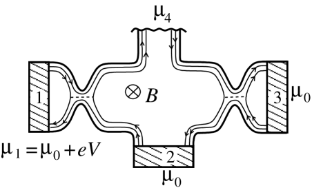
Figure 2.  : A voltage probe at the upper edge generates inelastic scattering or dephasing depending on whether the total instantaneous current or additionally the current at every energy is set to zero. After Texier and Büttiker [24].

4 Cross correlation in the presence of quasi-elastic scattering

Incoherence can be introduced into the coherent scattering approach to electrical conduction with the help of fictitious voltage probes. (see Fig. 2). Ideally a voltage probe maintains zero net current at every instant of time. [ A realistic voltmeter will have a finite response time. However since we are concerned with the low-frequency limit this is of no interest here.] A carrier entering a voltage probe will thus be replaced by a carrier entering the conductor from the voltage probe. Outgoing and incoming carriers are unrelated in phase and thus a voltage probe is a source of decoherence. A real voltage probe is dissipative. If we wish to model dephasing which at low temperatures is due to quasi-elastic scattering we have to invent a voltage probe which preserves energy. de Jong and Beenakker [29] proposed that the probe keeps not only the total current zero but that the current in each energy interval is zero at every instant of time. Noise correlations in the presence of a dephasing voltage probe have been investigated by van Langen and the author for multi-terminal chaotic cavities [17].

In the discussion that follows we will assume, as shown in Fig. 1 that the outer edge channel is perfectly transmitted at both quantum point contacts. Only the inner edge channel is as above transmitted with probability $T_{1}$ at the first quantum point contact and with probability $T_{2}$ at the second quantum point contact. Elastic inter-edge channel scattering is very small as demonstrated in experiments by van Wees et al. [46], Komiyama et al. [47], Alphenaar et al. [48] and Mueller et al. [49] and below we will not address its effect on the cross correlation. For a discussion of elastic interedge scattering in this geometry the reader is referred to the work by Texier and Büttiker [24]. We wish to focus on the effects of quasi-elastic scattering and inelastic scattering. The addition of the outer edge channel has no effect on the noise in a purely quantum coherent conductor. Edge channels with perfect transmission are noiseless [6].

To model quasi-elastic scattering along the upper edge of the conductor we now introduce an additional contact (see Fig. 2). To maintain the current at zero for each energy interval we re-write the Langevin equations Eq. (4) for each energy interval $dE$,

$$\Delta I_{\alpha}(E,t)=\frac{e}{h}[(N_{\alpha}-R_{\alpha\alpha}(E))f_{\alpha}(E,t)-\sum_{\beta\neq\alpha}T_{\alpha\beta}(E)f_{\beta}(E,t)]+\delta I_{\alpha}(E,t)\>.$$ (13)

At the voltage probe we have $\Delta I_{4}(E,t)=0$ and thus the distribution function of contact $4$ is given by

$$f_{4}(E,t)=\bar{f}_{4}(E)+\delta f_{4}(E,t)\>,$$ (14)

where the time-independent part of the distribution function is given by

$$\bar{f}_{4}(E)=\frac{1}{N_{\alpha}-R_{\alpha\alpha}}[\sum_{\alpha=1}^{\alpha=3}T_{4\alpha}f_{\alpha}]\>,$$ (15)

and the fluctuating part of the distribution function is

$$\Delta f_{4}(E,t)=\frac{h}{N_{\alpha}-R_{\alpha\alpha}}\delta I_{4}(E,t)\>.$$ (16)

Here we have taken into account that the distribution functions at contact $1$, $2$ and $3$ are time-independent (equilibrium) Fermi functions. Only the distribution at contact $4$ fluctuates. Additionally, its time-averaged part is a non-equilibrium distribution function. For the simple example considered here it is given by

$$\bar{f}_{4}(E)=\frac{1+T_{1}}{2}f_{1}(E)+\frac{R_{1}}{2}f_{2}(E)\>.$$ (17)

It is a two step distribution function [50, 17] as shown in Fig. 3. Since there is now also a fluctuating part of the distribution function the total fluctuating current at contact $\alpha$ contains according to Eq. (13) also a term $-(e/h)T_{\alpha\beta}(E)\Delta f_{4}(E,t)$. We take the transmission probabilities to be energy independent. Integration over energy gives thus for the fluctuating current at contact $\alpha$

$$\Delta I_{\alpha}=\delta I_{\alpha}-\frac{G_{\alpha 4}}{G_{44}}\delta I_{4}\>.$$ (18)

As a consequence the correlation between the currents at contacts $\alpha$ and $\beta$ in the presence of a quasi-elastic voltage probe is $P^{\rm qe}_{\alpha\beta}=\left\langle\Delta I_{\alpha}\Delta I_{\beta}\right\rangle$ with

$$P^{\rm qe}_{\alpha\beta}=P_{\alpha\beta}-\frac{G_{\alpha 4}}{G_{44}}P_{\beta 4}-\frac{G_{\beta 4}}{G_{44}}P_{\alpha 4}+\frac{G_{\alpha 4}G_{\beta 4}}{G_{44}^{2}}P_{44}\>.$$ (19)

Here $P_{\alpha\beta}$ are the auto-correlations and cross-correlations of the fluctuating currents in the energy resolved Langevin equation Eq. (13). The spectra are evaluated with the help of Eqs. (5) that apply for a completely coherent conductor except that we use the distribution functions $f_{1},f_{2},f_{3}$ and $\bar{f}_{4}(E)$. In this procedure we neglect thus the fluctuations of the distribution function in the evaluation of the intrinsic noise powers $P_{\alpha\beta}$. [This is appropriate for the second order correlations of interest here, but not for the higher order cumulants [51, 52]].

In contrast to Eq. (9) the current-current correlation Eq. (19) is not necessarily negative. Taking into account that the off-diagonal conductances are negative and that the intrinsic spectra $P_{\alpha\beta}$ and $P_{4\beta}$ are negative for cross-correlations, it is clear that the first three terms in Eq. (19) are negative. The forth term, due to the fluctuating distribution in the dephasing contact, is positive. For all examples known to us, it turns out that for a dephasing voltage probe, the first three terms win and the resulting correlation is negative [17]. For the inelastic (physical) voltage probe this is not the case as we demonstrate below.

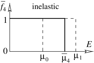
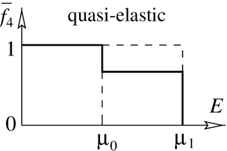
Figure 3.  : Distribution functions in the voltage probe reservoir. For inelastic scattering this an equilibrium distribution function with a potential $\mu_{4}$ determined such that the average current vanishes. For a dephasing voltage probe this is a two step function determined such that the current at the probe vanishes at every energy.

We will not discuss the most general result of Ref. [24] here but instead focus on the fact that such a dephasing probe can generate shot noise even in the case where the quantum coherent sample is noiseless.

5 Quasi-elastic partition noise

Consider the conductor for which the quantum point contacts are both closed for the inner edge channel $T_{1}=0$ and $T_{3}=0$. In this case, at zero temperature, the quantum coherent sample is noiseless. Transmission along each edge state is either one or zero. Now consider the conductor with the dephasing probe. Under the biasing condition considered here, the distribution function $\bar{f}_{4}(E)$ is still a non-equilibrium distribution function and given by $\bar{f}_{4}(E)=\frac{1}{2}f_{1}(E)+\frac{1}{2}f_{2}(E)$. The distribution function at the dephasing contact is similar to a distribution at an elevated temperature with $kT=eV/4$ with $eV$ the voltage applied between contact $1$ and contacts $2$ and $3$. We have $\int dE\bar{f}_{4}(E)(1-\bar{f}_{4}(E))=e|V|/4$. As a consequence the bare spectra $P_{\alpha\beta}$ and $P_{\beta 4}$ are now non-vanishing. Evaluation of the correlation function Eq. (19) gives [24],

$$P^{\rm qe}_{23}=-\frac{e^{2}}{h}|eV|\frac{1}{4}\>.$$ (20)

The electron current incident into the voltage probe from contact $1$ is noise-less. Similarly, the hole current that is in the same energy range incident from contact $2$ is noiseless. However, the voltage probe has two available out-going channels. The noise generated by the voltage probe is thus a consequence of the partitioning of incoming electrons and holes into the two out-going channels. In contrast, at zero-temperature, the partition noise in a coherent conductor is a purely quantum mechanical effect. Here the partioning invokes no quantum coherence and is a classical effect.

We emphasize that a dephasing voltage probe generates zero-temperature, incoherent partition noise whenever it is connected to channels which in a certain energy range are not completely filled. In our example the nonequilibrium filling of the channels incident on the voltage probe arises since the incident channels are occupied by reservoirs at different potentials. For instance a dephasing voltage probe connected to a ballistic wire (with adiabatic contacts) will generate incoherent partition noise if the probabilities for both left and right movers to enter the voltage probe are non-vanishing. If we demand that a dephasing voltage probe sees only left movers [53, 54] (we might add a dephasing voltage probe which sees only right movers) we have a dephasing probe that not only conserves energy but also generates only forward scattering. As long as all incident channels are equally filled such a forward scattering dephasing probe will not generate partition noise.

6 Voltage probe with inelastic scattering

We next compare the results of the energy conserving voltage probe with that of a real (physical) voltage probe. At such a probe only the total current vanishes. The Langevin equations are

$$I_{\alpha}(t)=\sum_{\beta}G_{\alpha\beta}V_{\beta}(t)+\delta I_{\alpha}(t)\>.$$ (21)

where $G_{\alpha\beta}$ are the elements of the conductance matrix and $V_{\beta}(t)$ is the voltage at contact ${\beta}$. The voltages at contacts $1,2$ and $3$ are constant in time $eV_{1}=\mu_{1}$ and $eV_{2}=eV_{3}=\mu_{0}$. But the voltage at contact $4$ is determined by $I_{4}(t)=0$ and is given by

$$V_{4}(t)=\bar{V}_{4}+\delta V_{4}(t)\>.$$ (22)

The time-independent voltage is

$$\bar{V}_{4}=-G_{44}^{-1}\sum_{\beta\neq 4}G_{4\beta}V_{\beta}\>,$$ (23)

and the fluctuating voltage is

$$V_{4}(t)=-G_{44}^{-1}\delta I_{4}(t)\>.$$ (24)

The distribution function in contact $4$ consists of a time-independent part and a fluctuating part. The time-independent distribution is an equilibrium Fermi distribution at the potential $e\bar{V}_{4}=\bar{\mu}_{4}$. For our example we have

$$\bar{V}_{4}=\mu_{0}+\frac{1}{2}(1+T_{1})e|V|\>.$$ (25)

We remark that that this potential is independent of the transmission of quantum point contact 3. The fluctuating currents at the contacts of the sample are

$$\Delta I_{\alpha}(t)=\delta I_{\alpha}(t)-\frac{G_{\alpha 4}}{G_{44}}\delta I_{4}\>.$$ (26)

As a consequence the correlations of the currents are given by an equation which is similar to Eq. (19)

$$P^{\rm in}_{\alpha\beta}=P_{\alpha\beta}-\frac{G_{\alpha 4}}{G_{44}}P_{\beta 4}-\frac{G_{\beta 4}}{G_{44}}P_{\alpha 4}+\frac{G_{\alpha 4}G_{\beta 4}}{G_{44}^{2}}P_{44},\>$$ (27)

but with the important difference that the bare noise spectra are evaluated with the equilibrium Fermi functions $f_{\alpha}$ with $\alpha=1,2,3,4$.

As in the quasi-elastic case, the first three terms are negative and the forth term is positive due to the auto-correlations of the fluctuating voltage in this contact. In the inelastic case we can not consider the case where both $T_{1}$ and $T_{3}$ are zero since this implies that $\mu_{4}=\mu_{1}$. Thus $T_{1}$ must be non-vanishing. On the other hand we are stil free to choose $T_{3}$ to simplify the problem. It is now interesting to consider the case $T_{3}=0$. In this case shot noise is generated at QPC $1$ and the voltage probe generates fluctuating populations in the the two out-going edge channels. The outer edge state leads carriers to contact $3$ and the inner edge state leads carriers to contact $2$. Interestingly, with this choice the first three terms in $P^{\rm in}_{23}$ vanish and the only non-zero term is the forth term arising from the auto-correlations of the voltage fluctuations in contact four. The correlation $P^{\rm in}_{23}$ is thus positive!

In the presence of the voltage probe and for $T_{3}=0$, the correlation at contacts $2$ and $3$ is [24]

$$P^{\rm in}_{23}=+\frac{e^{2}}{h}|eV|\frac{1}{2}T_{1}R_{1}\>.$$ (28)

The autocorrelations are $P^{\rm in}_{22}=P^{\rm in}_{33}=P^{\rm in}_{23}$. Current conservation is obeyed since $P^{\rm in}_{12}=P^{\rm in}_{13}=-2P^{\rm in}_{23}$ and $P^{\rm in}_{11}=4P^{\rm in}_{23}$. Thus the normalized correlation function is $p^{in}_{23}\equiv P^{\rm in}_{23}/(P^{\rm in}_{22}P^{\rm in}_{33})^{1/2}=+1$. Clearly, as a consequence of the fluctuating voltage electrons are injected into the two edge channels in a correlated way.

In the introduction we have remarked that thermal fluctuations are always anti-correlated. Therefore, as we increase the temperature in this conductor but keep the voltage fixed thermal fluctuations should eventually overpower the correlations due to the fluctating potential of the voltage probe. As a consequence, with increasing temperature, the correlation function should change sign. Indeed, a calculation gives [24]

$$P^{\rm in}_{23}=\frac{e^{2}}{h}\bigg{[}-k_{B}T\left(2+{R_{1}}+{R_{1}T_{1}}\right)+\frac{R_{1}T_{1}}{2}{eV}\coth\frac{eV}{2k_{B}T}\bigg{]}\>.$$ (29)

If $k_{B}T=0$ we recover the positive result $P^{\rm in}_{23}=(e^{2}/h)|eV|R_{1}T_{1}/2$ for the shot noise, and if $V=0$ we find $P^{\rm in}_{23}=-(2e^{2}/h)k_{B}T(1+R_{1}/2)$, which is the result of the fluctuation-dissipation theorem: $P^{\rm in}_{23}=2k_{B}T(G^{\rm in}_{23}+G^{\rm in}_{32})$ where [54] $G^{\rm in}_{\alpha\beta}=G_{\alpha\beta}-(G_{\alpha 4}G_{4\beta}/G_{44})$ is the conductance of the three-terminal conductor in the presence of incoherent scattering.

We define $T_{c}$, the critical temperature above which the correlations $P^{\rm in}_{23}$ are negative. For small transmission $T_{1}\ll 1$ we find: $k_{B}T_{c}\simeq|eV|T_{1}/6$, and for large transmission $R_{1}\ll 1$: $k_{B}T_{c}\simeq|eV|R_{1}/4$. The transmission that maximizes the critical temperature is [24] $T_{1}=3-\sqrt{6}\simeq 0.55$. In this case we have: $k_{B}T_{c}^{\rm max}\simeq|eV|(5\sqrt{6}-12)/(2(6\sqrt{6}-12))\simeq|eV|/21.8$. Clearly, it would be intersting to see an experiment which investigates the reverasl of the sign of such a correlation function as a function of temperature. Another possibility is to perform the experiment at a fixed temperature but to make transmission into the voltage probe variable (for instance with the help of a gate). At temperatures so low that intrinsic inelastic scattering can be neglected the theory predicts a negative correlation if the connection is closed. As the contact to the voltage is opend there must exist a critical transmission probability at which the correlation vanishes. Finally for sufficiently large transmission the correlation is positive.

Figure 4.  : Ballistic one-channel wire coupled to reservoirs and capacitively coupled to a gate. After Blanter, Hekking and Büttiker, [55].

7 Dynamic Reversal of the sign of a Current-Current Correlation

The proof that current-current correlations in normal conductors are negative applies only to the white-noise (low-frequency) limit. At finite frequencies it is possible to have positive current-current correlations even at equilibrium. To illustrate this we consider a one-channel ballistic conductor connected adiabatically to two electron reservoirs and capacitively coupled to a gate with capacitance $c$ per unit length. The gate is connected to ground without additional impedance. The conductance matrix of this wire was calculated by Blanter, Hekking and Büttiker [55] combining scattering theory with dynamic screening to determine the electrostatic potential self-consistently in random phase approximation. The conductance matrix determined in this way agrees with a theory based on a Tomonaga-Luttinger Hamiltonian and bosonization [56]. The wire has a length $L$ and a density of states (per unit length) of $\nu_{F}=2/hv_{F}$ where $v_{F}$ is the Fermi velocity. The interaction is described by the parameter

$$g^{2}=\frac{1}{1+e^{2}\nu_{F}/c}\>$$ (30)

which is $1$ in the limit of a very large capacitance $c$ (non-interacting limit) and tends to zero as the capacitance $c$ becomes very small. The parameter $g$ and the density of states determine the static, electro-chemical capacitance [57] of the wire vis-a-vis the gate, $c_{\mu}=g^{2}e^{2}\nu_{F}$. The dynamic conductance matrix is defined as $G_{\alpha\beta}(\omega)=\delta I_{\alpha}(\omega)/\delta V_{\beta}(\omega)$ where $\delta I_{\alpha}(\omega)$ and $\delta V_{\beta}(\omega)$ are the Fourier coefficients of the current at contact $\alpha$ and the voltage at contact $\beta$. Here $\alpha$ and $\beta$ label the contacts, the reservoirs $1$ and $2$ and the gate $3$. At equilibrium the dynamic conductance matrix is related to the current-current fluctuations via the Fluctuation-Dissipation theorem,

$$P_{\alpha\beta}(\omega)={\hbar\omega}\,\,coth{\frac{\hbar\omega}{2kT}}G^{\prime}_{\alpha\beta}(\omega)\>$$ (31)

where $G^{\prime}_{\alpha\beta}(\omega)=(1/2)(G_{\alpha\beta}(\omega)+G^{\star}_{\beta\alpha}(\omega))$ is the real part of the element $G_{\alpha\beta}(\omega)$ of the conductance matrix. Consider now the current-current correlation $P_{12}(\omega)$. In terms of the effective wave-vector $q\equiv\omega g/v_{F}$ Ref. [55] finds

$$G^{\prime}_{12}(\omega)=-\frac{e^{2}}{h}\frac{16g^{2}cos(qL)}{16g^{2}cos^{2}(qL)+4(1+g^{2})^{2}sin^{2}(qL)}\>.$$ (32)

In the zero-frequency limit we have $G^{\prime}_{12}(\omega)=-\frac{e^{2}}{h}$ which is negative as it must be for a conductance determined by a transmission probability. At a critical frequency

$$\omega_{c}=v_{F}\pi/Lg\>.$$ (33)

determined by $qL=\pi$, the real part of this conductance element becomes positive. Hence for $\omega>\omega_{c}$ there exist frequency windows for which the equilibrium currents are positively correlated. We note that in the non-interacting limit $g=1$ this frequency is determined by the time an electron takes to traverse half of the length of the wire, $\tau=L/2v_{F}$. At this frequency the wire is charged by carriers coming in simultaneously from both reservoirs. Increasing the interaction suppresses charging and thus increases this frequency. On the other hand the frequency is inversely proportional to the length of the wire and the frequency tends to zero as the wire length tends to infinity.

Since much of the discussion based on Luttinger theory and bosonization does not take into account the finite size of the sample, we can expect that such theories would in fact predict positive correlations! Indeed if we consider for a moment a Luttinger liquid coupled at a point $x=0$ to a tunneling contact an electron inserted into the wire gives with probability $1/2$ rise to a left (right) going plasma excitation with charge e(1-g)/2 and a right (left) going excitation with charge eg/2. This charges lead to positively correlated currents [58] at $x=\pm L/2$ with a noise spectrum proportional to $(1/4)g(1-g)$. Since the transition from a Luttinger liquid to a normal region leads to reflection of plasma excitations [56] we can expect that a proper treatment of the contacts would restore the expected negative correlations.

The positive dynamic correlations discussed here are only accessible at high frequencies. Is it possible to observe positively correlated currents at low frequencies? The answer is yes and we will now discuss two geometries.

8 Positive Correlations of Dynamic Screening Currents

Consider the classical electrical circuit shown in Fig. 5 in which a node with potential $U$ is at one branch connected via a resistor with resistance $R$ to terminal $1$ and at the other branches via capacitances $C_{1}$ and $C_{2}$ to terminals $2$ and $3$. We are interested in the low-frequency behavior and expand the classical ac-conductance matrix ${\bf G}$ in powers of the frequency

$${\bf G}(\omega)=-i\omega{\bf C}+\omega^{2}{\bf K}+...\>.$$ (34)

The first term is purely capacitive with a capacitance matrix ${\bf C}$. The second term, which is of interest here, is the lowest order in frequency term which is dissipative. For the classical circuit of Fig. 5 it is given by

$${\bf K}=R\left(\begin{array}[]{ccc}C_{\Sigma}^{2}&-C_{1}C_{\Sigma}&-C_{2}C_{\Sigma}\\ -C_{1}C_{\Sigma}&C_{1}^{2}&C_{1}C_{2}\\ -C_{2}C_{\Sigma}&C_{1}C_{2}&C_{2}^{2}\end{array}\right)\;\;.$$ (35)

Here $C_{\Sigma}=C_{1}+C_{2}$. The key point is of course that the off-diagonal elements $K_{23}=K_{32}$ are positive. In view of the fluctuation-dissipation theorem this implies that the correlation of currents at the two capacitive terminals are positively correlated, $P_{23}=2kT\omega^{2}K_{23}=2kT\omega^{2}C_{1}C_{2}R$. A current fluctation leads to charging of the capacitors $C_{1}$ and $C_{2}$ which in turn generates simultaneously current flowing through the two terminals $2$ and $3$ to compensate this charge.

Figure 5.  : Left: A classical three-terminal circuit: One branch is coupled via a resistor $R$ and two branches are coupled with capacitances $C_{1}$ and $C_{2}$ to the node. Right: A cavity coupled via a narrow lead to a reservoir at voltage $V_{0}$ and coupled capacitively to two gates with geometric capacitances $C_{1}$ and $C_{2}$. $U$ is the voltage at node (left) and inside the cavity (right).

The classical circuit can, for example, be viewed as a simple model for the ac currents of a mesoscopic (chaotic) cavity coupled capacitively to two gates with geometrical capacitances $C_{1}$ and $C_{2}$ and connected via a quantum point contact to a particle reservoir. There are mesoscopic corrections to the geometrical capacitances and they are replaced by electrochemical capacitances $C_{\mu,1}$ and $C_{\mu,2}$. Similarly, the classical two terminal resistance $R$ is replaced by a charge relaxation resistance [59]. In a theory that determines the internal potential $U$ of the cavity in random phase approximation both the electrochemical capacitances and the charge relaxation resistances can be expressed in terms of elements of the Wigner-Smith, Jauch-Marchand, time delay matrix [60, 61, 62],

$$N_{\beta\gamma}=\frac{1}{2\pi i}\sum_{\alpha}s_{\beta\alpha}^{\dagger}\frac{ds_{\gamma\alpha}}{dE}.$$ (36)

that characterizes fully the low-frequency charge fluctuations on the cavity [63]. For the mesoscopic cavity the four dynamical transport coefficients of interest are,

$$\begin{array}[]{cc}D=e^{2}\mbox{Tr}N,&C_{\mu,1}=\frac{C_{1}D}{C_{\Sigma}+D},\\ \\ C_{\mu,2}=\frac{C_{2}D}{C_{\Sigma}+D},&R_{q}=\frac{h}{2e^{2}}\frac{\left(\mbox{Tr}N^{2}\right)}{\left(\mbox{Tr}N\right)^{2}}.\\ \end{array}$$ (37)

Replacing $C_{1},C_{2}$ and $R$ in Eqs. (34) and (35) with $C_{\mu,1},C_{\mu,2}$ and $R_{q}$ gives the low frequency response of the mesoscopic cavity. Thus the equilibrium current correlations $P_{12}=P_{21}$ of the mesoscopic cavity are also positively correlated.

Figure 6.  : Quantum point contact in the quantum Hall regime: a single edge is partially transmitted and reflected. Charging of the edge state is probed capacitively with a capacitor at $A$ and second capacitor $B$ which can be in positions I-IV. After Martin and Büttiker [64].

Thus far we have considered frequency dependent equilibrium fluctuations. Martin and Büttiker [64] have investigated the correlation of dynamic screening currents in open conductors. The example considered is shown in Fig. 6. A Hall bar in a high magnetic field is connected to two reservoirs $1$ and $2$. The magnetic field corresponds to a filling factor $\nu=1$ such that the wire is in the integer quantum Hall regime. Backscattering is generated by a quantum point contact. The lines along the edges of the conductor indicate the edge states. Their chirality is indicated by arrows. Two gates $A$ and $B$ are used to probe charge fluctuations capacitively. Four positions $I,II,III,IV$ are considered for gate $B$ whereas gate $A$ is always held at the same position. Charge fluctuations on an edge state will induce capacitive currents on the gates $A$ and $B$.

To keep the discussion simple it is assumed that charge pile up occurs only in the proximity of the gates $A$ and $B$ and that the remaining part of the conductor is charge neutral. The regions where charge pile up can occur are indicated by the volumes $\Omega_{A}$ for gate $A$ and $\Omega_{B}$ for gate $B$. The geometrical capacitance of the gates to the edge states are denoted by $C_{A}$ and $C_{B}$. Again it is possible to express the charge fluctuations with the help of a generalized Wigner-Smith matrix. Whereas in the example of the cavity discussed above, the charge in the entire cavity was of interest, here we are interested only in the charge pile up in the regions $\Omega_{A}$ and $\Omega_{B}$. We are thus interested in local charge fluctuations. As a consequence we now have to consider functional derivatives of the scattering matrix with regard to the local potential [65],

$${\cal N}^{(\eta)}_{\delta\gamma}=\frac{-1}{2\pi}\sum_{\nu}\int_{\Omega_{\eta}}d^{3}{\bf r}\left[s^{\star}_{\nu\delta}(E,U({\bf r}))\frac{\delta s_{\nu\gamma}(E,U({\bf r}))}{e\delta U({\bf r})}\right]$$ (38)

where $\eta=A$ or $\eta=B$ and ${\bf r}$ is in the volume $\Omega_{\eta}$ and $U({\bf r})$ is the electrostatic potential at position ${\bf r}$. For example ${\cal N}^{(A)}_{12}({\bf r})$ is the electron density, at position $\bf{r}$ in volume $\Omega_{A}$, associated with two electron current amplitudes incident from contacts $1$ and $2$. The explicit relation of the charge operator to local wave functions is given in [65] and a detailed derivation is found in Ref. [66].

The density of states of the edge state in region $A$ and $B$ and the electrochemical capacitances are

$$N_{\eta}=\sum_{\gamma}\,\,{\cal N}^{\eta}_{\gamma\gamma}({\bf r}),$$ (39)

$$C_{\mu_{\eta}}=\frac{e^{2}N_{\eta}C_{\eta}}{C_{\eta}+e^{2}N_{\eta}}.$$ (40)

The current correlation at equilibrium at a temperature $kT$ can be brought into the form

$$S_{I_{\alpha}I_{\beta}}=2\omega^{2}C_{\mu_{\alpha}}C_{\mu_{\beta}}R_{q}^{\alpha\beta}kT\>,$$ (41)

where

$$R_{q}^{\alpha\beta}=\frac{h}{2e^{2}}\frac{\sum_{\gamma\delta}{\rm Tr}\left[{\cal N}_{\delta\gamma}^{(\alpha)}({\cal N}_{\delta\gamma}^{(\beta)})^{\dagger}\right]}{{\rm Tr}\left[\sum_{\gamma}{\cal N}_{\gamma\gamma}^{(\alpha)}\right]{\rm Tr}\left[\sum_{\gamma}{\cal N}_{\gamma\gamma}^{(\beta)}\right]}.$$ (42)

For $\alpha=\beta=A$ these equations determine the auto-correlation and for $\alpha=A$ and $\beta=B$ the cross-correlation. In the zero temperature limit in the presence of an applied voltage $|eV|$ between contact $1$ and $2$ we can bring the current-current correlation into the form

$$S_{I_{\alpha}I_{\beta}}(\omega)=2\omega^{2}C_{\mu_{\alpha}}C_{\mu_{\beta}}R_{V}^{\alpha\beta}|eV|\>,$$ (43)

where

$$R_{V}^{\alpha\beta}=\frac{h}{2e^{2}}\frac{{\rm Tr}\left[{\cal N}_{12}^{(\alpha)}({\cal N}_{12}^{(\beta)})^{\dagger}\right]+{\rm Tr}\left[{\cal N}_{21}^{(\alpha)}({\cal N}_{21}^{(\beta)})^{\dagger}\right]}{{\rm Tr}\left[\sum_{\gamma}{\cal N}_{\gamma\gamma}^{(\alpha)}\right]{\rm Tr}\left[\sum_{\gamma}{\cal N}_{\gamma\gamma}^{(\beta)}\right]}.$$ (44)

The electrochemical capacitances are positive and the sign of the current-correlations at the two gates is thus determined by $R_{q}^{\alpha\beta}$ at equilibrium and by $R_{V}^{\alpha\beta}$ in the zero temperature limit in the presence of transport.

  ($i$) ($ii$) ($iii$) ($iv$)   $S^{q}_{I_{A}I_{B}}(\omega)$ $>0$ $=0$ $\geq 0$ $\geq 0$   $S^{V}_{I_{A}I_{B}}(\omega)$ $\geq 0$ $\leq 0$ $=0$ $=0$  

TABLE 1.  : Sign of equilibrium ($S^{q}_{I_{A}I_{B}}(\omega)$) and non- equilibrium ($S^{V}_{I_{A}I_{B}}(\omega)$) current correlations between gates $A$ and $B$ for the four positions of gate $B$ relative to gate $A$.

For the geometry $I$ Ref. [64] finds,

$$R_{q}^{\alpha\beta}=(h/2e^{2})\,\,\,\,\,{\rm and}\,\,\,\,\,R_{V}^{\alpha\beta}=(h/e^{2})TR,$$ (45)

independent of the choice of $\alpha$ and $\beta$. Here $T$ is the transmission probability through the quantum point contact and $R$ is the reflection probability. Thus at equilibrium the charge relaxation resistance is universal and given by $h/2e^{2}$. This results from the fact that a charge accumulated on the edge state near gate $A$ and $B$ can leave the sample only through contact $2$ where we have an interface resistance $h/2e^{2}$ . In the presence of transport, in the zero temperature limit considered here, the charge fluctuations reflect the shot noise and are proportional to $T(1-T)$. In geometry $I$ we find thus both at equilibrium and in the presence of shot noise a positive correlation.

Consider next geometry $II$. Here gate $A$ and $B$ tests charge accumulation due to transmitted and reflected particles. These are mutually exclusive events and Ref. [64] finds,

$$R_{q}^{AA} = R_{q}^{BB}=(h/2e^{2}),$$ (46)

$$R_{q}^{AB} = R_{q}^{BA}=0,$$ (47)

$$R_{V}^{AA} = R_{V}^{BB}=-R_{V}^{AB}=-R_{V}^{BA}=(h/e^{2})TR.$$ (48)

The equilibrium correlations proportional to $R_{q}^{AB}$ are zero, whereas the non-equilibrium correlations given by Eq. (48) are negative. The results for the different geometries are summarized in Table $I$.

The direct relation between charge fluctuations and the resistances $R_{q}$ and $R_{v}$ (see Eqs. (37) and Eqs. (42,44)) makes these quantities useful for many problems. Ref. [66, 67, 68] link these quantities to dephasing times in Coulomb coupled open conductors and Ref.[69] demonstrates, that the dephasing time and relaxation time of a closed double quantum dot capacitively coupled to a mesoscopic conductor is governed by these resistances.

9 Cooper pair partition versus pair breaking noise

Hybrid-structures [30, 31, 32, 33, 34] consisting of a normal conductor and superconductor provide another system in which interactions play an important role in current-current correlations. At a normal-superconducting interface an electron (hole) is reflected as a hole (electron) if it is incident with an energy below the gap of the superconductor. This process, known as Andreev reflection, correlates excitations with different charge. Currents at the normal contacts of such a structure can be written as a sum an electron current $(e)$ and hole current $(h)$. Thus the correlation function $P_{\alpha\beta}$ can be similarly decomposed into four terms,

$$P_{\alpha\beta}=P^{ee}_{\alpha\beta}+P^{hh}_{\alpha\beta}+P^{eh}_{\alpha\beta}+P^{he}_{\alpha\beta}$$ (49)

corresponding to correlations of currents of the same type of quasi-particles and correlations between electron and hole currents. It can be shown that $P^{ee}$ and $P_{hh}$ are negative and $P^{eh}$ and $P^{he}$ are positive. The sign of the correlation depends on the strength of the different contributions. Indeed Anantram and Datta [35] showed that for a simple one-channel normal structure in which the normal part and the superconducting part form a loop penetrated by a flux $\Phi$, that the correlation measured at two normal contacts changes sign as a function of flux. Subsequent investigations based on a single channel Y-structure with a wave splitter which depends on a coupling parameter [70] found that the correlation changes sign and becomes positive as the coupling to the superconductor is decreased [37, 71]. Investigation of a highly asymmetric geometry of an NS-structure in which one of the normal contacts is a tunneling tip found similarly restrictive conditions for positive correlations and moreover indicated that with increasing channel number of the normal conductor it is less and less likely to observe positive correlations [38].

Figure 7.  : A chaotic cavity is connected to two normal ($N_{1}$ and $N_{2}$) reservoirs and and to a superconductor $S$ via quantum point contacts. After Samuelsson and Büttiker [41].

These results pose the question of whether positive correlations are indeed a feature of few channel ballistic systems only and could in fact not be seen in multi-channel systems which are typically also channel mixing. Indeed Nagaev and the author [72] investigating diffusive normal structures, perfectly coupled to the superconductor, and neglecting the proximity effect, found that correlations are manifestly negative, as in purely normal structures. In view of the current interest in sources of entangled massive particles and the detection of entanglement, understanding the correlations generated in hybrid structures is of particular interest [73, 74, 75].

To investigate the sign of current correlations in channel mixing hybrid structures for a wider range of conditions Samuelsson and the author [41] analyzed current correlations in a chaotic cavity using random matrix theory. The system is shown in Fig. 7. A chaotic cavity is coupled via quantum point contacts with $N_{1}=N$ and $N_{2}=N$ open channels at the normal contacts and with $M$ channels to the superconducting contact.

The result of the random matrix calculation is depicted in Fig. 8. In the absence of the proximity effect (broken line in Fig. 8) the ensemble averaged cross-correlation is negative over the entire range of the ratio $2N/M$. This situation is the analog for the chaotic cavity of the negative correlations found in diffusive conductors by Nagaev and the author [72]. The result is dramatically different if the proximity effect plays a role (solid curve of Fig. (8). Now, at least in the limit where the cavity is much better coupled to the superconductor than to the normal reservoirs, the correlations are positive. Due to the multitude of processes contributing to these results a detailed microscopic explanation is difficult. In Ref. [41] Samuelsson and the author present explanations for the limiting behavior ($N\ll M$ and $M\gg N$).

A simple picture emerges if a barrier of strength $\Gamma_{s}$ is inserted into the contact between the cavity and a superconductor (see Fig. 7). The case where there are tunnel barriers in all contacts has been investigated by Boerlin et al. [40]. Here we focus our attention to the case where the contacts to the normal reservoirs are perfect quantum point contacts and only the contact to the superconductor contains a barrier (as shown in the inset of Fig. 9). A simple result is obtained in the limit $2N/M\gg 1$. In this case injected quasi-particles scatter at most once from the superconductor-dot contact and the resulting scattering matrix simplifies considerably. The resulting correlation function is

$$\frac{\langle P_{12}\rangle}{P_{0}}=\frac{M}{2N}R_{eh}(1-2R_{eh})$$ (50)

where $R_{eh}=\Gamma_{S}^{2}/(2-\Gamma_{S})^{2}$ is the Andreev reflection probability of quasiparticles incident in the dot-superconductor contact. There is a crossover from negative to positive correlations that takes place already for $R_{eh}=1/2$, i.e $\Gamma_{S}=2(\sqrt{2}-1)\approx 0.83$, in agreement with the full numerics in Fig. 9. The fact that a ”bad” contact reducing the Andreev reflection is favorable in generating positive correlations seems at first counter intuitive. Below we give a simple discussion to explain this result.

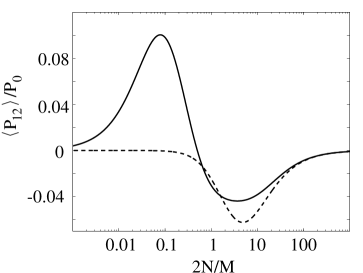
Figure 8.  : Current-current correlation of the chaotic dot junction coupled to the superconductor with $M$ open channels and with normal contacts of $N$ open channels as a function of $2N/M$. In the presence of the proximity effect (solid line) the correlation is positive for $2N<M$. Application of a magnetic flux of the order of a flux quantum suppresses the proximity effect and leads to negative correlations (broken line) independent of the ratio of $N$ and $M$. After P. Samuelsson and M. Büttiker [41].

Eq.(50) is the cross-correlation averaged over an ensemble of cavities. Since the proximity effect plays no role, it must be possible, to derive this result from a purely semiclassical discussion. This statement holds of course not only for the particular geometry of interest here but of all the results obtained in the absence of the proximity effect. A semiclassical theory for chaotic-dot superconductor systems is presented in Ref. [76] not only for the current-current correlations but also for the higher cumulants. Below we focus on the simple result described by Eq. (50).

In the presence of the tunnel barrier at the superconductor-dot contact we can view the superconductor as an injector of Cooper pairs [39]. This picture differs from the Andreev-Bogoliubov-de Gennes picture of correlated electron-hole processes. The (mathematical) transformation between these two pictures is of interest and will be discussed elsewhere. The argument presented below expands a suggestion by Schomerus [77]. We divide time into intervals such that the n-th time slot might contain a Cooper pair $\sigma_{n}=1$ which has successfully penetrated through the barrier and entered the cavity or the n-th time slot is empty, $\sigma_{n}=0$, if the Cooper pair has been reflected. Clearly, we have

$$<\sigma_{n}>\,=<\sigma^{2}_{n}>\,=R_{eh}$$ (51)

where $R_{eh}$ is the Andreev reflection probability. Once the Cooper pair has entered the cavity two processes are possible: either the entire Cooper pair is transmitted into one of the normal contacts giving raise to Cooper pair partition noise or the Cooper pair is split up and one electron leaves through contact $1$ and the other electron leaves through contact $2$. We refer to the contribution to the correlation function by this second process as pair breaking noise. To proceed we assume that each electron has a probability $T_{1}$ to enter contact $1$ and probability $T_{2}=1-T_{1}$ to enter contact $2$. Thus for a symmetric junction $T_{1}=T_{2}=1/2$ an incident Cooper pair contributes with probability $1/2$ to the partition noise and with probability $1/2$ to the pair breaking noise.

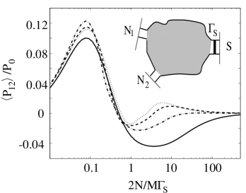
Figure 9.  : Current-current correlation of a chaotic cavity connected to the superconductor via a contact with conductance proportional to $\Gamma_{s}M$ and to two normal reservoirs with $N$ open channels as a function of $2N/M\Gamma_{s}$. The contact transparencies are $\Gamma_{s}=1$ (solid line) $0.8$ (dashed dotted) $0.6$ (dashed line). For large $2N/M\Gamma_{s}$ the correlation crosses over from negative to positive as the transparency $\Gamma_{s}$ is reduced. After P. Samuelsson and M. Büttiker [41].

We now want to write the correlation function in a way that permits us to separate these processes. The charge $Q_{1}$ transferred into contact $1$ over large number of time slots is

$$Q_{1}=\sum_{n}\sigma_{n}(p_{n}+q_{n})$$ (52)

and the charge $Q_{2}$ transferred into contact $2$ is

$$Q_{2}=\sum_{n}\sigma_{n}(1-p_{n}+1-q_{n}).$$ (53)

Here $q_{n}$ and $p_{n}$ denote the two particles comprising the cooper pair. For pair partition we have $p_{n}=q_{n}=1$ or $p_{n}=q_{n}=0$ and for pair breaking we have $p_{n}=1,q_{n}=0$ or $p_{n}=0,q_{n}=1$.

Next we consider the fluctuations of the transferred charge $\Delta Q_{i}=Q_{i}-<Q_{i}>$. The average transmitted charge is $<Q_{i}>=R_{eh}$. For the correlation we find,

$$<\Delta Q_{1}\Delta Q_{2}>\,=\,<\Delta Q_{1}\Delta Q_{2}>_{p}+<\Delta Q_{1}\Delta Q_{2}>_{e}$$ (54)

where the index $p$ denotes the contribution of the pairs which are transmitted in their entierty into lead $1$ or $2$ and $e$ is the average only over the pairs which are broken up and an electron is emitted into each contact. For pair transmission we can distinguish events which emit a pair through the upper lead 1. In this case $\Delta Q_{1}=2\sum_{n}\sigma_{n}-R_{eh}$ and $\Delta Q_{2}=-R_{eh}$ One quarter of all events are of this type. Similarly we can treat the case of pairs emitted through lead 2. Taking into account that $<\sum_{n}\sigma_{n}>=R_{eh}$ we find a pair partition noise

$$<\Delta Q_{1}\Delta Q_{2}>_{p}\,=\,-(1/2)R^{2}_{eh}$$ (55)

Like the partition noise of single electrons in a normal conductor it is negative.

Consider next the pair breaking events. For these events $\Delta Q_{1}=\sum_{n}\sigma_{n}-R_{eh}$ and $\Delta Q_{2}=\sum_{m}\sigma_{m}-R_{eh}$. Onehalf of the time-slots with a Cooper pair are of this type. The correlation contains four terms, $<\sum_{n}\sum_{m}\sigma_{n}\sigma_{m}>=R_{eh}$, $-R_{eh}<\sum_{n}\sigma_{n}>=-R_{eh}R_{eh}$, $-R_{eh}<\sum_{n}\sigma_{n}>=-R_{eh}R_{eh}$, and a term $+R_{eh}R_{eh}$. Thus simultaneous emission of electrons gives rise to a noise

$$<\Delta Q_{1}\Delta Q_{2}>_{e}\,=\,(1/2)R_{eh}(1-R_{eh}).$$ (56)

This contribution to the cross-correlation is positive.

Notice that the pair partition noise is negative and quadratic in $R_{eh}$. The pair breaking process gives a contribution which is linear in $R_{eh}$ for small $R_{eh}$ and thus wins in this limit. To achieve positive correlations it is thus favorably to have a small Andreev reflection probability. Only in this limit can the pair breaking processes overcome the negative partition noise of Cooper pairs and give rise to positive correlations. The full counting statistics is discussed in Ref. [76].

In hybrid superconducting normal structures there are thus several possibilities for a sign reversal of current-current fluctuations. For a cavity that is well coupled to a superconductor (see Fig. (8) application of a magnetic flux reverses the sign from positive to negative. As a function of temperature or applied voltage we can have a sign reversal both for the cavity that is well coupled to the superconductor (see Fig. 8) as well as for the cavity that connects to the superconductor via a tunnel contact (see Fig. (9). For temperatures and voltages large compared to the superconducting gap the structure considered here behaves like a normal structure and exhibits negative correlations.

10 Summary

For non-interacting particles injected from thermal sources there is a simple connection between the sign of correlations and statistics. In contrast to photons, electrons are interacting entities, and we can expect the simple connection between statistics and the sign of current-current correlations to be broken, if interactions play a crucial role.

The standard situation consists of a normal conductor embedded in a zero-frequency external impedance circuit such that the voltages at the contacts can be considered to be constant in time. Under this condition the low frequency current-current cross-correlations measured at reservoirs are negative independent of the geometry, number of contacts and the bias applied to the conductor (as long as we do not depart to far from equilibrium). The negative correlations are a consequence of Fermi-statistics and the unitarity of the scattering matrix. Under these conditions the fluctuations in the potential play no role. We have shown that already the voltage fluctuations at a real voltage contact are sufficient to change the sign of correlations in certain special situations. Carriers injected by the voltage probe are correlated by the fluctuations of the potential of the voltage probe and can in the situation considered overcome the anti-bunching generated by Fermi statistics. We have also pointed out that displacement currents (screening currents) are positively correlated even at small frequencies. The electron-hole correlations generated in a normal conductor by a superconductor can similarly generate positive correlations in situations in which the pair partition noise is overcome by the pair breaking noise.

The fact that interactions can have a dramatic effect on current-current correlations (change even their sign) clearly makes them a promising subject of further theoretical and experimental investigations.

Acknowlegements

The work presented here is to a large extent based on collaborations with Christophe Texier, Andrew Martin and Peter Samuelsson. I thank S. Pilgram, K. E. Nagaev and E. V. Sukhorukov for valuable comments on the manuscript. The work is supported by the Swiss National Science Foundation, the Swiss program for Materials with Novel Properties and the European Network of Phase Coherent Dynamics of Hybrid Nanostructures.

References

- [1] Ya. M. Blanter and M. Büttiker, Physics Reports, 336, 1-166 (2000).
- [2] R. Hanbury Brown and R.Q. Twiss, Nature 177, 27 (1956);
- [3] R. Hanbury Brown and R. Q. Twiss, Nature 178, 1447 (1956).
- [4] A. M. Steinberg, P. G. Kwiat, and R. Y. Chiao, Phys. Rev. Lett. 71, 708 (1993).
- [5] E. M. Prucell, Nature 178, 1449 (1956).
- [6] M. Büttiker, Phys. Rev. Lett. 65, 2901 (1990).
- [7] M. Büttiker, Physica B175, 199 (1991).
- [8] M. Büttiker, Phys. Rev. Lett. 57, 1761 (1986).
- [9] M. Büttiker, IBM J. Res. Developm. 32, 317 (1988).
- [10] V. A. Khlus, Zh. Éksp. Teor. Fiz. 93 (1987) 2179 [Sov. Phys. JETP 66 (1987) 1243].
- [11] G. B. Lesovik, Pis’ma Zh. Éksp. Teor. Fiz. 49 (1989) 513 [JETP Lett. 49 (1989) 592].
- [12] M. Büttiker, Phys. Rev. B46, 12485 (1992).
- [13] R. Landauer and Th. Martin, Physica B 175 (1991) 167; T. Martin and R. Landauer, Phys. Rev. B 45(4), 1742 (1992).
- [14] M. Büttiker, Phys. Rev. Lett. 68, 843, (1992).
- [15] T. Gramespacher and M. Büttiker, Phys. Rev. Lett. 81, 2763 (1998).
- [16] Ya. M. Blanter and M. Büttiker, Phys. Rev. B55, 2127 (1997).
- [17] S. A. van Langen and M. Büttiker, Phys. Rev. B 56, 1680 (1997).
- [18] E. V. Sukhorukov and D. Loss, Phys. Rev. B59, 13054 (1999).
- [19] W. D. Oliver, J. Kim, R. C. Liu, and Y. Yamamoto, Science 284, 299 (1999).
- [20] M. Henny, S. Oberholzer, C. Strunk, T. Heinzel, K. Ensslin, M. Holland, and C. Schönenberger, Science 284, 296 (1999).
- [21] S. Oberholzer, M. Henny, C. Strunk, C. Schönenberger, T. Heinzel, K. Ensslin, and M. Holland, Physica E 6, 314 (2000).
- [22] T. Kodama, N. Osakabe, J. Endo, and A. Tonomura, K. Ohbayashi, T. Urakami, S. Ohsuka, H. Tsuchiya, Y. Tsuchiya and Y. Uchikawa Phys. Rev. A 57, 2781 (1998).
- [23] H. Kiesel, A. Renz and F. Hasselbach, Nature 418, 392 (2002).
- [24] C. Texier and M. Büttiker, Phys. Rev. B 62, 7454 (2000).
- [25] M. Büttiker, Phys. Rev. B 32, 1846 (1985).
- [26] M. Büttiker, Phys. Rev. B 33, 3020 (1986).
- [27] C. W. J. Beenakker and M. Büttiker, Phys. Rev. B46, 1889 (1992).
- [28] R. C. Liu and Y. Yamamoto, Phys. Rev. B50, 17411 (1994).
- [29] M. J. M. de Jong and C. W. J. Beenakker, Physica A 230, 219 (1996).
- [30] X. Jehl, M. Sanquer, R. Calemczuk and D. Mailly, Nature (London) 405 50 (2000).
- [31] A.A. Kozhevnikov, R.J. Shoelkopf, and D.E. Prober, Phys. Rev. Lett. 84 3398 (2000).
- [32] X. Jehl and M. Sanquer, Phys. Rev. B 63, 052511 (2001).
- [33] B. Reulet, A. A. Kozhevnikov, D. E. Prober, W. Belzig, Yu. V. Nazarov, ”Phase Sensitive Shot Noise in an Andreev Interferometer”, cond-mat/0208089
- [34] F. Lefloch, C. Hoffmann, M. Sanquer and D. Quirion, ”Doubled Full Shot Noise in Quantum Coherent Superconductor - Semiconductor Junctions”, cond-mat/0208126
- [35] M. P. Anantram and S. Datta, Phys. Rev. B 53, 16390 (1996).
- [36] Th. Martin, Phys. Lett. A220, 137 (1966).
- [37] J. Torr s and Th. Martin, Eur. Phys. J. B 12, 319 (1999).
- [38] T. Gramespacher and M. Büttiker, Phys. Rev. B 61, 8125 (2000).
- [39] P. Recher, E. V. Sukhorukov, and D. Loss, Phys. Rev. B 63, 165314 (2001).
- [40] J. Börlin , W. Belzig, and C. Bruder , Phys. Rev. Lett. 88, 197001 (2002).
- [41] P. Samuelsson and M. Büttiker, Phys. Rev. Lett. 89, 046601 (2002).
- [42] B. I. Halperin, Phys. Rev. B 25, 2185 (1982).
- [43] M. Büttiker, Phys. Rev. B 38, 9375 (1988).
- [44] M. I. Reznikov, M. Heiblum, H. Shtrikman, and D. Mahalu, Phys. Rev. Lett. 75 3340 (1995).
- [45] A. Kumar, L. Saminadayar, D. C. Glattli, Y. Jin, and B. Etienne, Phys. Rev. Lett. 76, 2778 (1996).
- [46] B. J. van Wees, E. M. M. Willems, L. P. Kouwenhoven, C. J. P. M. Harmans, J. G. Williamson, C. T. Foxon, and J. Harris, Phys. Rev. B 39, 8066 (1989).
- [47] S. Komiyama, H. Hirai, S. Sasa, and T. Fujii, Solid State Commun. 73, 91 (1990).
- [48] B. W. Alphenaar, P. L. McEuen, R. G. Wheeler, and R. N. Sacks, Phys. Rev. Lett. 64, 677 (1990).
- [49] G. Müller, D. Weiss, A. V. Khaetskii, K. von Klitzing, S. Koch, H. Nickel, W. Schlapp, and R. Lösch, Phys. Rev. B 45, 3932 (1992).
- [50] K. E. Nagaev, Phys. Lett. A 169, 103 (1992).
- [51] K. E. Nagaev, ”Boltzmann - Langevin approach to higher-order current correlations in diffusive metal contacts”, cond-mat/0203503
- [52] K. E. Nagaev, P. Samuelsson and S. Pilgram, ”Cascade approach to current fluctuations in a chaotic cavity”, (unpublished). cond-mat/0208147
- [53] M. Büttiker, ”Noise in Mesoscopic Conductors and Capacitors”, Proceedings of the 13th International Conference on Noise in Physical Systems and 1/f-Fluctuations, eds. V. Bareikis and R. Katilius, (Word Scientific, Singapore, 1995). p. 35 - 40.
- [54] M. Büttiker, in ”Resonant Tunneling in Semiconductors: Physics and Applications”, edited by L. L. Chang, E. E. Mendez, and C. Tejedor, (Plenum Press, New York, 1991). p. 213-227.
- [55] Ya. M. Blanter, F.W.J. Hekking, and M. Büttiker, Phys. Rev. Lett. 81, 1925 (1998).
- [56] I. Safi, Ann. Phys. (Paris) 22, 463 (1997).
- [57] M. Büttiker, J. Phys. Condensed Matter 5, 9361 (1993).
- [58] M. Büttiker (unpublished); A. Crepieux and Th. Martin, (unpublished).
- [59] M. Büttiker, H. Thomas, and A. Prêtre, Phys. Lett. A180, 364 (1993).
- [60] E. P. Wigner, Phys. Rev. 98, 145 (1955); F. Smith, Phys. Rev. 118, 349 (1960).
- [61] J. M. Jauch and J. P. Marchand, Helv. Physica Acta 40, 217 (1967).
- [62] Since we are interested in the charge density within a specific region the derivative should be taken with respect to the local (electrostatic) potential, (see Eq. (38)) and not energy. The difference is important in situations where a WKB-approximation does not apply. See also M. Büttiker, Phys. Rev. B27, 6178 (1983).
- [63] M. H. Pedersen, S. A. van Langen, M. Büttiker, Phys. Rev. B 57, 1838 (1998).
- [64] A. M. Martin and M. Büttiker, Phys. Rev. Lett. 84, 3386 (2000).
- [65] M. Büttiker, J. Math. Phys. 37, 4793 (1996).
- [66] M. Büttiker, in ”Quantum Mesoscopic Phenomena and Mesoscopic Devices”, edited by I. O. Kulik and R. Ellialtioglu, (Kluwer, Academic Publishers, Dordrecht, 2000). Vol. 559, p. 211. cond-mat/9911188
- [67] M. Büttiker and A. M. Martin, Phys. Rev. B61, 2737 (2000).
- [68] G. Seelig and M. Büttiker, Phys. Rev. B 64, 245313 (2001).
- [69] S. Pilgram and M. Büttiker, (unpublished). cond-mat/0203340,
- [70] M. Büttiker, Y. Imry and M. Ya. Azbel, Phys. Rev. A 30, 1982 (1984).
- [71] G. B. Lesovik , T. Martin, and G. Blatter , Eur. Phys. J. B 24, 287 (2001).
- [72] K. Nagaev and M. Büttiker, Phys. Rev. B 63 081301, (2001).
- [73] G. Burkard, D. Loss, and E. V. Sukhorukov, Phys. Rev. B 61, 16303 (2000).
- [74] F. Taddei, and R. Fazio, Phys. Rev. B 65, 134522 (2002).
- [75] P. Recher and D. Loss, ”Superconductor coupled to two Luttinger liquids as an entangler for electron spins”, cond-mat/0204501
- [76] P. Samuelsson and M. Büttiker, ”Semiclassical theory of current correlations in chaotic dot-superconductor systems”, (unpublished). cond-mat/0207585
- [77] Private communication by H. Schomerus