Berry phase in Magnetic Superconductors

Abstract

In magnetic systems, electronic bands often acquire nontrivial topological structure characterized by gauge flux distribution in momentum($\mathbf{k}$)-space. It sometimes follows that the phase of the wavefunctions cannot be defined uniquely over the whole Brillouin zone. In this Letter we develop a theory of superconductivity in the presence of this gauge flux both in two- and three-dimensional systems. It is found that the superconducting gap has “nodes” as a function of $\mathbf{k}$ where the Fermi surface is penetrated by a gauge string.

Geometric phases and topology of wavefunctions have been the subject of intensive studies berry ; review . The quantized Hall effect (QHE) in a 2D electron system under a strong magnetic field can be also interpreted in terms of the topological integer called Chern number tknn . If the system has a gap, the Hall conductivity is proportional to the Chern number and is quantized. This nontrivial topology of Bloch waves is not specific to the QHE, but is common and universal in systems with broken time-reversal symmetry. Namely, in magnetic materials with the spin-orbit interaction and/or tilting of spin configuration, there occur many band-crossing points which are locally described as Weyl fermions and act as (anti)monopoles in the momentum-space ohgushi ; onoda ; shindou ; taguchi . The existence of (anti)monopoles means that the Bloch wavefunction cannot be defined in a single gauge choice sakurai . The anomalous Hall effect in ferromagnets represents this topological property of the Bloch wavefunctions ohgushi ; taguchi .

On the other hand, coexistence of magnetic ordering and superconductivity (SC) is found in many materials and is a recent significant issue super . Although detailed analysis of each material is still missing in most of the cases, it is highly desirable to establish the general feature of the SC in systems with broken time-reversal symmetry.

In the present Letter we shall study the SC made out of the Bloch states with nontrivial topology. The quantity of central importance is the gauge flux defined in the momentum space, which is generated by the vector potential $\mathbf{A}_{(n)}(\mathbf{k})=-i\langle\mathbf{k}n|\nabla_{\mathbf{k}}|\mathbf{k}n\rangle$, where $|\mathbf{k}n\rangle$ is the Bloch wavefunction of the $n$-th band. Band indices are represented by subcripts with parenthesis. This $\mathbf{A}_{(n)}(\mathbf{k})$ represents an overlap of the two wavefunctions separated infinitestimally in the $\mathbf{k}$-space, i.e. the Berry phase connection. The gauge flux is defined as $\mathbf{B}_{(n)}(\mathbf{k})=\nabla_{\mathbf{k}}\times\mathbf{A}_{(n)}(\mathbf{k})$. It is worth noting that the monopole density $\rho_{(n)}(\mathbf{k})=\frac{1}{2\pi}\nabla_{\mathbf{k}}\cdot\mathbf{B}_{(n)}(\mathbf{k})$ is nonzero, and is given by $\rho_{(n)}(\mathbf{k})=\sum_{l}q_{ln}\delta(\mathbf{k}-\mathbf{k}_{ln})$, where $q_{ln}$ is an integer called the strength of the monopole berry . The monopoles are located at “diabolical points” berry ; volovik , where bands touch each other. The monopole and antimonopole act as the source and the sink of the gauge flux $\mathbf{B}(\mathbf{k})$, respectively, as in Fig. 1(a). In general, the up- and down-spins have different band structures; therefore, $\mathbf{A}$, $\mathbf{B}$, and $\rho$ are spin-dependent, and we shall write as $\mathbf{A}_{\alpha}$, $\mathbf{B}_{\alpha}$ and $\rho_{\alpha}$, where $\alpha$ is a spin index.

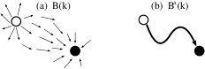
Figure 1: Distribution of (a) $\mathbf{B}(\mathbf{k})$ and (b) $\mathbf{B}^{\Delta}(\mathbf{k})$. The open and the solid circles represent the monopoles and the antimonopoles, respectively.

The question we address below is an effect of this gauge flux $\mathbf{B}(\mathbf{k})$ on the SC properties. In order to characterize topological properties of the gap function $\Delta(\mathbf{k})$, we define a vector potential $\mathbf{A}^{\Delta}(\mathbf{k})=-\nabla_{\mathbf{k}}\text{Im}\ln\Delta(\mathbf{k})=-\nabla_{\mathbf{k}}\text{arg}\Delta(\mathbf{k})$, a flux density $\mathbf{B}^{\Delta}=\nabla_{\mathbf{k}}\times\mathbf{A}^{\Delta}(\mathbf{k})$, and a monopole density $\rho^{\Delta}(\mathbf{k})=\frac{1}{2\pi}\nabla_{\mathbf{k}}\cdot\mathbf{B}^{\Delta}(\mathbf{k})$. For the moment, we assume that $\Delta(\mathbf{k})$ is nonvanishing in almost all over the BZ noteDelta ; we shall discuss later what happens without this assumption. As explained later, distribution of $\mathbf{B}^{\Delta}(\mathbf{k})$ is confined into strings as in Fig. 1(b), due to bosonic nature of $\Delta(\mathbf{k})$. The main result of the present Letter is that in 3D topological structures of the gap function $\Delta(\mathbf{k})$ is solely determined from that of the wavefunction: $\rho^{\Delta}_{\alpha\beta}(\mathbf{k})=\rho_{\alpha}(\mathbf{k})-\rho_{\beta}(-\mathbf{k})$. It reflects the fact that $\Delta_{\alpha\beta}(\mathbf{k})$ represents a pairing between $(\mathbf{k},\alpha)$ and $(-\mathbf{k},\beta)$ electrons. Thus if the band structure in the normal state is known, we can immediately calculate the monopole density $\rho^{\Delta}_{\alpha\beta}(\mathbf{k})$, irrespective of details of the attractive potential. The monopole density $\rho^{\Delta}_{\alpha\beta}(\mathbf{k})$ tells us about zeros and phases of the gap function.

Henceforth we focus on the SC where only one component of the gap function is nonzero: (i) singlet SC, (ii) triplet SC with $\Delta_{\uparrow\downarrow}\neq 0$, $\Delta_{\uparrow\uparrow}=\Delta_{\downarrow\downarrow}=0$, and (iii) triplet SC with $\Delta_{\uparrow\uparrow}\neq 0$, $\Delta_{\uparrow\downarrow}=\Delta_{\downarrow\downarrow}=0$ note-triplet . The case (iii) is appropriate for half-metallic magnetic SC. In the singlet (triplet) SC, we have $\Delta(\mathbf{k})=\Delta(-\mathbf{k})$ ($\Delta(\mathbf{k})=-\Delta(-\mathbf{k})$), implying $\mathbf{B}^{\Delta}(\mathbf{k})=\mathbf{B}^{\Delta}(-\mathbf{k})$, and $\rho^{\Delta}(\mathbf{k})=-\rho^{\Delta}(-\mathbf{k})$ note-delta . We note that the time-reversal symmetry breaking is a necessary condition for nontrivial topology of the gap function. In (iii), broken time-reversal symmetry is assumed from the outset. We have $\rho_{\uparrow\uparrow}^{\Delta}(\mathbf{k})=\rho_{\uparrow}(\mathbf{k})-\rho_{\uparrow}(-\mathbf{k})$. Thus, inversion symmetry must be broken to have nonzero $\rho^{\Delta}_{\uparrow\uparrow}$. In (i) and in (ii) we have $\rho^{\Delta}_{\uparrow\downarrow}(\mathbf{k})=\rho_{\uparrow}(\mathbf{k})-\rho_{\downarrow}(-\mathbf{k})$. Hence in nonmagnetic SC, $\rho^{\Delta}_{\uparrow\downarrow}(\mathbf{k})$ vanishes. In magnetic SC, including both ferromagnets and antiferromagnets, $\rho_{\uparrow\downarrow}^{\Delta}(\mathbf{k})$ is nonzero.

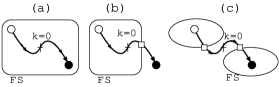
Figure 2: Monopoles (open circles), antimonopoles (solid circles) for $\Delta(\mathbf{k})$, and the Fermi surface. The open squares represent point nodes on the Fermi surface.

Let us consider the distribution of $\mathbf{B}^{\Delta}(\mathbf{k})$. $\mathbf{B}^{\Delta}(\mathbf{k})=-\nabla_{\mathbf{k}}\times\nabla_{\mathbf{k}}\text{arg}\Delta(\mathbf{k})$ is nonzero only when $\Delta=0$, i.e. $\text{Re}\Delta=\text{Im}\Delta=0$, which determines a curve in the 3D BZ in general (Fig. 1 (b)). Distribution of $\mathbf{B}^{\Delta}(\mathbf{k})$ is like a Dirac string, starting from a monopole and terminating at an antimonopole. In contrast, $\mathbf{B}(\mathbf{k})$ does not share this feature; distribution of $\mathbf{B}(\mathbf{k})$ spreads over the BZ (Fig. 1 (a)). Now we discuss the relation among the Fermi surface (FS), the (anti)monopoles and the Dirac string. For any closed surface $S$ in the BZ, the total flux penetrating it is quantized. We take the FS as $S$ for gapless systems. When the total flux penetrating one of the FS’s is nonzero, the gap function cannot be expressed as continuous. It is quite contrary to our conventional view note-2 . Because $\rho^{\Delta}(\mathbf{k})=-\rho^{\Delta}(-\mathbf{k})$, a FS symmetric with respect to $\mathbf{k}=0$ encloses zero monopoles in total, and $\Delta(\mathbf{k})$ can be continuous on this FS (Fig. 2(a)). There are, however, two cases where the Dirac strings penetrate the FS’s. One is the case with broken inversion as well as time-reversal symmetry. Then, the FS is not symmetric with respect to $\mathbf{k}=0$, and can enclose monopoles with nonvanishing strength (Fig. 2 (b)). The other is a pair of FS’s symmetric with respect to $\mathbf{k}=0$. It is possible that one FS encompasses a monopole and the other encompasses an antimonopole (Fig. 2(c)). For example, if one of the FS encloses a monopole of unit strength, a Dirac string starting from this monopole necessarily penetrates the FS. An intersection of this curve with the FS is nothing but a point node. This string can intersect the FS more than once, and the number of point nodes on this FS should be odd. The nonvanishing total flux implies that $\Delta(\mathbf{k})$ cannot be a single continuous function on each FS. The FS should be divided into regions, in each of which $\Delta$ is continuous.

Here we remark on “conventional” nodes in anisotropic SC. Line nodes appear when $\text{Re}\Delta$ and $\text{Im}\Delta$ have a common real factor $f(\mathbf{k})$ as $\Delta(\mathbf{k})=f(\mathbf{k})[\text{Re}g(\mathbf{k})+i\text{Im}g(\mathbf{k})]$. Zeros of $f(\mathbf{k})$ determine a surface, whose intersection with the FS is a line node. It does not affect $\mathbf{B}^{\Delta}(\mathbf{k})$, because $\nabla\text{Im}\ln\Delta(\mathbf{k})=\nabla\text{Im}\ln g(\mathbf{k})$. Hence, only point nodes are concluded from the gauge flux argument. Difference of nonmagnetic SC from magnetic SC lies only in absence of magnetic monopoles; in nonmagnetic SC, Dirac strings necessarily form loops, which may cross the boundary of the BZ. There are many experimental methods to get information on point nodes. In particular, heat conductivity measurements tell us about the direction of the nodes izawa . When the positions of the nodes are known, care must be taken to assign the phase of $\Delta(\mathbf{k})$ for magnetic SC, because our theory asserts that $\Delta(\mathbf{k})$ need not be continuous on the FS. Group-theoretical classifications of gap functions in su ; vg do not apply to the SC with nontrivial topology, since they assume that gap functions are continuous. It would be interesting to classify all possible multivalued gap functions.

To see why topological structure of the wavefunction is inherited by the gap function, we note the following. If the wavefunction is a continuous function of $\mathbf{k}$, there is no monopole. Thus, if there is a monopole, we should divide a surface surrounding it into regions, in each of which the wavefunction is continuous kohmoto . This resembles Dirac monopoles wy , where the vector potential cannot be a single continuous function in the whole space. This “patch” structure of the wavefunctions remains in the gap function via the BCS term in the Hamiltonian.

To understand this mechanism in detail, we start with a 2D model and generalize it to 3D. Similar topological arguments as we have developed in 3D are also possible in 2D as well. In 2D, we define a Chern number and a total vorticity of $\Delta(\mathbf{k})$ as $\text{Ch}=\frac{1}{2\pi}\int_{\text{BZ}}d^{2}\mathbf{k}B(\mathbf{k})_{z}$ and $\nu=\frac{1}{2\pi}\int_{\text{BZ}}d^{2}\mathbf{k}B^{\Delta}(\mathbf{k})_{z}$, respectively. We can show that the total vorticity $\nu_{\alpha\beta}$ of the gap function $\Delta_{\alpha\beta}$ is the sum of the Chern numbers for spin $\alpha$ and for spin $\beta$: $\nu_{\alpha\beta}=\text{Ch}_{\alpha}+\text{Ch}_{\beta}$ note-2D . We shall explain how this result comes out in the singlet SC on the 2D model proposed by Haldane haldane as an illustrative example. We take this model because it is the minimal model which exhibits nontrivial topological structure of wavefunctions without a uniform magnetic field. It is a tight-binding model on the honeycomb lattice. Because there are two sublattices, the Hamiltonian is written as a $2\times 2$ matrix, which is conveniently expressed with the Pauli matrices $\bm{\sigma}$ as $H(\mathbf{k})=vI+\mathbf{w}\cdot\bm{\sigma}$, where $v=2t_{2}\cos\phi\sum_{j}\cos(\mathbf{k}\cdot\mathbf{b}_{j})$, $w_{1}=t_{1}\sum_{j}\cos(\mathbf{k}\cdot\mathbf{a}_{j})$, $w_{2}=t_{1}\sum_{j}\sin(\mathbf{k}\cdot\mathbf{a}_{j})$, and $w_{3}=M-2t_{2}\sin\phi\sum_{j}\sin(\mathbf{k}\cdot\mathbf{b}_{j})$, where $\mathbf{a}_{1}=a(1,0)$, $\mathbf{a}_{2}=a(-\frac{1}{2},\frac{\sqrt{3}}{2})$, $\mathbf{a}_{3}=-\mathbf{a}_{1}-\mathbf{a}_{2}$, $\mathbf{b}_{1}=\mathbf{a}_{2}-\mathbf{a}_{3}$, $\mathbf{b}_{2}=\mathbf{a}_{3}-\mathbf{a}_{1}$, $\mathbf{b}_{3}=\mathbf{a}_{1}-\mathbf{a}_{2}$. $t_{1}$, $t_{2}$, $M$, $\phi$ are constants. The Pauli matrices are not associated with spins, but with the sublattice structure. We set $M=0$ and $0<\phi<\pi$. Time-reversal symmetry is broken by a staggered flux, while the uniform field is absent. This staggered flux is not necessarily external; staggered flux can be realized by a spontaneous magnetic moment in the material itself, through spin-chirality and/or spin-orbit coupling ohgushi ; taguchi . Let us calculate the Chern number for the lower band. By dividing the BZ into two regions $V_{\pm}$ as in Fig. 3, where $\mathbf{k}_{\pm}^{0}=\pm\frac{2\pi}{a}(\frac{1}{3},\frac{1}{3\sqrt{3}})$ are two inequivalent corners of the BZ, we can write down the eigenvector of the lower band as $\mathbf{v}_{+}=\frac{1}{\sqrt{2|\mathbf{w}|(|\mathbf{w}|-w_{3})}}\left(\begin{array}[]{r}w_{3}-|\mathbf{w}|\\ w_{1}+iw_{2}\end{array}\right)$, for $\mathbf{k}\in V_{+}$, and $\mathbf{v}_{-}=\frac{1}{\sqrt{2|\mathbf{w}|(|\mathbf{w}|+w_{3})}}\left(\begin{array}[]{r}-w_{1}+iw_{2}\\ w_{3}+|\mathbf{w}|\end{array}\right)$, for $\mathbf{k}\in V_{-}$. There remains some freedom in the division of the BZ. Because $\mathbf{v}_{\pm}$ is ill-defined only at $\mathbf{k}_{\mp}^{0}$, respectively, we are free to deform this division as long as $\mathbf{k}^{0}_{\mp}\not\in V_{\pm}$. This corresponds to the gauge degree of freedom. At $\mathbf{k}\in V_{+}\cap V_{-}$, two choices of the wavefunction are different by a phase factor $e^{i\phi(\mathbf{k})}\mathbf{v}_{+}=\mathbf{v}_{-}$, i.e., $\mathbf{A}_{+}-\mathbf{A}_{-}=-\nabla_{\mathbf{k}}\phi(\mathbf{k})$, where $e^{i\phi(\mathbf{k})}=\frac{w_{1}-iw_{2}}{\sqrt{w_{1}^{2}+w_{2}^{2}}}$. Thus, we get $\text{Ch}=\oint_{\partial V_{+}}(\mathbf{A}_{+}-\mathbf{A}_{-})\cdot\frac{\text{d}\mathbf{k}}{2\pi}=-\oint_{\partial V_{+}}\frac{\text{d}\phi(\mathbf{k})}{2\pi}=-1$ haldane . The nonzero Chern number implies that the wavefunction cannot be written as a single function for the entire BZ. This also affects the definition of field operators $a_{(i)\mathbf{k}}$. Second-quantized Hamiltonian is written as ${\cal H}=\sum_{\mathbf{k},i,j}c_{\mathbf{k}j}^{\dagger}H_{ji}(\mathbf{k})c_{\mathbf{k}i}$. Field operators $a_{(i)\mathbf{k}}$ are written as $a_{(i)\mathbf{k}}=\sum_{j}v^{\dagger}_{(i)j}(\mathbf{k})c_{j\mathbf{k}}$. Let $a_{\mathbf{k}\pm}$ denote the annihilation operators for the lower band when $\mathbf{k}\in V_{\pm}$. Then, $e^{i\phi(\mathbf{k})}\mathbf{v}_{+}=\mathbf{v}_{-}$ yields $a_{\mathbf{k}+}=e^{i\phi(\mathbf{k})}a_{\mathbf{k}-}$ at $\mathbf{k}\in V_{+}\cap V_{-}$.

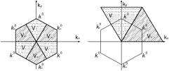
Figure 3: Division of the Brillouin zone of the Haldane model into two regions $V_{+}$ and $V_{-}$.

We now consider the singlet SC on the lower band. In conventional formalism in the BCS theory of SC, it is assumed that the field operators are continuous in the whole BZ; it is no longer true in the present case. We assume that the Fermi energy crosses only the lower band. The BCS pairing term in the Hamiltonian is

$$\sum_{\mathbf{k}\in V_{+}}\Delta(\mathbf{k})_{+}a_{\mathbf{k}+\uparrow}^{\dagger}a_{-\mathbf{k}-\downarrow}^{\dagger}+\sum_{\mathbf{k}\in V_{-}}\Delta(\mathbf{k})_{-}a_{\mathbf{k}-\uparrow}^{\dagger}a_{-\mathbf{k}+\downarrow}^{\dagger}.$$ (1)

Singlet SC implies that $\Delta(\mathbf{k})_{+}=\Delta(-\mathbf{k})_{-}$ for $\mathbf{k}\in V_{+}$, i.e. $\Delta$ is an even function of $\mathbf{k}$. The guiding principle to study topological structure of $\Delta(\mathbf{k})$ is the gauge invariance, corresponding to the freedom in the division of the BZ. It is equivalent to require that the BCS term is continuous at the overlap of two regions; we get $\Delta(\mathbf{k})_{+}=e^{2i\phi(\mathbf{k})}\Delta(\mathbf{k})_{-}$ for $\mathbf{k}\in V_{+}\cap V_{-}$. The total vorticity $\nu$ is

$$\nu=-\sum_{m=\pm}\oint_{\partial V_{m}}\frac{\text{d}\text{arg}\Delta(\mathbf{k})_{m}}{2\pi}=\frac{-1}{2\pi}\oint_{\partial V_{+}}\text{d}\text{arg}\left(\frac{\Delta_{+}}{\Delta_{-}}\right)$$

$$=-2\oint_{\partial V_{+}}\frac{\text{d}\phi(\mathbf{k})}{2\pi}=2\text{Ch}=-2.$$ (2)

Nonzero $\nu$ implies that $\Delta(\mathbf{k})$ can never be expressed as a single continuous function for the entire BZ. To see what the gap function looks like, we take an example of an on-site attraction: ${\cal H}_{U}=-U\sum_{i}n_{i\uparrow}n_{i\downarrow}$. We assume that there are two hole pockets surrounding $\mathbf{k}_{\pm}^{0}$ each. The attractive potential $V(\mathbf{k},\mathbf{k}^{\prime})$ for the lower band is factorized as a product of a function of $\mathbf{k}$ and that of $\mathbf{k}^{\prime}$. We obtain thereby $\Delta(\mathbf{k})_{\pm}=C\frac{w_{1}(\mathbf{k})\mp iw_{2}(\mathbf{k})}{|\mathbf{w}(\mathbf{k})|}\ \ \ (\mathbf{k}\in V_{\pm})$, where $C$ is a complex constant. This has two vortices at $\mathbf{k}=\mathbf{k}_{\pm}^{0}$, with vorticity $-1$ each. The spin Hall conductivity $\sigma_{xy}^{s}$ spinHall can be calculated as $\sigma_{xy}^{s}=0$; it is quantized when $\Delta(\mathbf{k})\neq 0$ on the FS, and $\sigma_{xy}^{s}$ can be nonzero in general.

We can construct simple 3D models starting from the Haldane’s model. For example, we set $w_{1}=t_{1}\sum_{j}\cos(\mathbf{k}\cdot\mathbf{a}_{j})$, $w_{2}=t_{1}\sum_{j}\sin(\mathbf{k}\cdot\mathbf{a}_{j})$, $w_{3}=-2t_{2}\cos(k_{z}c)\sum_{j}\sin(\mathbf{k}\cdot\mathbf{b}_{j})$ in the Hamiltonian $H=\mathbf{w}\cdot\bm{\sigma}$, where $c$ is the lattice constant in the $c$-direction. This is a tight-binding model on a stacked honeycomb lattice with hopping along $\pm\mathbf{a}_{j}$ (nearest-neighbor) and $\pm\mathbf{b}_{j}\pm(0,0,c)$; the latter hopping acquires $\pi/2$ phase if it is clockwise in the hexagonal plaquette. This model has $\rho=\sum_{\alpha,\beta=\pm}\beta\delta(\mathbf{k}-\mathbf{k}_{\alpha}^{0}+\beta\frac{\pi}{2c}\hat{\mathbf{c}})$, leading to $\rho^{\Delta}=2\rho\neq 0$. In some range of parameters, some of the FS’s encircle a monopole or antimonopole, and the total flux is nonzero for them.

So far we have dealt with noninteracting systems. One may wonder if the topological properties of $\Delta(\mathbf{k})$ discussed above are robust against interactions. In general, robustness of physical phenomena originated from topology is guaranteed by an existence of integer topological numbers, which remain unchanged under an adiabatic change of the Hamiltonian. Although this adiabatic principle usually applies to gapful systems, it applies also to Fermi liquid with interactions. In Fermi liquid, bare electrons turn to quasiparticles which are well-defined near the FS. (Even with interactions, the FS is topologically stable in the momentum space. See Fig. 1 in volovik2 .) The BCS theory is founded on this Fermi liquid theory, and the gap function $\Delta(\mathbf{k})$ is defined in terms of these quasiparticles. The total strength of $\Delta(\mathbf{k})$-monopoles inside the FS is a surface integral of a well-defined function $-\frac{1}{2\pi}\nabla_{\mathbf{k}}\times\nabla_{\mathbf{k}}\text{arg}\Delta(\mathbf{k})$ over the FS, and it remains a well-defined integer even when we include interactions and when $\Delta(\mathbf{k})$ vanishes far from the FS. When we start with noninteracting systems, and adiabatically switch on interactions, this integer remain the same for certain range of the strength of the interactions. We note that also the total strength of monopoles for the wavefunction inside the FS remains an integer in the presence of interactions. Its generalized definition in the presence of interactions is $\frac{1}{24\pi^{2}}\epsilon_{\mu\nu\lambda\gamma}\text{Tr}\int_{S}dS^{\lambda}G\partial_{k_{\mu}}G^{-1}G\partial_{k_{\nu}}G^{-1}G\partial_{k_{\lambda}}G^{-1}$ where $G(i\omega,\mathbf{k})$ is the one-particle Matsubara Green’s function, and $S$ is the three-dimensional surface surrounding the FS in the four-dimensional frequency-momentum space $(\omega,\mathbf{k})$ (see Eq. (65) in volovik2 ). It is a well-defined integer, and topologically stable volovik2 . After applying the Stokes’ theorem, the integrand is finite only on the FS, and the integral is equal to the number of monopoles inside the FS. In 3D, Fermi liquid picture is valid even with interactions, and modification of Fermi velocity $v_{F}$ or of quasiparticle residue $Z$ does not change the number of monopoles inside the FS. Thus the total monopole strength remains unchanged. It changes only when the topology of the FS’s changes.

Let us discuss on applicability of our theory to real materials. As mentioned above, we should search through magnetic SC with (a) equal-spin pairing without inversion symmetry or (b) opposite-spin pairing. The case (a) is likely in ferromagnetic SC, while (b) is likely in antiferromagnetic SC. Band structure calculations have been concentrating on energy eigenvalues on high-symmetry directions. Almost no attention has been paid to existence of band-touching points, or to phases of wavefunctions. Thus, we do not have at present sufficient information to see which materials are candidates for our theory. In order to consider how often nontrivial topological structure appears, we should instead resort to simplified models. In onoda , the authors consider a ferromagnetic tight-binding model on the 2D square lattice with $t_{2g}$ orbitals, with physically reasonable values of parameters. The gauge flux $B(\mathbf{k})_{z}$ has sharp peaks, where the bands approach each other in energy. If we go to the 3D by adding an extra dimension along $k_{z}$, the bands will touch each other at some points, because band-touching points (diabolical points) has codimension three volovik ; volovik2 . Actually in shindou , the diabolical points, i.e. the (anti)monopoles, are found in a model for an antiferromagnet. These points are topologically stable. Thus nontrivial topology of the wavefunctions and the gap functions, as discussed in the present Letter, is expected in many materials.

We can argue exciton condensation in the similar way. In 2D, total vorticity of the order parameter is equal to the difference of Chern numbers of the bands involved. In 3D, the monopole density of the order parameter is the difference of those for wavefunctions of the two bands.

In conclusion, we considered the SC in a band with nontrivial topology. It is formulated in terms of a gauge flux distribution in the $\mathbf{k}$-space. Although the gap function $\Delta(\mathbf{k})$ depends on a detail of attractive potential, topological structure of $\Delta(\mathbf{k})$ is determined solely from that of the normal-state wavefunction. The effect of disorder is an interesting issue, and is left for future studies.

- (1) M. V. Berry, Proc. R. Soc. Lond. A 392, 45 (1984).
- (2) A. Shapere and F. Wilczek, Geometric Phases in Physics (World Scientific, Singapore, 1989).
- (3) D. J. Thouless, M. Kohmoto, M. P. Nightingale, and M. den Nijs, Phys. Rev. Lett. 49, 405 (1982).
- (4) K. Ohgushi, S. Murakami and N. Nagaosa, Phys. Rev. B 62, R6065 (2000).
- (5) M. Onoda and N. Nagaosa, J. Phys. Soc. Jpn. 71, 19 (2002).
- (6) R. Shindou and N. Nagaosa, Phys. Rev. Lett. 87, 116801 (2001).
- (7) Y. Taguchi et al., Science 291, 2573 (2001).
- (8) J. J. Sakurai, Modern Quantum Mechanics (Addison-Wesley, 1994) p.140.
- (9) S. S. Saxena et al., Nature (London) 406, 587 (2000); C. Pfleiderer et al., ibid. 412, 58 (2001); A. T. Savici et al., Phys. Rev. B 66, 014524 (2002); Y. Kitaoka et al., J. Phys. Chem. Solids 63, 1141 (2002).
- (10) G. E. Volovik, JETP Lett. 46, 98 (1987).
- (11) In general triplet SC, we consider , which is a product of two gaps. It has a monopole density .
- (12) It means that there is no 3D region with .
- (13) In the pairing with opposite spins , this gives a constraint . Therefore, the pairing with opposite spins is prohibited when the normal-state wavefunction does not satisfy this relation.
- (14) As for the freedom of local gauge transformation , it is natural to choose the gauge so that is continuous, if possible. What we have shown is that in some cases cannot be continuous in any gauge choice.
- (15) K. Izawa et al., Phys. Rev. Lett. 89, 137006 (2002).
- (16) G. E. Volovik and L. P. Gor’kov, Sov. Phys. JETP 61, 843 (1985).
- (17) M. Sigrist and K. Ueda, Rev. Mod. Phys. 63, 239 (1991).
- (18) M. Kohmoto, Ann. Phys. (NY) 160, 343 (1985).
- (19) T. T. Wu and C. N. Yang, Phys. Rev. D12, 3845 (1975).
- (20) In 2D, physical meaning of is the following. A vortex of is defined as a point where and the phase winding of around it is nonzero. We can call this phase winding as a vorticity. The total vorticity is just a summation of vorticity of all the zeros of in the whole BZ. Physically the gap is appreciable only near the FS. Hence, when , it is most probable to have vortices far from the FS to reduce loss of the condensation energy. It is related to the situation when we remove the assumption of nonvanishing in the BZ. The relation no longer holds, because becomes ill-defined. In some sense, vorticies can escape into regions with vanishing , and no effect on physics is left behind. Thus, the total vorticity does not affect low-energy physics of SC in 2D.
- (21) F. D. M. Haldane, Phys. Rev. Lett. 61, 2015 (1988).
- (22) T. Senthil, J. B. Marston, M. P. A. Fisher, Phys. Rev. B 60, 4245 (1999); N. Read and D. Green, ibid. 61, 10267 (2000).
- (23) G. E. Volovik, Phys. Rep. 351, 195 (2001).