Kinetics of the shear banding instability in startup flows

Abstract

Motivated by recent experiments on semi-dilute wormlike micelles, we study the early stages of the shear banding instability using the non-local Johnson-Segalman model with a “two-fluid” coupling to concentration. We perform a linear stability analysis for coupled fluctuations in shear rate $\dot{\gamma}$, micellar strain $\underline{\underline{W}}$ and concentration $\phi$ about an initially homogeneous state. This resembles the Cahn-Hilliard (CH) analysis of fluid-fluid demixing, though we discuss important differences. First assuming the homogeneous state to lie on the intrinsic constitutive curve, we calculate the “spinodal” onset of instability in sweeps along this constitutive curve. We then consider startup “quenches” into the unstable region. Here the instability in general occurs before the intrinsic constitutive curve can be attained so we analyse the fluctuations with respect to the time-dependent homogeneous startup flow, to find the selected length and time scales at which inhomogeneity first emerges. In the uncoupled limit, fluctuations in $\dot{\gamma}$ and $\underline{\underline{W}}$ are independent of those in $\phi$, and are unstable when the intrinsic constitutive curve has negative slope; but no length scale is selected. For the coupled case, this instability is enhanced at short length scales via feedback with $\phi$ and a length scale is selected, consistently with the recent experiments. The unstable region is then broadened by an extent that increases with proximity to an underlying (zero-shear) CH demixing instability. Far from demixing, the broadening is slight and the instability is still dominated by $\delta\dot{\gamma}$ and $\delta\underline{\underline{W}}$ with only small $\delta\phi$. Close to demixing, instability sets in at very low shear rate, where it is demixing triggered by flow.

I Introduction

For many complex fluids, the intrinsic constitutive curve of shear stress $\Sigma$ as a function of shear rate $\dot{\gamma}$ is non-monotonic, admitting multiple values of shear rate at common stress. For example, Cates’ model for semi-dilute wormlike micelles Cates (1990) predicts that the steady shear stress decrease above a critical $\dot{\gamma}=\dot{\gamma}_{\rm c1}$. At very high shear rates, fast relaxation processes must eventually restore an increasing stress Spenley and Cates (1994); Spenley et al. (1993). See curve ACEG of Fig. 1. For the range $\dot{\gamma}_{\rm c1}<\dot{\gamma}<\dot{\gamma}_{\rm c2}$ in which the stress decreases, steady homogeneous flow (Fig. 2a) is unstable Yerushalmi et al. (1970). For an applied shear rate $\bar{\dot{\gamma}}$ in this unstable range, Spenley, Cates and McLeish Spenley et al. (1993) proposed that the system separates into high and low shear rate bands ($\dot{\gamma}_{\rm h}$ and $\dot{\gamma}_{\ell}$) with relative volume fractions satisfying the applied shear rate $\bar{\dot{\gamma}}$. (Fig. 2b.) The steady state flow curve then has the form ABFG. Within the banding regime, BF, a change in the applied shear rate adjusts the relative fraction of the bands, while the stress $\Sigma_{\rm sel}$ (common to both) remains constant. Several constitutive models augmented with interfacial gradient terms have captured this behaviour- Olmsted et al. (2000); Lu et al. (2000); Olmsted and Lu (1997); Olmsted and Goldbart (1992); Pearson (1994); Yuan (1999); Spenley et al. (1996).

Figure 1: Schematic flow curve for wormlike micelles.

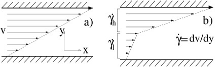
Figure 2: (a) Homogeneous shear rate and (b) banded profiles.

Experimentally, this scenario is well established for shear-thinning wormlike micelles Berret et al. (1994a); Callaghan et al. (1996); Grand et al. (1997). The steady state flow curve has a well defined, reproducible plateau $\Sigma_{\rm sel}$. Coexistence of high and low viscosity bands has been observed by NMR spectroscopy Callaghan et al. (1996); Mair and Callaghan (1996a, b); Britton and Callaghan (1997). Further evidence comes from small angle neutron scattering Berret et al. (1994b); Schmitt et al. (1994); Cappelaere et al. (1997); Berret et al. (1998); Rehage and Hoffmann (1991); Berret et al. (1994a); and from flow birefringence (FB) Decruppe et al. (1995); Makhloufi et al. (1995); Decruppe et al. (1997); Berret et al. (1997), which reveals a (quasi) nematic birefringence band coexisting with an isotropic one. The nematic band of FB has commonly been identified with the low viscosity band of NMR; but see Fischer and Callaghan (2001, 2000).

Here we consider banding formation kinetics. Experimentally Berret et al. (1994a); Berret (1997); Grand et al. (1997); Lerouge et al. (1998); Decruppe et al. (2001); Lerouge et al. (2000); Berret and Porte (1999), in rapid upward stress sweeps the shear rate initially follows the steady state flow curve (AB in Fig. 1) before departing for stresses $\Sigma>\Sigma_{\rm sel}$ along a metastable branch (BC). When this branch starts to level off (hinting of an unstable branch for $\dot{\gamma}\stackrel{{\scriptstyle>}}{{\scriptstyle\sim}}\dot{\gamma}_{\rm c1}$) the shear rate finally “top-jumps”. Under shear startup in the metastable region $\dot{\gamma}_{\ell}<\dot{\gamma}\stackrel{{\scriptstyle<}}{{\scriptstyle\sim}}\dot{\gamma}_{\rm c1}$, the stress first rapidly attains the metastable branch BC (sometimes via oscillations), before slowly decaying onto the steady-state plateau $\Sigma_{\rm sel}$ via a “sigmoidal” envelope $\exp[-(t/\tau_{\rm NG})^{\alpha}]$, with stretching exponent $\alpha$. The time scale $\tau_{\rm NG}$ greatly exceeds the Maxwell time $\tau$ of linear rheology, but is smaller for shear rates $\dot{\gamma}$ closer to $\dot{\gamma}_{\rm c1}$; for most systems the stretching exponent is in the range $1.5\stackrel{{\scriptstyle<}}{{\scriptstyle\sim}}\alpha\stackrel{{\scriptstyle<}}{{\scriptstyle\sim}}3$. In the data of Berret and Porte (1999), for example, $\tau_{\rm NG}\sim(\dot{\gamma}-\dot{\gamma}_{\ell})^{-p}$ and $\alpha\approx 2$ throughout the metastable range, with a crossover to $\alpha\approx 1$ for $\dot{\gamma}\stackrel{{\scriptstyle>}}{{\scriptstyle\sim}}\dot{\gamma}_{\rm c1}$ signifying onset of instability. In more dilute systems Decruppe et al. (2001) the onset of instability can be marked by a huge stress overshoot subsiding rapidly to $\Sigma_{\rm sel}$ via damped oscillations.

In the same experiments Decruppe et al. (2001) the stress overshoot coincided with pronounced concentration fluctuations that first emerged perpendicular to the shear compression axis, at a selected length scale $O(1\mu\rm{m})$. These fluctuations were attributed by the authors of Ref. Decruppe et al. (2001) to the Helfand-Fredrickson Helfand and Fredrickson (1989) coupling of concentration to flow. Although this mechanism has not, to date, been widely employed in the theory of shear banding – an important exception being Schmitt et al. (1995) (discussed below) – it has been recognised elsewhere Brochard and de Gennes (1977); Helfand and Fredrickson (1989); Doi and Onuki (1992); Milner (1993); Wu et al. (1991); Clarke and McLeish (1998); Beris and Mavrantzas (1994); Sun et al. (1997); Tanaka (1996) as an important feature of two components systems with widely separated relaxation times (e.g. polymer and solvent). The slow component (polymer; for our purposes micelles) tends to migrate to regions of high stress; if the plateau modulus increases with polymer concentration ($dG/d\phi>0$), positive feedback enhances concentration fluctuations perpendicular to the shear compression axis (as seen in Ref. Decruppe et al. (2001)) and (sometimes) shifts the spinodal of any nearby Cahn-Hilliard (CH) demixing instabilityClarke and McLeish (1998).

Further evidence for concentration coupling comes from the slight upward slope Berret et al. (1998) in the stress plateau BF of many wormlike micellar systems. This is most readily explained (in planar shear at least) by a concentration difference between the coexisting bands Schmitt et al. (1995); Olmsted and Lu (1997). Any coupling to concentration has important implications for the kinetics of macroscopic band formation, due to the large time scales involved in diffusion.

In this paper we model the initial stages of banding formation in the unstable regime. We use the non-local Johnson-Segalman (d-JS) model Johnson and Segalman (1977); Olmsted et al. (2000) for the dynamics of the micellar stress, since this is the simplest tensorial model that admits a flow curve of negative slope. To incorporate concentration coupling, we use a two-fluid model Brochard and de Gennes (1977); Milner (1991); de Gennes (1976); Brochard (1983) for the relative motion of the micelles and solvent. We perform a linear stability analysis (similar in spirit to the CH calculation for conventional liquid-liquid demixing) for coupled fluctuations in shear rate, micellar stress and concentration about an initially homogeneous shear state. We calculate the “spinodal” boundary of the region in which these fluctuations are unstable. We then consider startup “quenches” into the unstable region, predicting the length and time scales at which inhomogeneity first emerges. We also discuss the physical nature of the growing instability, according to whether its eigenvector is dominated by the flow variables or by concentration.

The two-fluid d-JS model to be studied in this paper was introduced and analysed briefly by us in a previous letter let . In this work we discuss more fully the model’s origin and approximations, and give detailed numerical and analytical arguments supporting the results announced in Ref. let .

For simplicity we consider only fluctuation wavevectors in the velocity gradient direction, $\underline{k}=k\hat{\underline{y}}$, and (separately) the vorticity direction $\underline{k}=k\hat{\underline{z}}$. (The stability of the latter in fact turns out to be unaffected by shear in our model.) Indeed, the spinodal is commonly defined using only these fluctuations for which $\underline{k}.\underline{x}=0$  Onuki (1989)(since any component in the flow gets advected onto the velocity gradient direction), though this restriction is less relevant inside the unstable region where fluctuations can grow on a time scale similar to that of advection.

The paper is structured as follows. In section II we introduce the model and describe its intrinsic constitutive curves. In Sec. IV) we perform a linear stability analysis for slow shear rate sweeps along the intrinsic constitutive curve, to define the spinodal onset of instability. In Sec. V we consider shear startup “quenches” into the unstable region. We conclude in section VI.

II The Model

The existing literature contains several approaches for coupling concentration and flow Brochard and de Gennes (1977); Helfand and Fredrickson (1989); Doi and Onuki (1992); Milner (1993); Wu et al. (1991); Clarke and McLeish (1998); Beris and Mavrantzas (1994). The two-fluid model considered by us follows closely that of Milner Milner (1993), although we extend his work slightly by including a Newtonian contribution to the micellar stress, for reasons discussed in Sec. IV.3.1. (Milner was mainly interested in slow shear phenomena, for which the Newtonian terms are unimportant.)

The basic assumption of the two-fluid model is a separate force balance for the micelles (velocity $\underline{v}_{\,\rm m}$) and the solvent (velocity $\underline{v}_{\,\rm s}$) within any element of solution. These are added to give the force balance for the centre of mass velocity

$$\underline{v}=\phi\underline{v}_{\,\rm m}+(1-\phi)\underline{v}_{\,\rm s},$$ (1)

and subtracted for the relative velocity

$$\underline{v}_{\,\rm rel}=\underline{v}_{\,\rm m}-\underline{v}_{\,\rm s},$$ (2)

which in turn specifies the concentration fluctuations. We give these dynamical equations in Sec. II.2 below. First, we specify the free energy.

II.1 Free energy

In a sheared fluid, one cannot strictly define a free energy because shear drives the system out of equilibrium. Nonetheless, for realistic experimental shear rates many of the internal degrees of freedom of a polymeric solution relax very quickly compared with the rate at which they are perturbed by the externally moving constraints. Assuming that such a separation of time-scales exists, one can effectively treat these fast variables as equilibrated. By integrating over them, one can define a free energy for a given fixed configuration of the slow variables. For our purposes, the relevant slow variables are the fluid momentum $\rho\underline{v}$ and micellar concentration $\phi$ (which are both conserved and therefore truly slow in the hydrodynamic sense), and the micellar strain $\underline{\underline{W}}$ (which is slow for all practical purposes). More precisely $\underline{\underline{W}}$ is the local strain that would have to be reversed in order to relax the micellar stress:

$$\underline{\underline{W}}=\underline{\underline{E}}.\underline{\underline{E}}^{T}-\underline{\underline{\delta}},\;\mbox{ with }\;\delta\underline{r}^{\prime}=\underline{\underline{E}}.\delta\underline{r}$$ (3)

where $\delta\underline{r}^{\prime}$ is the deformed vector corresponding to the undeformed vector $\delta\underline{r}$.

The resulting free energy is assumed to comprise separate kinetic, osmotic and elastic components:

$$F=F^{\rm K}(\underline{v})+F^{\rm o}(\phi)+F^{\rm e}(\underline{\underline{W}}).$$ (4)

The kinetic component is

$$F^{\rm K}(\underline{v})=\tfrac{1}{2}\int d^{3}x\rho\underline{v}^{2}.$$ (5)

The osmotic component is

$$F^{\rm o}(\phi) = \int d^{3}x\left[f(\phi)+\frac{g}{2}(\underline{\nabla}\phi)^{2}\right]$$ (6)

$$\approx \tfrac{1}{2}\int d^{3}q\,(1+\xi^{2}q^{2})f^{\prime\prime}|\phi(q)|^{2},$$

where $f^{\prime\prime}$ is the osmotic susceptibility and $\xi$ is the equilibrium correlation length for concentration fluctuations. The elastic component is

$$F^{\rm e}(\underline{\underline{W}})=\tfrac{1}{2}\int d^{3}xG(\phi){\rm tr}\left[\underline{\underline{W}}-\log(\underline{\underline{\delta}}+\underline{\underline{W}})\right]$$ (7)

in which $G(\phi)$ is the plateau modulus.

II.2 Dynamical equations

We now specify the dynamics. In any fluid element, the forces and stresses on the micelles are as follows:

1. The viscoelastic stress $\underline{\underline{\sigma}}$ of the micellar backbone:

   $$\underline{\underline{\sigma}}=2(\underline{\underline{W}}+\underline{\underline{\delta}}).\frac{\delta F^{\rm e}}{\delta\underline{\underline{W}}}=G(\phi)\underline{\underline{W}}.$$ (8)

2. The osmotic force $\phi\underline{\nabla}[\delta F^{\rm o}/\delta\phi]$ which induces conventional cooperative micellar diffusion and a “non-linear elastic force” $\phi\underline{\nabla}[\delta F^{\rm e}/\delta\phi]$.

3. A Newtonian stress $2\,\phi\,\eta_{\,\rm m}\,\underline{\underline{D}}_{\,\rm m}^{0}$ from fast micellar relaxations such as Rouse modes, where

   $$\underline{\underline{D}}_{\,\rm m}^{0}=\underline{\underline{D}}_{\,\rm m}-\tfrac{1}{3}\underline{\underline{\delta}}\,{\rm Tr}\underline{\underline{D}}_{\,\rm m},$$ (9)

   and

   $$\underline{\underline{D}}_{\,\rm m}=\tfrac{1}{2}\left[\underline{\nabla}\,\underline{v}_{\,\rm m}+(\underline{\nabla}\,\underline{v}_{\,\rm m})^{T}\right].$$ (10)

   We call $\eta_{\,\rm m}$ the “Rouse viscosity” (distinct from the zero shear viscosity of the total micellar stress). $\eta_{\,\rm m}$ is assumed to be independent of $\phi$, but is prefactored by the extensive factor $\phi$.

4. The drag force $\zeta(\phi)\underline{v}_{\,\rm rel}$ impeding the relative motion of micelles and solvent. Scaling theory de Gennes (1975) suggests $\zeta\sim 6\pi\eta\xi^{-2}$ where $\eta$ is the mean viscosity defined in Eqn. 14 below.

5. Stress due to gradients in the hydrostatic pressure $p$.

The overall micellar force balance equation is thus:

$$\rho_{\rm m}\,\phi\,\left(\partial_{t}+\underline{v}_{\,\rm m}.\underline{\nabla}\right)\underline{v}_{\,\rm m}=\underline{\nabla}.G(\phi)\,\underline{\underline{W}}-\phi\,\underline{\nabla}\frac{\delta F(\phi)}{\delta\phi}+2\,\underline{\nabla}.\,\phi\,\eta_{\,\rm m}\,\underline{\underline{D}}_{\,\rm m}^{0}-\zeta(\phi)\,\underline{v}_{\,\rm rel}-\phi\underline{\nabla}p.$$ (11)

Likewise, for the solvent we have the Newtonian viscous stress, the drag force and the hydrostatic pressure:

$$\rho_{\rm s}(1-\phi)\left(\partial_{t}+\underline{v}_{\,\rm s}.\underline{\nabla}\right)\underline{v}_{\,\rm s}=2\underline{\nabla}.\,(1-\phi)\,\eta_{\,\rm s}\,\underline{\underline{D}}_{\,\rm s}^{0}+\zeta(\phi)\underline{v}_{\,\rm rel}-(1-\phi)\underline{\nabla}p.$$ (12)

These equations contain the basic assumption of “dynamical asymmetry”, i.e. that the viscoelastic stress acts only on the micelles and not on the solvent. Adding them, and assuming equal mass densities $\rho_{\rm m}=\rho_{\rm s}=\rho$, we obtain the overall force balance equation for the centre of mass motion

$$\rho\,\left(\partial_{t}+\underline{v}.\underline{\nabla}\right)\underline{v}-\rho\underline{v}_{\,\rm rel}\underline{v}.\underline{\nabla}\phi+\rho\phi(1-\phi)\underline{v}_{\,\rm rel}.\underline{\nabla}\underline{v}_{\,\rm rel}=\underline{\nabla}.G(\phi)\,\underline{\underline{W}}-\phi\,\underline{\nabla}\frac{\delta F(\phi)}{\delta\phi}+2\,\underline{\nabla}.\,\eta\,\underline{\underline{D}}^{0}+2\,\underline{\nabla}.\,\tilde{\eta}\,\underline{\underline{D}}_{\,\rm rel}^{0}-\underline{\nabla}p$$ (13)

in which $\underline{\underline{D}}^{0}$ and $\underline{\underline{D}}_{\,\rm rel}^{0}$, defined analogously to $\underline{\underline{D}}_{\,\rm m}^{0}$ in Eqns. 9 and 10 above, are the traceless symmetrised shear rate tensors for the centre of mass and relative velocity respectively. We have also defined

$$\eta=\phi\eta_{\,\rm m}+(1-\phi)\eta_{\,\rm s}$$ (14)

and

$$\tilde{\eta}=\phi(1-\phi)(\eta_{\,\rm m}-\eta_{\,\rm s}).$$ (15)

The equal and opposite drag forces have cancelled each other in Eqn. 13, which is essentially the Navier-Stokes’ equation generalised to include osmotic stresses. The pressure $p$ is fixed by incompressibility,

$$\underline{\nabla}.\underline{v}=0.$$ (16)

We attach a cautionary note to Eqn. 13. The right hand side (RHS) is the net force acting on the fluid element. The LHS, however, equals the usual convective inertial force plus the two terms in $\underline{v}_{\,\rm rel}$. We consider this to be an unsatisfactory aspect of the two-fluid model that is seldom acknowledged in the literature. One might argue that the separate advected derivatives of Eqns. 11 and 12 should have $\underline{v}.\underline{\nabla}\underline{v}_{\rm i}$ in place of $\underline{v}_{\rm i}.\underline{\nabla}\underline{v}_{\rm i}$ (for ${\rm i}\in{\rm m,s}$). This still leaves the correction $-\underline{v}_{\,\rm rel}\underline{v}.\underline{\nabla}\phi$ on the LHS of Eqn. 13 and does not improve the approximation. In this paper, however, we consider only small fluctuations about a homogeneous shear state (in which $\underline{v}_{\,\rm rel}=0$), and the correction terms are truly negligible.

Subtracting the micellar and solvent Eqns. 11 and 12 (with each predivided by its own volume fraction) gives the relative motion, which in turn specifies the concentration fluctuations:

$$(\partial_{t}+\underline{v}.\underline{\nabla})\phi=-\underline{\nabla}.\phi(1-\phi)\underline{v}_{\,\rm rel}=-\underline{\nabla}.\frac{\phi^{2}(1-\phi)^{2}}{\zeta(\phi)}\left[-\underline{\nabla}\frac{\delta F}{\delta\phi}+\frac{1}{\phi}\underline{\nabla}.G(\phi)\underline{\underline{W}}+2{\mathcal{N}}_{1}(\underline{\underline{D}}^{0})+2{\mathcal{N}}_{2}(\underline{\underline{D}}_{\,\rm rel}^{0})\right].$$ (17)

${\mathcal{N}}_{1}$ and ${\mathcal{N}}_{2}$ are the following Newtonian terms:

$${\mathcal{N}}_{1}(\underline{\underline{D}}^{0})=\frac{\eta_{\,\rm m}}{\phi}\underline{\nabla}.\phi\underline{\underline{D}}^{0}-\frac{\eta_{\,\rm s}}{1-\phi}\underline{\nabla}.(1-\phi)\underline{\underline{D}}^{0}$$ (18)

and

$${\mathcal{N}}_{2}(\underline{\underline{D}}_{\,\rm rel}^{0})=\left(\frac{\eta_{\,\rm m}}{\phi}+\frac{\eta_{\,\rm s}}{1-\phi}\right)\underline{\nabla}.\phi(1-\phi)\underline{\underline{D}}_{\,\rm rel}^{0}.$$ (19)

We have neglected the inertia in $\underline{v}_{\,\rm rel}$ since it is small compared with the drag force $\zeta\underline{v}_{\,\rm rel}$ neg (a). The osmotic contribution to the first term in the square brackets of Eqn. 17 shows that micelles diffuse down to gradients in the chemical potential, as in the usual CH description. The second term states that micelles diffuse in response to gradients in the viscoelastic stress. As described by Helfand and Fredrickon Helfand and Fredrickson (1989), this provides a mechanism whereby micelles can diffuse up their own concentration gradient: the parts of an extended molecule that are in regions of lower viscosity will, during the process of relaxing to equilibrium, move more than those parts mired in a region of higher visosity and concentration. A relaxing molecule therefore on average moves towards the higher concentration region. This provides a mechanism whereby shear can enhance concentration fluctuations, and is the essential physics of the two fluid model.

For the dynamics of the viscoelastic micellar backbone strain we use the phenomenological d-JS model Johnson and Segalman (1977); Olmsted et al. (2000):

$$(\partial_{t}+\underline{v}_{\,\rm m}.\underline{\nabla})\underline{\underline{W}}=a(\underline{\underline{D}}_{\,\rm m}.\underline{\underline{W}}+\underline{\underline{W}}.\underline{\underline{D}}_{\,\rm m})+(\underline{\underline{W}}.\underline{\underline{\Omega}}_{\,\rm m}-\underline{\underline{\Omega}}_{\,\rm m}.\underline{\underline{W}})+2\underline{\underline{D}}_{\,\rm m}-\frac{\underline{\underline{W}}}{\tau(\phi)}+\frac{l^{2}}{\tau(\phi)}\underline{\nabla}^{2}\underline{\underline{W}},$$ (20)

where $2\underline{\underline{\Omega}}_{\,\rm m}=\underline{\nabla}\underline{v}_{\,\rm m}-(\underline{\nabla}\underline{v}_{\,\rm m})^{T}$ with $(\underline{\nabla}\underline{v}_{\,\rm m})_{\alpha\beta}\equiv\partial_{\alpha}(v_{\rm m})_{\beta}$. $\tau(\phi)$ is the Maxwell time. The length $l$ could, for example, be set by the mesh-size or by the equilibrium correlation length for concentration fluctuations. Here we assume the former, since the dynamics of the micellar conformation are more likely to depend on gradients in molecular conformation than in concentration. The equilibrium correlation length $\xi$ of course still enters our analysis, through the concentration free energy of Eqn. 6. Together, $l$ and $\xi$ set the length scale of any interfaces. In the absence of concentration coupling this non-local term involving $l$ is needed to reproduce a steady banded state with a uniquely selected stress Olmsted et al. (2000), although other treatments Yuan (1999); Dhont (1999) have used alternative forms for non-local terms that also give a uniquely selected stress. The slip parameter $a$ measures the non-affinity of the molecular deformation, i.e. the fractional stretch of the polymeric material with respect to that of the flow field. For $|a|<1$ (slip) the intrinsic constitutive curve in planar shear is capable of the non-monotonicity of Fig. 1. We use Eqns. 13, 16, 17 and 20 as our model for the remainder of the paper.

II.3 Flow geometry. Boundary conditions

We consider idealised planar shear bounded by infinite plates at $y=\{0,L\}$ with $(\underline{v},\underline{\nabla}v,\underline{\nabla}\wedge\underline{v})$ in the $(\hat{\underline{x}},\hat{\underline{y}},\hat{\underline{z}})$ directions. The boundary conditions at the plates are as follows. For the velocity we assume there is no slip. For the concentration we assume

$$\partial_{y}\phi=\partial^{3}_{y}\phi=0.$$ (21)

which ensures (in zero shear at least) zero flux of concentration at the boundaries. Following Olmsted et al. (2000), for the micellar strain we assume

$$\partial_{y}W_{\alpha\beta}=0\;\forall\;\alpha,\beta.$$ (22)

Conditions 21 and 22 together ensure zero concentration flux at the boundary even in shear. For controlled shear rate conditions (assumed throughout)

$$\bar{\dot{\gamma}}=\int_{0}^{L}dy\dot{\gamma}(y)={\rm constant.}$$ (23)

II.4 Model parameters

Parameter	Symbol $Q$	Value at $\phi=0.11$	$\frac{d\log Q}{d\log\phi}$
Rheometer gap	$L$	$0.15\mbox{\,mm}$	0
Maxwell time	$\tau$	$0.17\mbox{\,s}$	1.1
Plateau modulus	$G$	$232\mbox{\,Pa}$	2.2
Density	$\rho$	$10^{3}\mbox{\,kg\,m}^{-3}$	0
Solvent viscosity	$\eta_{\,\rm s}$	$10^{-3}\mbox{\,kg\,m}^{-1}\mbox{s}^{-1}$	0
Rouse viscosity	$\eta_{\,\rm m}$	$0.4\mbox{\,kg\,m}^{-1}\mbox{s}^{-1}$	0
Mesh size	$l$	2.6$\times 10^{-8}\mbox{m}$	-0.73
Diffusion coefficient	$D$	$3.5\times 10^{-11}\mbox{m}^{2}\mbox{s}^{-1}$	0.77
Drag coefficient	$\zeta$	$2.4\times 10^{12}\mbox{kg\,m}^{-3}\mbox{\,s}^{-1}$	1.54
Correlation length	$\xi$	$6.0\times 10^{-7}$m	-0.77
Slip parameter	$a$	$0.92$	0

Table 1: Experimental values of the model’s parameters at volume fraction $\phi=0.11$ (column 3). Scaling laws for the dependence of each parameter upon $\phi$ (column 4). In most calculations we use the reference values of column 3 at $\phi=0.11$, then tune $\phi$ using the scaling laws of column 4. Only where stated do we allow the parameters to vary independently.

Values for the model parameters are taken as follows. We assume the solvent viscosity $\eta_{\,\rm s}$ and density $\rho$ to be those of water. We take the plateau modulus $G$ and the Maxwell time $\tau$ from linear rheology ler (a) at $\phi=0.11$ on CTAB(0.3M)/${\rm NaNO}_{3}\rm{(1.79M)}$/H₂O. We estimate the Rouse viscosity $\eta_{\,\rm m}$ from the (limited data on the) high shear branch of the flow curve of a closely related system ler (a). The mesh size is estimated to be $l\approx(k_{B}T/G)^{1/3}$ de Gennes (1975). In fact this form is only truly valid for a good solvent, although in the interests of simplicity we assume it to be good approximation even for systems closer to demixing. We take the diffusion coefficient $D$ and the equilibrium correlation length $\xi$ from dynamic light scattering (DLS) data Candau et al. (1985) on CTAB/KBr/H₂O, at a comparable micellar volume fraction. We calculate the drag coefficient $\zeta=6\pi\eta\xi^{-2}$ de Gennes (1975). We fix the slip parameter $a=0.92$ by comparing our intrinsic constitutive curve in the semi-dilute regime to that of Cates’ model for wormlike micelles Cates (1990). We then have realistic values for all parameters, at $\phi=0.11$ (table 1).

Exploring this large parameter space is a daunting prospect so we shall not, in general, vary the parameters independently. Instead we simply tune the single parameter $\phi$, relying on known semi-dilute scaling laws for the dependence of the other parameters upon $\phi$ (column 4 of table 1). For simplicity we assume that the slip parameter $a$ is independent of $\phi$. We rescale stress, time and length so that $G(\phi=0.11)=1$, $\tau(\phi=0.11)=1$, and $L=1$, where $L$ is the rheometer gap ($0.15{\rm mm}$) used in Ref. ler (a). We also often eliminate $\rho$ in favour of the Reynolds time $\tau_{\rm d}=\rho L^{2}/\eta_{s}$. In total the model has $8$ scaled parameters.

II.5 intrinsic constitutive curves

In planar shear, the stationary homogeneous solutions to Eqns. 13, 16, 17 and 20 for given $\dot{\gamma}$ and $\phi$ are $\underline{v}_{\,\rm rel}=0$ and

$$W_{xy} = \frac{\dot{\gamma}\tau(\phi)}{1+b\dot{\gamma}^{2}\tau^{2}(\phi)},$$

$$W_{yy} = -\frac{1}{(1+a)}\frac{b\dot{\gamma}^{2}}{1+b\dot{\gamma}^{2}}$$

$$W_{xx} = \frac{1+a}{a-1}W_{yy},$$

$$W_{zz} = W_{xz}=W_{yz}=0,$$ (24)

where

$$b=1-a^{2}.$$ (25)

The total shear stress is the sum of the micellar stress and a Newtonian component:

$$\Sigma(\dot{\gamma},\phi)=G(\phi)W_{xy}+{\eta}(\phi)\dot{\gamma}.$$ (26)

This defines a set of intrinsic constitutive curves $\Sigma(\dot{\gamma},\phi)$ (dashed lines in Fig. 3). The criterion for the non-monotonicity of $W_{xy}$ to dominate the Newtonian term ${\eta}(\phi)\dot{\gamma}$ and cause non-monotonicity in the overall stress $\Sigma$ is ${\eta}(\phi)<\tfrac{1}{8}G(\phi)\tau(\phi)$. As $\phi$ is reduced, therefore, the region of negative slope narrows, terminating in a “critical” point at $\phi=\phi_{\rm c}\approx 0.015$. The same qualitative trend has been seen in CPCl/NaSal/brine Berret et al. (1994a).

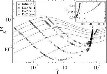
Figure 3: intrinsic constitutive curves for $\phi=0.11$,$0.091,0.072,0.053,0.034,0.015$ (dashed lines, downwards). Spinodals for: the uncoupled limit $\zeta\to\infty$ ($\circ$); coupled model with $D(\phi=0.11)$ taken from the DLS data (table 1) ($\square$); coupled model with $D$ artificially reduced ($\lozenge$,$\vartriangle$). Inset: enlargement at high $\dot{\gamma}$.

III Uncoupled limit; Instabilities; Positive feedback

In the limit of infinite drag, i.e. $\zeta\to\infty$ at fixed $f^{\prime\prime}(\phi)$, the relative motion between micelles and solvent is switched off, disabling concentration fluctuations. In the slightly different limit of $\zeta\to\infty$ at fixed micellar diffusion coefficient

$$D=\frac{\phi^{2}(1-\phi)^{2}f^{\prime\prime}}{\zeta},$$ (27)

the concentration still fluctuates, but independently of the rheological variables. Eqn. 17 then reduces to the CH equation (with a $\phi$-dependent mobility). Independently of $\delta\phi$, the shear rate and micellar stress together obey uniform-$\phi$ d-JS dynamics Radulescu and Olmsted (2000); Olmsted et al. (2000); Radulescu and Olmsted (1999). Accordingly, two separate instabilities are possible:

1. Demixing instability

   For $D<0$, concentration has its own CH demixing instability, governed primarily by the free energy defined in Eqn. 6. In this work we consider only flow induced instabilities, for which $D>0$.

2. Mechanical instability

   For shear rates where the intrinsic constitutive curve has negative slope $d\Sigma/d\dot{\gamma}<0$, fluctuations in shear rate and micellar stress have their own shear banding instability, which for convenience we call “mechanical”. However, we emphasize that the term “mechanical instability” is often misused in the literature. For example, the origin of banding in semi-dilute micelles is usually described as purely “mechanical”. In contrast banding in concentrated systems, nearer an equilibrium isotropic-nematic (I-N) transition, is generally described as a flow induced perturbation to this I-N transition. However, such a transition possesses an essentially identical “mechanical” instability so there is no sharp distinction between these scenarios. Our approach is more obviously relevant to semi-dilute systems since we rely purely on non-linear coupling between shear and $\underline{\underline{W}}$ to induce instability, rather than on a perturbation of a non-linear free energy $F^{\rm e}(\underline{\underline{W}})$. Accordingly, but for convenient nomenclature only, we refer to this instability as “mechanical”.

For finite drag, these instabilities mix. Consider, for example, the second term in the square brackets of Eqn. 17, which encourages micelles to move up gradients in the micellar backbone stress. If the micellar stress increases with concentration ($dG/d\phi>0$), positive feedback occurs leading to shear enhancement of concentration fluctuations Brochard and de Gennes (1977); Helfand and Fredrickson (1989); Doi and Onuki (1992); Milner (1993); Wu et al. (1991) or (from the opposite extreme) concentration-coupled enhancement of a flow instability. Instability can then occur even if $D>0$ and $d\Sigma/d\dot{\gamma}>0$, so the domain of (what was the purely) mechanical instability is broadened relative to that in which $d\Sigma/d\dot{\gamma}<0$. For systems far from a zero-shear CH demixing instability (i.e. for $D\gg 0$) the mixed instability is “mainly mechanical” (dominated by $\delta\dot{\gamma},\delta\underline{\underline{W}}$). For systems that in zero shear are already close to demixing ($D\stackrel{{\scriptstyle>}}{{\scriptstyle\sim}}0$) the instability sets in at low shear rate, where it is essentially demixing triggered by flow (dominated by $\delta\phi$). Of course, as in the above discussion of mechanical vs.I-N instabilities, there is no sharp distinction between these two extremes: the model captures a smooth crossover between them.

Enhancement of flow instabilities by concentration coupling was first predicted by the remarkable insight of Schmitt et al. Schmitt et al. (1995). The feedback mechanism described in the previous paragraph for our model corresponds to the direct assumption by Schmitt et al. Schmitt et al. (1995) of a chemical potential $\mu=\mu(\dot{\gamma})$. However this is only truly equivalent to our approach if the viscoelastic stress $\underline{\underline{W}}(\dot{\gamma})$ can adjust adiabatically (assumed in Schmitt et al. (1995)). We find below that the dynamics inside the spinodal are dictated by the rate of micellar stress response. The spinodal is unaffected, since response here is adiabatic by definition. Schmitt et al. also predicted an instability for negative feedback, but concluded it to be similar in character to a pure mechanical instability in which concentration plays no role. In our model, negative feedback would correspond to $dG/d\phi<0$; here we consider only positive feedback (in the language of Ref. Schmitt et al. (1995), $C>0$).

In this work, we model the onset of instability for two different flow histories. The first (section IV) assumes an initial state on the intrinsic constitutive curve, and is used to define the “spinodal” limit of stability in sweeps along this flow curve. This is analogous to defining the spinodal of a van der Waals fluid via quasistatic compression, and suffers the same practical ambiguity that finite fluctuations can cause separation/banding via metastable kinetics before the spinodal is reached. The second history (section V) considers a startup “quench” into the unstable region, and is (essentially) the counterpart of a temperature quench into the demixing regime of a van der Waals fluid. The analysis here is complicated by the fact that the fluctuations emerge against the time-dependent startup flow.

IV Initial condition on intrinsic constitutive curve; slow shear rate sweeps

IV.1 Linear analysis

We encode the system’s state as follows,

$$\underline{u}=\dot{\gamma}\hat{\underline{e}}_{\dot{\gamma}}+\sum_{ij}W_{ij}\hat{\underline{e}}_{W_{ij}}+\phi\,\hat{\underline{e}}_{\phi},$$ (28)

in which the $\hat{\underline{e}}$ are dimensionless unit vectors vec . Consider fluctuations about a mean initial state $\bar{\underline{u}}$ that is on the intrinsic constitutive curve:

$$\underline{u}(\underline{r},t)=\bar{\underline{u}}+\sum_{\underline{k}}\delta\underline{u}_{\underline{k}}(t)\exp\left(i\underline{k}.\underline{r}\right)$$ (29)

where $\bar{\underline{u}}=[\bar{\dot{\gamma}},\bar{\underline{\underline{W}}},\bar{\phi}]$ with $\bar{\underline{\underline{W}}}(\bar{\dot{\gamma}})$ the stationary homogeneous solution given by Eqn. II.5. The sum in Eqn. 29 covers positive and negative $\underline{k}$, with $\underline{u}_{-\underline{k}}=\underline{u}^{*}_{\underline{k}}$ ensuring $\underline{u}(\underline{r},t)$ is real. Linearising Eqns. 13, 16, 17 and 20 in these fluctuations, we find

$$\partial_{t}\delta\underline{u}_{\underline{k}}(t)=\underline{\underline{M}}_{\underline{k}}.\delta\underline{u}_{\underline{k}}(t).$$ (30)

The stability matrix $\underline{\underline{M}}_{\underline{k}}$ depends on the model parameters and the initial state $\bar{\underline{u}}=[\bar{\dot{\gamma}},\bar{\underline{\underline{W}}},\bar{\phi}]$. Its eigenmodes are determined by

$$\omega_{\underline{k},\alpha}\underline{{\tt{v}}}_{\underline{k},\alpha}=\underline{\underline{M}}_{\underline{k}}\underline{{\tt{v}}}_{\underline{k},\alpha}$$ (31)

where $\alpha$ is the mode index. The functions $\omega_{\underline{k},\alpha}$ versus $\underline{k}$ define a multi-branched dispersion relation. For the initial state $\bar{\underline{u}}$ to be stable, all dispersion branches must be negative. A positive eigenvalue $\omega_{\underline{k},\alpha}$ indicates an unstable mode that grows exponentially in time with relative order-parameter amplitudes specified by the corresponding eigenvector $\underline{{\tt{v}}}_{\underline{k},\alpha}$. In an upward sweep along the intrinsic constitutive curve, the lower spinodal lies where the eigenvalue $\omega_{\underline{k}^{*}}$ with the largest real part (maximised over $\underline{k}$ and $\alpha$) crosses the imaginary axis in the positive direction. The upper spinodal is defined likewise, for sweeps towards the unstable region from above. Strictly, only harmonics of the gap-size are allowed; but in order to define the spinodal independently of rheometer geometry we allow arbitrarily small wavevectors. For any shear rate between the spinodals, the dispersion relation is positive for some range of wavevectors. Typically, we find just one unstable dispersion branch $\omega_{\underline{k}}$ (although we comment below on an exception, for some model parameters, at very high shear rates).

Below we give numerical results for this unstable branch, focusing on any global maximum, which would indicate a selected length scale $\underline{k}^{*-1}$ at which inhomogeneity emerges most quickly. We also give results for the unstable eigenvector ${\tt{\underline{v}}}_{\underline{k}^{*}}$ at this maximum. As noted above, we consider only fluctuations of wavevectors $\underline{k}=k\,\hat{\underline{y}}$ and (separately) $\underline{k}=k\,\hat{\underline{z}}$. In fact the stability of fluctuations $\underline{k}=k\,\hat{\underline{z}}$ turns out to be unaffected by shear in our model (see section IV.3.3) so we study in detail only $\underline{k}=k\,\hat{\underline{y}}$.

For $\underline{k}=k\,\hat{\underline{y}}$, $\delta v_{y}=0$ by incompressibility. Fluctuations in the remaining variables decouple into three independent subspaces:

• ${\mathfrak{S}_{1}}\equiv[ik\delta v_{x}=\delta\dot{\gamma},\delta W_{xy},\delta W_{xx},\delta W_{yy},\delta\phi]$

• ${\mathfrak{S}_{2}}=[ik\delta v_{z},W_{xz},W_{yz}]$

• ${\mathfrak{S}_{3}}=W_{zz}$.

In all unstable regimes, for this flow history, only ${\mathfrak{S}_{1}}$ is unstable. (In startup at high shear rates, ${\mathfrak{S}_{2}}$ can go unstable; however it is always less unstable than ${\mathfrak{S}_{1}}$ in the relevant time window; see section V.) Accordingly, we focus on ${\mathfrak{S}_{1}}$. For convenience, we change variables to

$$Z=\frac{a-1}{2}W_{xx}+\frac{1+a}{2}W_{yy}$$ (32)

and

$$Y=\frac{a-1}{2}W_{xx}-\frac{1+a}{2}W_{yy}.$$ (33)

In sections IV.2 and IV.3 we give our numerical results for the instability in this subspace ${\mathfrak{S}_{1}}$. In some regimes we also give qualitative analytical results, obtained using the following simplified stability matrix of ${\mathfrak{S}_{1}}$,

$$\underline{\underline{M}}_{\underline{k}}=\left(\begin{array}[]{cc}\begin{array}[]{ccc}\displaystyle-\frac{\eta k^{2}}{\eta_{s}\tau_{d}}&\displaystyle-\frac{k^{2}}{\eta_{s}\tau_{d}}&0\\[10.0pt] \displaystyle 1+\bar{Z}&\displaystyle-1-l^{2}k^{2}&\bar{\dot{\gamma}}\\[10.0pt] \displaystyle-b\bar{W}_{xy}&\displaystyle-b\bar{\dot{\gamma}}&\displaystyle-1-l^{2}k^{2}\\[10.0pt] \hline\cr 0&0&\displaystyle k^{2}/\tilde{\zeta}\end{array}&\left|\begin{array}[]{c}\displaystyle-\frac{G^{\prime}\bar{W}_{xy}k^{2}}{\eta_{s}\tau_{d}}\\[10.0pt] \displaystyle\bar{W}_{xy}\tau^{\prime}\\[10.0pt] \displaystyle\bar{Z}\tau^{\prime}\\[10.0pt] \hline\cr\displaystyle-\tilde{D}k^{2}(1+\xi^{2}k^{2})\end{array}\right.\end{array}\right)\vspace{-0.25cm}\begin{array}[]{c}{\scriptstyle\delta\dot{\gamma}}\\[10.0pt] {\scriptstyle\delta W_{xy}}\\[10.0pt] {\scriptstyle\delta Z}\\[10.0pt] {\scriptstyle\delta\phi}\end{array}\vspace{0.75cm}$$ (34)

with

$$\tilde{\zeta}=\frac{(1+a)}{\phi(1-\phi)^{2}}\zeta$$ (35)

and

$$\tilde{D}=D-\frac{\bar{Z}G^{\prime}}{\tilde{\zeta}}.$$ (36)

($\bar{Z}$ is negative so $\tilde{D}>D$.) Matrix 34 is exact in the uncoupled limit $\zeta\to\infty$. For finite $\zeta$ it contains several approximations neg (b) (most notably neglecting $\delta Y$) and so underestimates the growth rate of the coupled instability; however the qualitative trends are unaffected. In some places below we further neglect terms of order $\eta$. This is only valid for concentrations not to near the critical concentration $\phi_{\rm c}$ and shear rates not too far above the lower spinodal, so that ${\eta}\dot{\gamma}\ll GW_{xy}$. In any case, startup at higher shear rates is too violent to study experimentally ler (b).

IV.2 Results: uncoupled limit

In the limit $\zeta\to\infty$ at fixed $f^{\prime\prime}/\zeta$, fluctuations in the rheological variables decouple from those in concentration and the stability matrix is exactly

$$\underline{\underline{M}}_{\underline{k}}=\left(\begin{array}[]{cc}\underline{\underline{M}}_{\rm M}&--\\ 0&-Dk^{2}(1+\xi^{2}k^{2})\end{array}\right)\hskip 14.22636pt\vspace{-0.25cm}\begin{array}[]{c}{\scriptstyle{\rm mechanical}}\\[10.0pt] {\scriptstyle\delta\phi}\end{array}\vspace{0.75cm}$$ (37)

in which $\underline{\underline{M}}_{\rm M}$ is the upper-left $3\times 3$ “mechanical” sector of matrix 34. The three elements represented by the dash in matrix 37 are non-zero, but irrelevant since all off-diagonal elements in the bottom row are zero. In this section, we give results for the spinodal and dispersion relation in this uncoupled limit.

IV.2.1 Spinodal

For each of a range of concentrations, we calculated spinodals numerically: see the circles in figures 3. The unstable region coincides with that of negative constitutive slope $d\Sigma/d\dot{\gamma}$, as expected, and vanishes at a “critical point” $\phi_{\rm{}_{c}}\approx 0.015$, as in the experiments of Ref. Berret et al. (1994a).

Analytically, the eigenvalues of the stability matrix 37 obey the quartic equation:

$$\omega_{k}^{4}+a\omega_{k}^{3}+b\omega_{k}^{2}+c\omega_{k}+d=0$$ (38)

where $d=\mbox{Det }\underline{\underline{M}}_{\underline{k}}$. The roots of any polynomial with real coefficients are either real, or complex-conjugate pairs. This gives two possibilities for the spinodal. First, the root with the largest real part could be zero, implying the onset of a monotonically growing instability; this corresponds to the 3-sub-space (of the 4-space spanned by $a,b,c,d$) for which $d=0,a>0,b>0,c>0$. Alternatively, the root could be one of a pure imaginary pair, implying the onset of growing oscillations; this also corresponds to a 3-sub-space though not (in general) defined simply by one of the $a,b,c,d$ axes. For the parameters considered, we have mostly found the first case. Accordingly, our analysis hereafter considers only this first case for which the spinodal is given by $d=\mbox{Det }\underline{\underline{M}}_{\underline{k}}=0$. (In all parameter regimes studied, this automatically ensures $a>0,b>0,c>0$.) It can further be shown that $\mbox{Det }\underline{\underline{M}}_{\underline{k}}<0$ in the unstable region, i.e.

$$D{\mathfrak{D}}_{\rm M}>0$$ (39)

in which

$${\mathfrak{D}}_{\rm M} \equiv \mbox{Det }\underline{\underline{M}}_{M}$$ (40)

$$= \frac{k^{2}}{\eta_{s}\tau_{d}}\left\{-\eta(1+b\bar{\dot{\gamma}}^{2})-(1+\bar{Z})+b\bar{W}_{xy}\bar{\dot{\gamma}}\right\}$$

$$= -\left[\frac{k^{2}}{\eta_{s}\tau_{d}}(1+b\bar{\dot{\gamma}}^{2})\right]\frac{d\bar{\Sigma}}{d\bar{\dot{\gamma}}}.\hskip 14.22636pt$$

To a good approximation we have neglected the interfacial terms in calculating the spinodal: they merely cut off the dispersion relation at short length scales without affecting the sign of the maximum growth rate. The term in the square bracket of Eqn. 40 is always positive, so the condition for instability is finally just

$$-D\frac{d\bar{\Sigma}}{d\bar{\dot{\gamma}}}>0.$$ (41)

For an increasing flow curve $\frac{d\bar{\Sigma}}{d\bar{\dot{\gamma}}}>0$, CH $\phi-$demixing can occur for $D<0$. As noted above, in this paper we consider only $D>0$, for which the unstable region is $\frac{d\bar{\Sigma}}{d\bar{\dot{\gamma}}}<0$, as shown numerically. Here, the instability occurs in the upper $3\times 3$ subspace of the matrix 37, and is purely mechanical. Although the normal stresses (encoded by $Z=Z(W_{xx},W_{yy})$) have apparently cancelled from Eqn. 41, they in fact play a crucial role, as follows. The origin of the instability is the term $\tfrac{k^{2}}{\eta_{\,\rm s}\tau_{d}}b\bar{W}_{xy}\bar{\dot{\gamma}}$ in the curly braces of Eqn. 40. In this term, $\tfrac{-k^{2}}{\eta_{\,\rm s}\tau_{d}}$ is the prefactor to $\delta W_{xy}$ in the $\delta\dot{\gamma}$ equation, and states that a local increase in $W_{xy}$ causes a (diffusive) decrease in $\dot{\gamma}$. The remaining factor feeds back positively, by stating that a decrease in $\dot{\gamma}$ in turn tends to increase $W_{xy}$, consistent with the negative slope in the constitutive curve. However this factor itself comprises two subfactors, each of which describes a mechanism that explicitly involves the normal stress, $Z$. The first, $-b\bar{W}_{xy}$, states that the decrease in $\dot{\gamma}$ causes an increase in $Z$. The second, $\bar{\dot{\gamma}}$ states that this increase in $Z$ causes an increase in $\dot{\gamma}$, thereby completing the positive feedback. This role of normal stress was not considered in early studies of mechanical instability Yerushalmi et al. (1970). Note finally that the absolute values of the normal stresses are important, not just the difference $W_{yy}-W_{xx}$: the trace of the micellar contribution to the stress tensor is not arbitrary.

IV.2.2 Dispersion relation

(a) $\zeta\to\infty$.

(b) $D(\phi=0.11)=2.6\times 10^{-4}$.

(c) $D(\phi=0.11)=2.6\times 10^{-6}$.

(d) $\zeta\to\infty$ (detail).

(e) $D(\phi=0.11)=2.6\times 10^{-4}$ (detail).

(f) $D(\phi=0.11)=2.6\times 10^{-6}$ (detail).

Figure 4: Positive (unstable) dispersion branch at $\phi=0.11$. 4(a) and 4(d) are for the uncoupled model; 4(b) and 4(e) are for the coupled model in which all parameters assume the experimental values of table 1 (spinodal given by $\square$s in Fig. 3); 4(c) and 4(f) are for a coupled model in which $D(\phi)$ is artificially reduced (spinodal given by $\vartriangle$s in Fig. 3). For each vertical pair of graphs, the bottom is an enlargement of the top one, at shear rates near the lower spinodal. In each subfigure, the white space defines $(\dot{\gamma},k)$ values for which all dispersion branches are negative.

.

(a) $\zeta\to\infty$.

(b) $D(\phi=0.11)=2.6\times 10^{-4}$.

(c) $D(\phi=0.11)=2.6\times 10^{-6}$.

Figure 5: Unstable dispersion branch at $\phi=0.02$. 5(a) is for the uncoupled model; 5(b) is for the coupled model in which at $\phi=0.11$ all parameters assume the experimental values of table 1 (spinodal is given by $\square$s in Fig. 3); 5(c) is for a coupled model in which $D(\phi=0.11)$ is artificially reduced (spinodal given by $\vartriangle$s in Fig. 3). In each subfigure, the white space defines $(\dot{\gamma},k)$ values for which all dispersion branches are negative.

(a) $\phi=0.11$,$\zeta\to\infty$, $\dot{\gamma}=4.0$.

(b) $\phi=0.11$, $D=2.6\times 10^{-4}$, $\dot{\gamma}=2.55$ (left), $\dot{\gamma}=4.0$ (right).

Figure 6: Illustration of the various dispersion regimes discussed in the text. (a) for the uncoupled mechanical instability (b) for the coupled model. (b,left) is for a shear rate that would be stable in the uncoupled limit $\zeta\to\infty$; (b,right) is for a higher shear rate that is inside the uncoupled mechanical spinodal. The dashed lines are the approximate analytical asymptotes given in Eqns. 42, 43 and 52. The dashed arrows show the approximate $k^{*}$ of Eqn. 55.

Before discussing the dispersion relation we make the following cautionary remark. This dispersion relation describes fluctuations about a homogeneous state on the intrinsic constitutive curve. While we correctly employed it to define the spinodal boundary of instability, it is less useful inside the unstable region since one cannot prepare an unstable initial state. Indeed, startup quenches into the unstable region in general go unstable long before the intrinsic constitutive curve can be attained (see section V). However, the main features of this dispersion relation do still appear in their time dependent counterparts of startup flow. Our motivation for discussing them here is to gain early qualitative insight without the complication of time-dependence.

For this uncoupled model (with this initial condition) we only observe one positive dispersion branch, shown in Figs. 4(a) for $\phi=0.11$ and 5(a) for $\phi=0.02$. Strictly, only harmonics $k=n\pi$ of the gap size $L\equiv 1$ are allowed. However we show $k<\pi$ as well, because for some systems the features of this domain (discussed below) could lie in the allowed region $k\geq\pi$. Fig. 4(d) contains the same data as  4(a), but enlarged on shear rates near the lower spinodal: this is the only regime in which startup kinetics have been studied experimentally since they become too violent at higher shear rates ler (b).

For a given unstable applied shear rate $\bar{\dot{\gamma}}$, the growth rate $\omega$ tends to zero as $k\to 0$ and as $k\to\infty$, with a broad plateau in between. This can be understood via the following analytical results obtained from the characteristic equation of matrix 37, and schematised in Fig. 6(a).

(i)

Reynolds regime $k\to 0$. Here we find

$$\omega_{k}=-\frac{d\bar{\Sigma}}{d\bar{\dot{\gamma}}}\frac{k^{2}}{\eta_{\,\rm s}\tau_{d}}.$$ (42)

This is marked as a dashed line in Fig. 6(a), and agrees well with the numerical data. Here, the instability is limited by the Reynolds rate at which shear rate (conserved overall) diffuses a distance $O(1/k)$: the micellar stress responds adiabatically in comparison.

(ii)

Non-conserved plateau regime. At these shorter length scales (but still with $k^{2}l^{2}\ll 1$) the growth rate is instead limited by the Maxwell time on which the micellar backbone stress evolves (the Reynolds number is then effectively zero). Because micellar stress is non conserved, the growth rate is independent of $k$:

$$\omega=\frac{{\mathfrak{\tilde{D}}}_{\rm M}}{1+\bar{Z}}=-\frac{1}{(1+\bar{Z})^{2}}\frac{d\bar{\Sigma}}{d\bar{\dot{\gamma}}}+O(\eta,\tilde{\eta})$$ (43)

with

$${\mathfrak{\tilde{D}}}_{\rm M}={\mathfrak{D}}_{\rm M}\frac{\eta_{s}\tau_{d}}{k^{2}},$$ (44)

which is marked as a dashed line (also incorporating the interfacial regime, below) in Fig. 6(a).

(iii)

Interfacial cutoff. The dispersion relation is cut off once $kl=O(1)$ by the reluctance to form interfaces. Here, $w$ follows from 43 with $\omega\to\omega+l^{2}k^{2}$.

The crossover between the first two regimes occurs at a length scale much greater than the interfacial cutoff, giving a broad intermediate plateau. The maximum in $\omega(k)$ is very shallow and its length scale exceeds the system size for the experimental systems considered here. Therefore fluctuations grow equally quickly at all length scales from the system size down to the interface width, and there is no selected length scale. In a previous work Dhont (1999) that considered the mechanical instability of a simple model (with no concentration coupling), a wavevector was apparently selected. However, there the viscoelastic stress was assumed to respond adiabatically so the intermediate plateau was absent.

IV.3 Results: coupled model

For finite drag, fluctuations in the mechanical variables are coupled to those in concentration $\delta\phi$ via two main mechanisms. The first (already discussed briefly) involves the 2nd term in the square brackets of Eqn. 17, which decrees that concentration diffuses in response to gradients in $W_{yy}$ at rate $\propto 1/\zeta$; the elastic part of the stress (Eqn. 13) then increases in proportion to $G^{\prime}(\phi)\equiv dG(\phi)/d\phi$, giving positive feedback $\propto G^{\prime}/\zeta$. The second (neglected in our analytical work, as already noted neg (b)) comes from the elastic contribution $\underline{\nabla}(\delta F^{\rm e}/\delta\phi)$ to the first term in the square brackets of Eqn. 17.

IV.3.1 Spinodal

The mechanical instability is enhanced by this concentration coupling. For the model parameter values of table 1 the spinodals are shifted only slightly (squares in Fig. 3). However the shift increases near an underlying CH demixing instability, as illustrated by reducing $D(\phi=0.11)$ at fixed coupling $G^{\prime}/\zeta$ (diamonds and triangles in Fig. 3). This is intuitively obvious: when $D$ finally goes negative (not shown) demixing must occur even in zero shear. In the opposite extreme $D\to\infty$, the uncoupled limit is recovered (circles). The shifts in the lower spinodal have important implications for fast upward stress sweep experiments, since “top” jumping should in this case occur before the maximum of the underlying flow curve is reached.

An approximate analytical condition for instability that qualitatively reproduces the shifts in the lower spinodal (found by setting $\omega_{k}=0$ in the characteristic equation of the approximate stability matrix 34) is

$$\tilde{D}{\mathfrak{D}}_{\rm M}+\frac{1}{\tilde{\zeta}}{\mathfrak{D}}_{\rm F}>0$$ (45)

in which ${\mathfrak{D}}_{\rm M}$ is the mechanical determinant already defined in Eqn. 40 and ${\mathfrak{D}}_{\rm F}$ is a “feedback determinant”,

$${\mathfrak{D}}_{\rm F} = \left|\begin{array}[]{ccc}\displaystyle 0&\displaystyle-\frac{k^{2}}{\eta_{s}\tau_{d}}&\displaystyle-\frac{G^{\prime}\bar{W}_{xy}k^{2}}{\eta_{s}\tau_{d}}\\[10.0pt] \displaystyle 1+\bar{Z}&\displaystyle-1&\displaystyle\bar{W}_{xy}\tau^{\prime}\\[10.0pt] \displaystyle-b\bar{W}_{xy}&\displaystyle-b\bar{\dot{\gamma}}&\displaystyle\bar{Z}\tau^{\prime}\end{array}\right|+O(\eta,\tilde{\eta})$$

$$= -\frac{k^{2}}{\eta_{s}\tau_{s}}G^{\prime}\bar{W}_{xy}\left\{-b\dot{\gamma}(1+\bar{Z})-b\bar{W}_{xy}\right\}+O(\eta,\tilde{\eta})$$

$$= -G^{\prime}\bar{W}_{xy}\left[\frac{k^{2}}{\eta_{s}\tau_{s}}(1+b\dot{\gamma}^{2})\right]\frac{d\bar{Z}}{d\bar{\dot{\gamma}}}+O(\eta,\tilde{\eta}),$$ (50)

where $d\bar{Z}/d\bar{\dot{\gamma}}<0$. (The terms in $\tau^{\prime}$ cancel each other.) As for the uncoupled model, the interfacial terms have been neglected in locating the spinodal. Our final condition for instability is thus

$$\tilde{D}\frac{d\bar{\Sigma}}{d\bar{\dot{\gamma}}}+\frac{G^{\prime}\bar{W}_{xy}}{\tilde{\zeta}}\frac{d\bar{Z}}{d\bar{\dot{\gamma}}}<0,$$ (51)

which reduces to the uncoupled condition 41 for $\zeta\to\infty$ at fixed $D$, as required. The size of the second term above (which encodes feedback) relative to the “diagonal” product of uncoupled instabilities (first term) is set by $G^{\prime}/(D\zeta)\sim G^{\prime}/f^{\prime\prime}$, i.e. the ratio of the “feedback elasticity” $G^{\prime}$ to the osmotic elasticity $f^{\prime\prime}$. The kinetic coefficient $\zeta$ has cancelled from this ratio, since the instability occurs adiabatically at the spinodal. Eqn 51 corresponds to Eqn. 24 in the paper of Schmitt et al. Schmitt et al. (1995).

On the basis of these results, we classify systems into two basic types.

• Type I systems are far from a CH demixing instability ($D\gg 0$). The mechanical spinodal is shifted only slightly by concentration coupling.

• Type II systems are close to a CH instability ($D\stackrel{{\scriptstyle>}}{{\scriptstyle\sim}}0$). The mechanical spinodal is strongly perturbed by concentration coupling.

Correspondingly, we anticipate two types of instability (with a smooth crossover in between):

• Type A instabilities, which are essentially mechanical (eigenvector mostly in $\delta\dot{\gamma}$, $\delta\underline{\underline{W}}$) but perturbed by coupling to $\delta\phi$. These are expected in all type I systems; and in type II systems for shear rates well above the lower spinodal.

• Type B instabilities, which are essentially CH in character (eigenvector dominated by $\delta\phi$), but perturbed by a coupling to flow. These occur in type II systems at shear rates just inside the lower spinodal: see Refs. Brochard and de Gennes (1977); Helfand and Fredrickson (1989); Doi and Onuki (1992); Milner (1993); Wu et al. (1991); Clarke and McLeish (1998).

This intuition is confirmed by the results given in section V below.

The results of Fig. 3 also reveal a second lobe of instability that appears at high shear rates for small values of $D$. However its existence and location are highly sensitive to the choice of model parameters and to the precise details of model definition: it appears much more readily and extends to much higher shear rates if the Newtonian contribution to the micellar stress is not included. Its eigenvector is overwhelmingly dominated by $\delta\dot{\gamma}$. It is associated with two complex eigenvalues with equal positive real parts. We do not study this instability in detail, but return in section VI to discuss its potential implications.

Figure 7: Sketch of the unstable (dashed) region of a mechanical instability a) decoupled from or b) coupled to concentration. As discussed in the text, concentration coupling broadens the region of instability, and can sometimes cause a new region of instability to develop in the high shear rate branch.

The effect of concentration coupling in broadening the region of instability is schematized in Fig. 7, along with the possibility of a further region of instability in the high shear rate branch, discussed in the previous paragraph.

IV.3.2 Dispersion relation

We now discuss the dispersion relation of the coupled model (though the cautionary remark made in Sec. IV.2.2 above for the uncoupled model still applies). We focus mainly, and firstly, on shear rates above, but quite close to, the lower spinodal, since this is the regime that is studied experimentally. Comparing the dispersion relation for the pure mechanical instability (Fig. 4(a)) to that for a coupled model of type I (Fig. 4(e)), we see that concentration coupling enhances the mechanical instability at short wavelengths, thereby selecting a length scale. We discuss this length scale in more detail below. At long wavelengths the plateau of the uncoupled instability is still apparent (provided $d\Sigma/d\dot{\gamma}<0$) and unperturbed; for $d\Sigma/d\dot{\gamma}>0$ this plateau disappears to leave only the diffusive, concentration-coupled bump. The dispersion relation for a system closer to type II ($D$ reduced by a factor 100, at fixed $G^{\prime}/\zeta$) is shown in Fig. 4(f): the enhancement at long length scales is much more pronounced, corresponding to the greater spinodal shift (triangles of Fig. 3). However the mechanical plateau (present when $d\Sigma/d\dot{\gamma}<0$) is still unperturbed at long length scales (though indiscernible on the scale of Fig. 4(f)).

The overall dispersion shape (the same in type I and II systems) is captured by analysing the simplified stability matrix 34. We consider two separate cases:

(a)

Shear rates above the lower spinodal of the coupled model but which are stable in the uncoupled limit ($d\Sigma/d\dot{\gamma}>0$; Fig. 6(b), left). Here, we find the following regimes:

(i)

Diffusive regime $k\to 0$ in which

$$\omega=-\left[\tilde{D}+\frac{1}{\tilde{\zeta}}\frac{{\mathfrak{D}}_{\rm F}}{{\mathfrak{D}}_{\rm M}}\right]k^{2}.$$ (52)

This is marked as a dashed line in Fig.  6(b)(left), and underestimates the exact result because it neglects feedback via the elastic free energy $F^{\rm e}$ neg (b). The growth rate in this regime is limited by the rate at which matter diffuses a distance $O(1/k)$: momentum diffusion and micellar strain response are adiabatic in comparison. Note that for larger shear rates for which $d\Sigma/d\dot{\gamma}<0$ (discussed in (b), below) Eqn. 52 is negative, so this branch is absent from the instability (compare Figs. 6(b) left and right).

(ii)

Non-conserved “plateau” regime. For larger $k$, the rate at which the non-conserved micellar strain can respond (even within concentration enhanced dynamics) is the limiting factor; concentration diffusion becomes adiabatic in comparison. If the eventual interfacial cutoff in the dispersion relation once $l^{2}k^{2}=O(1)$ or $\xi^{2}k^{2}=O(1)$ were absent we would then see a non-conserved $k-$independent plateau regime in which

$$\omega_{\rm pl}=\frac{{\mathfrak{\tilde{D}}}_{\rm M}+\frac{\displaystyle{\mathfrak{\tilde{D}}}_{\rm F}}{\displaystyle\tilde{D}\tilde{\zeta}}}{1+\bar{Z}-\frac{\displaystyle G^{\prime}b\bar{W}_{xy}^{2}}{\displaystyle\tilde{D}\tilde{\zeta}}},$$ (53)

with

$${\mathfrak{\tilde{D}}}_{\rm i}={\mathfrak{D}}_{\rm i}\frac{\eta_{s}\tau_{d}}{k^{2}},\quad i\in{F,M}.$$ (54)

However, for the systems of interest to us the low-$k$ crossover to this regime is not well separated from the interfacial cutoff and the plateau is replaced by a rounded maximum at $(k^{*},\omega^{*})$ (thus defined) where $\omega^{*}\stackrel{{\scriptstyle<}}{{\scriptstyle\sim}}\omega_{\rm pl}$. This maximum selects a length scale $k^{*-1}$.

(iii)

High $k$ interfacial cutoff. The dispersion relation is cut off by interfaces once $k^{2}l^{2}=O(1)$ or $k^{2}\xi^{2}=O(1)$. $l$ and $\xi$ are of similar order for the systems of interest to us.

An estimate for the selected wavevector $k^{*}$ can be be obtained by expanding about $\omega\approx\omega_{\rm pl}$ to find

$$k^{*4}\approx\frac{\omega_{\rm pl}}{\tilde{D}\xi^{2}-\frac{\displaystyle\tilde{D}(1+\bar{Z})l^{2}}{\displaystyle{\mathfrak{\hat{D}}}_{\rm M}}-\frac{\displaystyle G^{\prime}b\bar{W}_{xy}^{2}l^{2}}{\displaystyle\tilde{\zeta}{\mathfrak{\hat{D}}}_{\rm M}}},$$ (55)

where

$${\mathfrak{\hat{D}}}_{\rm M}={\mathfrak{\tilde{D}}}_{\rm M}-\omega_{\rm pl}(1+\bar{Z})<0.$$ (56)

This $k^{*}$ is marked by a dashed arrow in Fig. 6(b), and agrees reasonably with the numerics. As in the conventional CH instability, $k^{*}\to 0$ at the spinodal boundaries (where $\omega^{*}\to 0$). This is not visible in figures 4 and 5, because $k^{*}$ only starts to diminish appreciably for indiscernibly small $\omega^{*}$ on our scale. Note that Eqn. 55 doesn’t reproduce the selected wavevector of standard CH theory in zero shear, since phase separation is still affected by coupling of composition to viscoelastic effects Onuki and Taniguchi (1997) even in this limit.

(b)

For higher shear rates that would have been unstable even in the uncoupled limit, the dispersion relation develops a shoulder at small $k$: see Fig. 6(b)(right). As noted above, this is just the large length scale part of the pure mechanical dispersion branch (Sec. IV.2), comprising a Reynolds regime and a mechanical non-conserved regime. (See regimes $\bf(i)$ and $\bf(ii)$ in Fig. 6(b)(right).) The growth rate here is much faster than diffusion so concentration is absent from the eigenvector. At shorter length scales, concentration can keep pace and is included. For shear rates that are not too deep inside the unstable region, the dispersion relation then rises to the rounded plateau estimated by Eqn. 53 (regime $\bf(iii)$ of Fig. 6(b)(right)) before finally being cut off by interfaces (regime $\bf(iv)$). The maximum at $k^{*}$ is again estimated by Eqn. 55 (marked by the dashed arrow in Fig. 6(b)(right)).

The preceding analysis captures the qualitative features of the dispersion relations in many regimes. However, some more exotic effects are apparent in Figs 4(b) and 4(c) for shear rates well above the lower spinodal. For $20\stackrel{{\scriptstyle<}}{{\scriptstyle\sim}}\dot{\gamma}\stackrel{{\scriptstyle<}}{{\scriptstyle\sim}}80$, concentration coupling gives negative feedback at short length scales. The origin of this (not included in our above analytical treatment) is that the velocity advecting the micellar backbone strain is not the centre of mass velocity $\underline{v}$ (as the above analytical work assumed) but the micellar velocity $\underline{v}_{\,\rm m}=\underline{v}+(1-\phi)\underline{v}_{\,\rm rel}$. A fluctuation $\delta W_{yy}$ in general causes a fluctuation in $\phi$, and therefore in $\underline{v}_{\,\rm rel}$. When included in the advective term, this feeds back negatively on $W_{yy}$. At still higher shear rates $\dot{\gamma}>80$ in Fig. 4(c), the dispersion relation has a pronounced ridge corresponding to the high shear rate lobe discussed above and schematised by the right hand dashed line of Fig. 7b.

IV.3.3 Fluctuations in the vorticity direction

In the uncoupled limit $\zeta\to\infty$, the mechanical subspace is stable with respect to vorticity fluctuations at all shear rates, while concentration has the usual CH demixing instability for $D<0$. Can coupling influence this instability? In some works Milner (1993); Schmitt et al. (1995) spinodal shifts have indeed been observed. In our model this does not occur, for the following reason. By analogy with the feedback mechanism studied above for $\underline{k}=k\hat{\underline{y}}$, the term in Eqn. 17 that could participate in positive feedback is $\bar{W}_{zz}G^{\prime}(\phi)k^{2}\delta\phi$. In our model (unlike Milner (1993); Schmitt et al. (1995)) $\bar{W}_{zz}=0$ (Eqn. II.5) so the stability of vorticity fluctuations is unaffected by shear. Accordingly, hereafter we consider only $\underline{k}=k\hat{\underline{y}}$.

V Shear startup experiment

V.1 Time-dependence and linear analysis

The stability analysis of startup flow is more involved, because here fluctuations emerge against a background state that itself evolves, deterministically, in time. We first outline these deterministic kinetics (for an idealised noiseless system) before analysing fluctuations.

V.1.1 Deterministic “background” kinetics

At time $t=0$, the rheometer plate at $y=L$ is set in motion with velocity $\bar{\dot{\gamma}}L\hat{\underline{x}}$, giving an instantaneous shear rate profile $\dot{\gamma}(y,0)=\bar{\dot{\gamma}}\delta(y-L)$. Without noise, the ultimate steady state would be homogeneous. Firstly, on the Reynolds time scale $\tau_{\rm R}=\rho L^{2}/\eta$ the shear rate rapidly homogenizes across the cell such that $\dot{\gamma}(y)=\bar{\dot{\gamma}}$. Secondly, on the Maxwell time scale $\tau\gg\tau_{\rm R}$ the micellar strain starts to evolve homogeneously, according to Eqn. 20, as

$$W_{xy}(t) = \frac{\bar{\dot{\gamma}}}{1+b\bar{\dot{\gamma}}^{2}}\left\{1-e^{-t}\left[\cos(\sqrt{b}\bar{\dot{\gamma}}t)-\sqrt{b}\bar{\dot{\gamma}}\sin(\sqrt{b}\bar{\dot{\gamma}}t)\right]\right\},$$

$$W_{yy}(t) = -\frac{1}{1+a}\frac{b\bar{\dot{\gamma}}^{2}}{1+b\bar{\dot{\gamma}}^{2}}$$

$$\times\left\{1-e^{-t}\left[\cos(\sqrt{b}\bar{\dot{\gamma}}t)+\frac{1}{\sqrt{b}\bar{\dot{\gamma}}}\sin(\sqrt{b}\bar{\dot{\gamma}}t)\right]\right\},$$

$$W_{xx}(t) = \frac{1+a}{a-1}W_{yy}(t),$$

$$W_{zz}(t) = W_{xz}(t)=W_{yz}(t)=0$$ (57)

(see Fig. 8). Although these expressions recover Eqn. II.5 as $t\to\infty$ (so that the total shear stress would then be on the intrinsic constitutive curve), we show below that in general the flow goes unstable before this limit is reached.

Figure 8: Homogeneous background micellar strain $\bar{W}_{xy}$ vs. $t$ for $\dot{\gamma}=2.0,\,4.0,\,8.0,\,16.0$ (top to bottom at right of plot).

V.1.2 Inhomogeneous fluctuations

In a real system, these homogeneous transients represent only a background state $\underline{\bar{u}}(t)=[\bar{\dot{\gamma}},\bar{\underline{\underline{W}}}(t),\bar{\phi}]$, which is subject to fluctuations:

$$\left(\begin{array}[]{c}\dot{\gamma}(\underline{r},t)\\[5.0pt] \underline{\underline{W}}(\underline{r},t)\\[5.0pt] \phi(\underline{r},t)\end{array}\right)=\left(\begin{array}[]{c}\bar{\dot{\gamma}}\\[5.0pt] \bar{\underline{\underline{W}}}(t)\\[5.0pt] \bar{\phi}\end{array}\right)+\sum_{\underline{k}}\left(\begin{array}[]{c}\delta\dot{\gamma}(t)\\[5.0pt] \delta\underline{\underline{W}}(t)\\[5.0pt] \delta\phi(t)\end{array}\right)_{\underline{k}}e^{i\underline{k}.\underline{r}}.$$ (58)

To investigate the stability of these fluctuations, we linearize the model’s dynamical equations (13, 16, 17, (20) to get

$$\partial_{t}\delta\underline{u}_{\underline{k}}(t)=\underline{\underline{M}}_{\underline{k}}(t).\delta\underline{u}_{\underline{k}}(t).$$ (59)

This is the counterpart in startup of Eqn. 30, with the important new feature that $\underline{\underline{M}}_{\underline{k}}(t)$ is time dependent, via its dependence on the homogeneous background state $\bar{u}(t)=[\bar{\dot{\gamma}},\bar{\underline{\underline{W}}}(t),\bar{\phi}]$ and hence on the evolution of the micellar strain $\bar{\underline{\underline{W}}}$ towards the intrinsic constitutive curve. The eigenmodes are therefore now time-dependent:

$$\omega_{\underline{k},\alpha}(t)\underline{{\tt{v}}}_{\underline{k},\alpha}(t)=\underline{\underline{M}}_{\underline{k}}(t)\underline{{\tt{v}}}_{\underline{k},\alpha}(t).$$ (60)

In any startup experiment, then, the micellar strain evolves over a time $\tau_{\rm ss}=O(\tau)$ (thus defined) towards the intrinsic constitutive curve, as described above. The dispersion relation $\omega_{\underline{k},\alpha}(t)$ correspondingly evolves towards the one given by Eqn. 31 for an initial condition on that flow curve. So for a shear rate in the unstable region, at least one dispersion branch must go positive at some time $t_{0}\leq\tau_{\rm ss}$ so that the homogeneous transient $[\bar{\dot{\gamma}},\bar{\underline{\underline{W}}}(t),\bar{\phi}]$ goes unstable. In most regimes we find only one positive branch mul and drop the “mode” subscript $\alpha$, with the understanding that we mean the largest branch. At wavevector $\underline{k}$, the amplitude of the growing fluctuations at a time $t>t_{0}$ is approximately set by

$$A(\underline{k},t)\sim\exp\left[\int_{t_{0}}^{t}dt^{\prime}\omega_{\underline{k}}(t^{\prime})\right].$$ (61)

We choose a rough criterion for detectability by scattering to be $\log A=O(10)$. This defines a wavevector-dependent time scale $\tau_{\rm inst}(\underline{k})$, via

$$\int_{t_{0}}^{\tau_{\rm inst}(\underline{k})}dt^{\prime}\omega_{\underline{k}}(t^{\prime})=O(10).$$ (62)

In most regimes, there is a selected wavevector $\underline{k}^{*}$ at which fluctuations emerge fastest, as the result of a peak in the dispersion relation $\omega_{\underline{k}}(t)$ vs. $\underline{k}$. In practice, the peak shifts along the $k$ axis in time, but it is still usually possible to obtain a reasonable estimate of the overall $k^{*}$; we justify this claim below. We therefore define the overall time scale of instability to be

$$\tau_{\rm inst}=\tau_{\rm inst}(\underline{k}^{*}).$$ (63)

By the time $\tau_{\rm inst}$, then, the system is measurably inhomogeneous, and our linear calculation terminates. In general, this occurs well before the intrinsic constitutive curve would have been attained, i.e.  $\tau_{\rm inst}<\tau_{\rm ss}$ (Fig. 9), so that the instability is determined not by the time-independent dispersion relations of Sec. IV above, but by their time-dependent counterparts (given below).

Figure 9: Cartoon: homogeneous startup flow going unstable at time $\tau_{\rm inst}$ before it can reach the intrinsic unstable constitutive curve at time $\tau_{\rm ss}$.

Is the unstable intrinsic constitutive curve ever attained before the instability occurs, such that $\tau_{\rm ss}\ll\tau_{\rm inst}$? A necessary condition is that the growth rate $\omega_{\rm fc}=\omega_{\underline{k}^{*}}(t=\tau_{\rm ss})$ that would occur once the flow curve were reached (given by the dispersion relations of section IV) obeys

$$\omega_{\rm fc}\tau_{\rm ss}\ll 1.$$ (64)

This is not usually satisfied (recall Figs. 4 and 5) since $\omega_{\rm fc}$ is itself set by the Maxwell time $\tau$ (with a prefactor set by the slope of the flow curve and by concentration coupling). Nonetheless, condition 64 is satisfied just inside the spinodal, since $\omega_{\rm fc}\to 0$ smoothly at the spinodal. However, this condition is not always sufficient. In particular, for shear rates just inside the upper spinodal, the homogeneous micellar strain oscillates strongly in startup. Correspondingly, the growth rate significantly overshoots $\omega_{\rm fc}$ (Figs. 10 to 12 below) and fluctuations still emerge before the intrinsic constitutive curve would be attained. In fact, these oscillations mean that fluctuations can become (temporarily) unstable in startup, even for shear rates above the upper spinodal (as defined via slow shear rate sweeps). This upper spinodal is therefore not particularly relevant to startup flows.

For shear rates just inside the lower spinodal, condition 64 is necessary and sufficient, and the intrinsic constitutive curve is then attained before the instability develops appreciably. Here we can assume that the stability matrix changes discontinuously at $t=0$ from the stable $\underline{\underline{M}}_{\underline{k}}(t=0)$ (with $\bar{\dot{\gamma}}=\bar{\underline{\underline{W}}}=0$), to the unstable matrix $\underline{\underline{M}}_{\underline{k}}(t=\infty)$ for a state on the intrinsic constitutive curve. The instability is then, even in startup, determined by the time-independent dispersion relations of Sec. IV.

We pause to compare our analysis with that of Cahn and Hilliard for a two component system temperature-quenched at time $t=0$ into the unstable region, $\partial\mu(\phi,T)/\partial\phi<0$. A good approximation, invariably made, is that $\mu(\phi)$ changes discontinuously at $t=0$ from its initial stable state to the final one of negative slope, i.e. that the heat diffuses out instantaneously with respect to the time scale at which fluctuations grow. We have just seen that the corresponding assumption for our purposes (the background state $\bar{u}(t)$ instantaneously reaching the intrinsic constitutive curve) is not in general valid.

In the next section we present results for the time-dependent unstable dispersion branch over the time interval $t_{0}\to\tau_{\rm inst}$ for several startup quenches, indicating in each case the selected wavevector $k^{*}$. We also give results for the time dependent eigenvector (at $k^{*}$) noting whether separation occurs predominantly in the mechanical variables or in concentration.

V.2 Results: uncoupled model

Fig. 10 (top) shows the numerically calculated startup dispersion relation $\omega_{\underline{k}}(t)$ in this uncoupled limit $\zeta\to\infty$. The oscillations arise from the oscillations in $\bar{\underline{\underline{W}}}(t)$ towards the intrinsic constitutive curve (Fig. 8). Despite the time dependence, the main features of the time-independent dispersion relation for fluctuations about the intrinsic constitutive curve (Fig. 4(a)) are still apparent: there is a Reynolds regime as $k\to 0$, a non-conserved plateau regime at intermediate $k$, and interfacial cutoff at large $k$. As before, then, in this uncoupled limit there is no selected wavevector $k^{*}$.

For each startup, we estimated the time $\tau_{\rm inst}$ at which the instability would become measurable, as governed by criterion 62 applied to wavevectors in the plateau regime. It is marked by the thick line in Fig. 10(a) and an arrow in Figs. 10(d) to 10(f). For each value of $\dot{\gamma}$ in Fig. 10, we find $\tau_{\rm inst}\ll\tau_{\rm ss}$: instability occurs long before the underlying flow curve would have been attained.

Fig. 10 (bottom), shows the time-dependent eigenvector at wavevector $k^{*}=\pi$ (chosen arbitrarily since the eigenvector is independent of $k$ in the plateau regime). This is dominated by $\delta\dot{\gamma}$, since $\delta W_{xy}+\eta\delta\dot{\gamma}=0$ in this zero-Reynolds regime. Note also that the normal stress, encoded in $\delta Z$, dominates the shear contribution $\delta W_{xy}$: consistently with the remarks of section IV.2.1, the normal stress plays an important role in this mechanical instability.

The discontinuity in the first derivative of eigenvector is due to a crossing of two positive eigenvalues: in contrast to the time-independent dispersion relations for fluctuations about the intrinsic constitutive curve, in startup there is sometimes more than one positive dispersion branch, the smaller one of which can be in the subspace $[ik\delta v_{z},W_{xz},W_{yz}]$. However, this second unstable mode only occurs at high shear rates $\dot{\gamma}\stackrel{{\scriptstyle>}}{{\scriptstyle\sim}}10$, and even then only crosses the first for times well after $\tau_{\rm inst}$: consistent with the claim made above, we never observe mode crossing in the relevant time regime $t\leq\tau_{\rm inst}$. This also applies to the coupled model, to which we now turn.

(a) $\dot{\gamma}=7.0$, dispersion relation.

(b) $\dot{\gamma}=40.0$, dispersion relation.

(c) $\dot{\gamma}=70.0$, dispersion relation

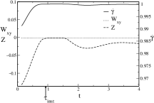
(d) $\dot{\gamma}=7.0$, eigenvector at $\log(k^{*}/\pi)=0.0$.

(e) $\dot{\gamma}=40.0$, eigenvector at $\log(k^{*}/\pi)=0.0$.

(f) $\dot{\gamma}=70.0$, eigenvector at $\log(k^{*}/\pi)=0.0$.

Figure 10: Type A instabilities in a type I system: time dependent dispersion relation (top) and eigenvector (bottom) in the uncoupled limit $\zeta\to\infty$ for $\phi=0.11$. The rheological model parameters all assume the experimental values of table 1. The thick line in Fig. 10(a) and the arrows in Figs. d,e,f denote the time at which the instability becomes measurable. The discontinuities in the first derivative of the eigenvector components result from a crossing of eigenvalues, discussed in the text.

.

(a) $\dot{\gamma}=2.0$, dispersion relation.

(b) $\dot{\gamma}=4.0$, dispersion relation.

(c) $\dot{\gamma}=35.0$, dispersion relation.

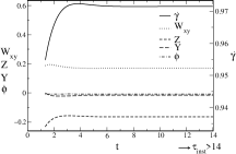
(d) $\dot{\gamma}=2.0$, eigenvector at $\log(k^{*}/\pi)=2.0$.

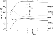
(e) $\dot{\gamma}=4.0$, eigenvector at $\log(k^{*}/\pi)=2.0$.

(f) $\dot{\gamma}=35.0$, eigenvector at $\log(k^{*}/\pi)=2.4$.

Figure 11: Type A instabilities in a type I system: time dependent dispersion relation (top) and eigenvector (bottom) for a coupled model in which all parameters assume the experimental values of table 1. The concentration $\phi=0.11$. The arrows in Figs. e,f show the time at which the instability first becomes measureable (the instability occurs beyond the time window of Fig. d). The discontinuities in the first derivative of the eigenvector components result from a crossing of eigenvalues, discussed in the text. The instability time $\tau_{\rm inst}$ occurs beyond the displayed time window for $\dot{\gamma}=2.0$.

.

(a) $\dot{\gamma}=0.01$, dispersion relation.

(b) $\dot{\gamma}=1.0$, dispersion relation.

(c) $\dot{\gamma}=10.0$, dispersion relation.

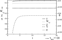
(d) $\dot{\gamma}=0.01$, eigenvector at $\log(k^{*}/\pi)=2.4$.

(e) $\dot{\gamma}=1.0$, eigenvector at $\log(k^{*}/\pi)=4.4$.

(f) $\dot{\gamma}=10.0$, eigenvector at $\log(k^{*}/\pi)=4.4$.

Figure 12: Type A instabilities (a,b,d,e) and type B instability (c,f) in a type II system: time dependent dispersion relation (top) and eigenvector (bottom) for a coupled model in which all parameters assume the experimental values of table 1, except $D$, which is reduced by a factor $10^{5}$. The concentration $\phi=0.11$. The arrows in Figs. e,f show the time at which the instability first becomes measureable (the instability occurs beyond the time window of Fig. d).

.

V.3 Results: coupled model

We now give startup results for the coupled model. Denoting the experimental DLS value of the diffusion coefficient $D$ (table 1) by $D_{\rm expt}$, figures 11 and 12 are for $D=D_{\rm expt}$ (type I system) and $D=10^{-5}D_{\rm expt}$ (type II system) respectively. The overall features of these dispersion relations are the same as for their time-independent counterparts (Figs. 4 and 6(b)). In particular there is, at any time, a well defined peak $k=k_{\rm peak}(t)$. This peak shifts along the $k$ axis in time. At $t=t_{0}$, when $\omega^{*}=0$ by definition, we numerically observe that $k_{\rm peak}=0$. However $k_{\rm peak}$ very quickly attains a value $k^{*}$ that is (practically) time-independent and well approximated by Eqn. 55 . In this way, the time-dependence of $k_{\rm peak}$ only occurs at early times $t\stackrel{{\scriptstyle>}}{{\scriptstyle\sim}}t_{0}$, for which the growth rate is insignificantly small. We argue, therefore, that we can choose the ultimate $k_{\rm peak}=k^{*}$ as the representative wavevector for the instability.

The time dependent eigenvector at this selected wavevector $k^{*}$ is also shown in figures 11 to 12. As noted above, the eigenvector encodes the extent to which separation occurs in each of different order parameters. Experimentally, polarised light scattering is sensitive to fluctuations in the micellar strain, while unpolarised light scattering measures fluctuations in the overall micellar concentration. In a forthcoming paper upc , we explicitly calculate the unstable startup static structure factor separately for polarised and unpolarised light scattering. In this paper, we restrict ourselves to the overall features on the instability that are deducible from the eigenvector.

For type I systems at all (unstable) shear rates (figures 11(d), 11(e) and 11(f)), and for type II systems at shear rates that are not too small (figures 12(e) and 12(f)), the eigenvector is dominated by the flow variables $\delta\dot{\gamma}$ and $\delta\underline{\underline{W}}$ as expected. In contrast, for the type II system at low shear rates (Fig. 12(d)) the eigenvector is dominated by concentration: here the instability is essentially CH demixing, triggered by flow. At higher shear rates, even in this type II system, the instability is basically mechanical. Note finally that concentration coupling affects the relative contributions of the shear ($W_{xy}$) and normal ($Z$) stresses. Recall that in the uncoupled limit, $\delta Z\gg\delta W_{xy}$. In this coupled case, the shear component can be comparable to $\delta Z$ (for moderate applied shear rate $\bar{\dot{\gamma}}$) or even larger than $\delta Z$ (low $\bar{\dot{\gamma}}$).

VI Conclusion

In this paper, we have studied the early-time kinetics of the shear banding instability in startup flows. Motivated by recent rheo-optical experimentsDecruppe et al. (2001) in which enhanced concentration fluctuations were observed in the flow/flow-gradient and flow/vorticity planes at the onset of instability, we performed a linear stability analysis for coupled fluctuations in shear rate, viscoelastic stress and concentration using the non-local Johnson-Segalman model and a two-fluid approach to concentration fluctuations.

We considered two flow histories. The first assumed an initial homogeneous state on the intrinsic constitutive curve. Using this, we defined the spinodal boundaries of the unstable region for slow shear rate sweeps. (Any real system can in practice shear band via metastable kinetics before the unstable region is reached. The analogous ambiguity occurs in the CH calculation for fluid-fluid demixing.) For the uncoupled limit of infinite drag between micelles and solvent at finite collective micellar diffusion constant $D$, fluctuations in the mechanical variables (shear rate and stress) decouple from concentration and are unstable when the intrinsic constitutive curve has negative slope, as expected; the concentration has its own CH instability for $D<0$.

For finite drag, fluctuations in the mechanical variables couple to those in concentration via the positive feedback mechanism of Helfand and Fredrickson, and the unstable region of what was the purely mechanical instability is broadened. In rapid upward stress sweep experiments, therefore, “top” jumping should in fact occur before the maxiumum in the intrinsic constitutive curve is reached. For given values of the coupling parameters, the degree of broadening increases with proximity to an underlying (zero shear) CH demixing instability. Accordingly, we classified systems into two types. Type I systems are far from a CH instability, and the mechanical instability is only slightly perturbed by concentration coupling. Type II systems are close to a CH instability. Type I systems, and type II systems at high shear rates, show instabilities that are predominantly mechanical (type A). Type II systems at low shear rates should show a CH instability perturbed by coupling to flow (type B).

We then discussed the dispersion relations for fluctuations about the unstable intrinsic constitutive curve. In the uncoupled limit, there is a broad plateau in the dispersion relation, with no selected length scale. Concentration coupling enhances the instability at short wavelengths thereby selecting a wavelength. However the typical growth rates predicted by these dispersion relations are larger than the rate at which the system can realistically be prepared on the intrinsic constitutive curve. We therefore explicitly considered shear startup quenches into the unstable region. We assumed that the startup flow can be decomposed into a homogeneous background state, evolving towards the intrinsic constitutive curve, with small fluctuations that (consistently with the above remarks) in general go unstable before the the intrinsic constitutive curve can be attained. The main features of the time independent dispersion relations for fluctuations about the intrinsic constitutive curve are nonetheless preserved: the mechanical instability shows length scale selection only when coupled to concentration. Our results for the time dependent eigenvector at this selected length scale confirmed our classification of instabilities into types A and B.

In the coupled model, for small values of the diffusion coefficient a second lobe of instability develops at high shear rates. This could clearly have dramatic consequences for any putative coexistence of low shear and high shear bands, since the high shear band could itself be unstable. Indeed, the high shear band is often seen to fluctuate strongly Britton and Callaghan (1999), or to break into smaller bands ler (a). However, in our model this high-shear instability is highly sensitive to choice of model parameters, and could be an unrealistic feature.

Our study was confined to fluctuations in the flow gradient direction, and to the qualitative features of the instability that can be gleaned from the time-dependent dispersion relations and eigenvectors. In a future paper, we will present results for the time-dependent unstable static structure factor in startup, for fluctuations in the entire flow/flow-gradient plane upc .

Acknowledgments We thank Paul Callaghan, Ron Larson, Sandra Lerouge, and Tom McLeish for interesting discussions and EPSRC GR/N 11735 for financial support; this work was supported in part by the National Science Foundation under Grant No.PHY99-07949.

References

- Cates (1990) M. E. Cates, J. Phys. Chem. 94, 371 (1990).
- Spenley and Cates (1994) N. A. Spenley and M. E. Cates, Macromolecules 27, 3850 (1994).
- Spenley et al. (1993) N. A. Spenley, M. E. Cates, and T. C. B. McLeish, Phys. Rev. Lett. 71, 939 (1993).
- Yerushalmi et al. (1970) J. Yerushalmi, S. Katz, and R. Shinnar, Chemical Engineering Science 25, 1891 (1970).
- Olmsted et al. (2000) P. D. Olmsted, O. Radulescu, and C.-Y. D. Lu, J. Rheology 44, 257 (2000).
- Lu et al. (2000) C.-Y. D. Lu, P. D. Olmsted, and R. C. Ball, Phys. Rev. Lett. 84, 642 (2000).
- Olmsted and Lu (1997) P. D. Olmsted and C.-Y. D. Lu, Phys. Rev. E56, 55 (1997).
- Olmsted and Goldbart (1992) P. D. Olmsted and P. M. Goldbart, Phys. Rev. A46, 4966 (1992).
- Pearson (1994) J. R. A. Pearson, J. Rheol. 38, 309 (1994).
- Yuan (1999) X. F. Yuan, Europhys. Lett. 46, 542 (1999).
- Spenley et al. (1996) N. A. Spenley, X. F. Yuan, and M. E. Cates, J. Phys. II (France) 6, 551 (1996).
- Berret et al. (1994a) J. F. Berret, D. C. Roux, and G. Porte, J. Phys. II (France) 4, 1261 (1994a).
- Callaghan et al. (1996) P. T. Callaghan, M. E. Cates, C. J. Rofe, and J. B. A. F. Smeulders, J. Phys. II (France) 6, 375 (1996).
- Grand et al. (1997) C. Grand, J. Arrault, and M. E. Cates, J. Phys. II (France) 7, 1071 (1997).
- Mair and Callaghan (1996a) R. W. Mair and P. T. Callaghan, Europhys. Lett. 36, 719 (1996a).
- Mair and Callaghan (1996b) R. W. Mair and P. T. Callaghan, Europhysics Letters 65, 241 (1996b).
- Britton and Callaghan (1997) M. M. Britton and P. T. Callaghan, Phys. Rev. Lett. 78, 4930 (1997).
- Berret et al. (1994b) J. F. Berret, D. C. Roux, G. Porte, and P. Lindner, Europhys. Lett. 25, 521 (1994b).
- Schmitt et al. (1994) V. Schmitt, F. Lequeux, A. Pousse, and D. Roux, Langmuir 10, 955 (1994).
- Cappelaere et al. (1997) E. Cappelaere, J. F. Berret, J. P. Decruppe, R. Cressely, and P. Lindner, Phys. Rev. E 56, 1869 (1997).
- Berret et al. (1998) J. F. Berret, D. C. Roux, and P. Lindner, European Physical Journal B 5, 67 (1998).
- Rehage and Hoffmann (1991) H. Rehage and H. Hoffmann, Mol. Phys. 74, 933 (1991).
- Decruppe et al. (1995) J. P. Decruppe, R. Cressely, R. Makhloufi, and E. Cappelaere, Coll. Polym. Sci. 273, 346 (1995).
- Makhloufi et al. (1995) R. Makhloufi, J. P. Decruppe, A. Aitali, and R. Cressely, Europhys. Lett. 32, 253 (1995).
- Decruppe et al. (1997) J. P. Decruppe, E. Cappelaere, and R. Cressely, J. Phys. II (France) 7, 257 (1997).
- Berret et al. (1997) J. F. Berret, G. Porte, and J. P. Decruppe, Phys. Rev. E 55, 1668 (1997).
- Fischer and Callaghan (2001) E. Fischer and P. T. Callaghan, Phys. Rev. E 6401, 1501 (2001).
- Fischer and Callaghan (2000) E. Fischer and P. T. Callaghan, Europhys. Lett. 50, 803 (2000).
- Berret (1997) J. F. Berret, Langmuir 13, 2227 (1997).
- Lerouge et al. (1998) S. Lerouge, J. P. Decruppe, and C. Humbert, Phys. Rev. Lett. 81, 5457 (1998).
- Decruppe et al. (2001) J. P. Decruppe, S. Lerouge, and J. F. Berret, Phys. Rev. E 6302, 2501 (2001).
- Lerouge et al. (2000) S. Lerouge, J. P. Decruppe, and J. F. Berret, Langmuir 16, 6464 (2000).
- Berret and Porte (1999) J. F. Berret and G. Porte, Phys. Rev. E 60, 4268 (1999).
- Helfand and Fredrickson (1989) E. Helfand and G. H. Fredrickson, Phys. Rev. Lett. 62, 2468 (1989).
- Schmitt et al. (1995) V. Schmitt, C. M. Marques, and F. Lequeux, Phys. Rev. E52, 4009 (1995).
- Brochard and de Gennes (1977) F. Brochard and P.-G. de Gennes, Macromolecules 10, 1157 (1977).
- Doi and Onuki (1992) M. Doi and A. Onuki, J. Phys. II (France) 2, 1631 (1992).
- Milner (1993) S. T. Milner, Phys. Rev. E48, 3674 (1993).
- Wu et al. (1991) X. L. Wu, D. J. Pine, and P. K. Dixon, Phys. Rev. Lett. 66, 2408 (1991).
- Clarke and McLeish (1998) N. Clarke and T. C. B. McLeish, Phys. Rev. E 57, R3731 (1998).
- Beris and Mavrantzas (1994) A. N. Beris and V. G. Mavrantzas, J. Rheol. 38, 1235 (1994).
- Sun et al. (1997) T. Sun, A. C. Balazs, and D. Jasnow, Phys. Rev. E 55, R6344 (1997).
- Tanaka (1996) H. Tanaka, Phys. Rev. Lett. 76, 787 (1996).
- Johnson and Segalman (1977) M. Johnson and D. Segalman, J. Non-Newt. Fl. Mech 2, 255 (1977).
- Milner (1991) S. T. Milner, Phys. Rev. Lett. 66, 1477 (1991).
- de Gennes (1976) P.-G. de Gennes, Macromolecules 9, 587 (1976).
- Brochard (1983) F. Brochard, J.Phys. (Paris) 44, 39 (1983).
- (48) S M Fielding and P D Olmsted. Submitted to Physical Review Letters.
- Onuki (1989) A. Onuki, Phys. Rev. Lett. 62, 2472 (1989).
- de Gennes (1975) P. G. de Gennes, Scaling Concepts in Polymer Physics (Cornell, Ithaca, 1975).
- neg (a) The criterion for neglecting the relative inertial terms when considering a fluctuation of rate and wavevector about a state of uniform shear rate is .
- Dhont (1999) J. K. G. Dhont, Phys. Rev. E 60, 4534 (1999).
- ler (a) S Lerouge. PhD Thesis, University of Metz, 2000.
- Candau et al. (1985) S. J. Candau, E. Hirsch, and R. Zana, J. Colloid Interface Sci. 105, 521 (1985).
- Radulescu and Olmsted (2000) O. Radulescu and P. D. Olmsted, J. Non-Newt. Fl. Mech 91, 141 (2000).
- Radulescu and Olmsted (1999) O. Radulescu and P. D. Olmsted, Rheol. Acta 38, 606 (1999).
- (57) Before rescaling, , and had dimensions , , and . Correspondingly, the size and direction of the vector would have been different in different units, and any vector operations must be applied with caution.
- neg (b) Matrix 34 neglects , which amounts to assuming that the velocity convecting the micellar strain is and not . It also neglects the positive feedback between flow and concentration involving the elastic contribution to the free energy in Eqn. 17.
- ler (b) S Lerouge. Private communication.
- Onuki and Taniguchi (1997) A. Onuki and T. Taniguchi, J. Chem. Phys. 106, 5761 (1997).
- (61) There are rare cases of multiple positive branches but never, for any regime investigated, in the relevant window of time .
- (62) S M Fielding and P D Olmsted. In preparation.
- Britton and Callaghan (1999) M. M. Britton and P. T. Callaghan, European Physical Journal B 7, 237 (1999).