Predictability in the ETAS Model of Interacting Triggered Seismicity

Abstract

As part of an effort to develop a systematic methodology for earthquake forecasting, we use a simple model of seismicity based on interacting events which may trigger a cascade of earthquakes, known as the Epidemic-Type Aftershock Sequence model (ETAS). The ETAS model is constructed on a bare (unrenormalized) Omori law, the Gutenberg-Richter law and the idea that large events trigger more numerous aftershocks. For simplicity, we do not use the information on the spatial location of earthquakes and work only in the time domain. We demonstrate the essential role played by the cascade of triggered seismicity in controlling the rate of aftershock decay as well as the overall level of seismicity in the presence of a constant external seismicity source. We offer an analytical approach to account for the yet unobserved triggered seismicity adapted to the problem of forecasting future seismic rates at varying horizons from the present. Tests presented on synthetic catalogs validate strongly the importance of taking into account all the cascades of still unobserved triggered events in order to predict correctly the future level of seismicity beyond a few minutes. We find a strong predictability if one accepts to predict only a small fraction of the large-magnitude targets. Specifically, we find a prediction gain (defined as the ratio of the fraction of predicted events over the fraction of time in alarms) equal to 21 for a fraction of alarm of 1%, a target magnitude $M\geq 6$, an update time of 0.5 days between two predictions, and for realistic parameters of the ETAS model. However, the probability gains degrade fast when one attempts to predict a larger fraction of the targets. This is because a significant fraction of events remain uncorrelated from past seismicity. This delineates the fundamental limits underlying forecasting skills, stemming from an intrinsic stochastic component in these interacting triggered seismicity models. Quantitatively, the fundamental limits of predictability found here are only lower bounds of the true values corresponding to the full information on the spatial location of earthquakes.

HELMSTETTER and SORNETTE Predictability of Triggered Seismicity Agnès Helmstetter, Laboratoire de Géophysique Interne et Tectonophysique, Observatoire de Grenoble, Université Joseph Fourier, BP 53X, 38041 Grenoble Cedex, France. (e-mail: ahelmste@obs.ujf-grenoble.fr) Didier Sornette, Department of Earth and Space Sciences and Institute of Geophysics and Planetary Physics, University of California, Los Angeles, California and Laboratoire de Physique de la Matière Condensée, CNRS UMR 6622 and Université de Nice-Sophia Antipolis, Parc Valrose, 06108 Nice, France (e-mail: sornette@moho.ess.ucla.edu) Laboratoire de Géophysique Interne et Tectonophysique, Observatoire de Grenoble, Université Joseph Fourier, France Department of Earth and Space Sciences and Institute of Geophysics and Planetary Physics, University of California, Los Angeles, California 90095-1567 and Laboratoire de Physique de la Matière Condensée, CNRS UMR 6622 Université de Nice-Sophia Antipolis, Parc Valrose, 06108 Nice, France

1 Introduction

There are several well documented facts in seismicity: (1) spatial clustering of earthquakes at many scales, [e.g. Kagan and Knopoff, 1980] (2) the Gutenberg-Richter (GR) [Gutenberg and Richter, 1944] distribution of earthquake magnitudes and (3) clustering in time following large earthquakes, quantified by Omori’s $\approx 1/t^{p}$ law for aftershocks (with $p\approx 1$) [Omori, 1894]. However, there are some deviations from these empirical laws, and a significant variability in the parameters of these laws. The $b$-value of the GR law, the $p$ Omori exponent and the aftershock productivity are spatially and temporally variable [Utsu et al., 1995; Guo and Ogata, 1997]. Some alternative laws have also been proposed, such as a gamma law for the magnitude distribution [Kagan, 1999] or the stretched exponential for the temporal decay of the rate of aftershocks [Kisslinger, 1993].

However, these “laws” are only the beginning of a full model of seismic activity and earthquake triggering. In principle, if one could obtain a faithful representation (model) of the spatio-temporal organization of seismicity, one could use this model to develop algorithms for forecasting earthquakes. The ultimate quality of these forecasts would be limited by the quality of the model, the amount of data that can be used in the forecast and its reliability and precision, and the stochastic component of seismic activity. Here, we analyze a simple model of seismicity known as the Epidemic Type Aftershock Sequence model (ETAS) [Ogata, 1988, 1989] and we use it to test the fundamental limits of predictability of this class of models. We restrict our analysis to the time domain, that is, we neglect the information provided by the spatial location of earthquakes which could be used to constrain the correlation between events and would be expected to improve forecasting skills. Our results should thus give lower bounds of the achievable predictive skills. This exercise is rather constrained but turns out to provide meaningful and useful insights. Because our goal is to estimate the intrinsic limits of predictability in the ETAS model, independently of the additional errors coming from the uncertainty in the estimation of the ETAS parameters in real data, we consider only synthetic catalogs generated with the ETAS model. Thus, the only source of error of the prediction algorithms result from the stochasticity of the model.

Before presenting the model and developing the tools necessary for the prediction of future seismicity, we briefly summarize in the next section the available methods of earthquake forecasting based on past seismicity. In section 3, we present the model of interacting triggered seismicity used in our analysis. Section 4 develops the formal solution of the problem of forecasting future seismicity rates based on the knowledge of past seismicity quantified by a catalog of times of occurrences and magnitudes of earthquakes. Section 5 gives the results of an intensive series of tests, which quantify in several alternative ways the quality of forecasts (regression of predicted versus realized seismicity rate, error diagrams, probability gains, information-based binomial scores). Comparisons with the Poisson null-hypothesis give a very significant success rate. However, only a small fraction of the large-magnitude targets can be shown to be successfully predicted while the probability gain deteriorates rapidly when one attempts to predict a larger fraction of the targets. We provide a detailed discussion of these results and of the influence of the model parameters. Section 6 concludes.

2 A rapid tour of methods of earthquake forecasts based on past seismicity

All the algorithms that have been developed for the prediction of future large earthquakes based on past seismicity rely on their characterization either as witnesses or as actors. In other words, these algorithms assume that past seismicity is related in some way to the approach of a large scale rupture.

2.1 Pattern recognition (M8)

In their pioneering work, Keilis-Borok and Malinovskaya [1964] codified an observation of general increase in seismic activity depicted with the only measure, “pattern Sigma”, which is characterizing the trailing total sum of the source areas of the medium size earthquakes. Similar strict codifications of other seismicity patterns, such as a decrease of $b$-value, an increase in the rate of activity, an anomalous number of aftershocks, etc, have been proposed later and define the M8 algorithm of earthquake forecast (see [Keilis-Borok and Kossobokov, 1990a; Keilis-Borok and Soloviev, 2002] for useful reviews). In these algorithms, an alarm is defined when several precursory patterns are above a threshold calibrated in a training period. Predictions are updated periodically as new data become available. Most of the patterns used by this class of algorithms are reproduced by the model of triggered seismicity known as the ETAS (Epidemic Type Aftershock Sequence) model [see Sornette and Sornette, 1999; Helmstetter and Sornette, 2002; Helmstetter et al., 2003]. The prediction gain $G$ of the M8 algorithm, defined as the ratio between the fraction of predicted events over the fraction of time occupied by alarms, is usually in the range 3 to 10 (recall that a random predictor would give $G=1$ by definition). A preliminary forward test of the algorithm for the time period July 1991 to June 1995 performed no better than the null hypothesis using a reshuffling of the alarm windows [Kossobokov et al., 1997]. Later tests indicated however a confidence level of 92% for the prediction of $M7.5+$ earthquakes by the algorithm M8-MSc for real-time intermediate-term predictions in the Circum Pacific seismic belt, 1992-1997, and above 99% for the prediction of $M\geq 8$ earthquakes [Kossobokov et al., 1999]. We use the term confidence level as $1$ minus the probability of observing a predictability at least as good as what was actually observed, under the null hypothesis that everything is due to chance alone. As of July 2002, the scores (counted from the formal start of the global test initiated by this team since July 1991) are as follows: For $M8.0+$, 8 events occurred, 7 predicted by M8, 5 predicted by M8-MSc; for $M7.5+$, 25 events occurred, 15 predicted by M8 and 7 predicted by M8-MSc.

2.2 Short term forecast of aftershocks

Reasenberg and Jones [1989] and Wiemer [2000] have developed algorithms to predict the rate of aftershocks following major earthquakes. The rate of aftershocks of magnitude $m$ following an earthquake of magnitude $M$ is estimated by the expression

$$N_{M}(m)={k~{}10^{b(M-m)}\over(t+c)^{p}}~{},$$ (1)

where $b\approx 1$ is the $b$-value of the Gutenberg-Richter (GR) distribution. This approach neglects the contribution of seismicity prior to the mainshock, and does not take into account the specific times, locations and magnitudes of the aftershocks that have already occurred. In addition, this model (1) assumes arbitrarily that the rate of aftershocks increases with the magnitude $M$ of the mainshock as $\sim 10^{bM}$, which may not be correct. A careful measure of this scaling for the southern California seismicity gives a different scaling $\sim 10^{\alpha M}$ with $\alpha=0.8$ [Helmstetter, 2003]. Moreover, an analytical study of the ETAS model [Sornette and Helmstetter, 2002] shows that the case $\alpha\geq b$ leads to an explosive seismicity rate, which is unrealistic to describe the seismic activity.

2.3 Branching models

Simulations using branching models as a tool for predicting earthquake occurrence over large time horizons were proposed in Kagan [1973], and first implemented in Kagan and Knopoff [1977]. In a recent work, Kagan and Jackson [2000] use a variation of the ETAS model to estimate the rate of seismicity in the future but they neglect the seismicity that will be triggered between the present time and the horizon and which may dominate the future activity. Therefore, these predictions are only valid at very short times, when very few earthquakes have occurred between the present and the horizon.

To solve this problem and to extend the predictions further in time, Kagan and Jackson [2000] propose to use Monte-Carlo simulations to generate many possible scenarios of the future seismic activity. However, they do not use this method in their forecasting procedure. These Monte-Carlo simulations will be implemented in our tests, as we describe below. This method has already been tested by Vere-Jones [1998] to predict a synthetic catalog generated using the ETAS model. Using a measure of the quality of seismicity forecasts in terms of mean information gain per unit time, he obtains scores usually worse than the Poisson method. We use below the same class of model and implement a procedure taking into account the cascade of triggering. We find, in contrast with the claim of Vere-Jones [1998], a very strong probability gain. We explain in section 5.6 the origin of this discrepancy, which can be attributed to the use of different measures for the quality of predictions.

In [Helmstetter et al., 2003], the forecasting skills of algorithms based on three functions of the current and past seismicity (above a magnitude threshold) measured in a sliding window of 100 events have been compared. The functions are (i) the maximum magnitude $M_{max}$ of the 100 events in that window, (ii) the Gutenberg-Richter $b$-value measured on these 100 events by the standard Hill maximum likelihood estimator and (iii) the seismicity rate $\lambda$ defined as the inverse of the duration of the window. For each function, an alarm was declared for the target of an earthquake of magnitude larger than $6$ when the function is either larger (for $M_{max}$ and $\lambda$) or smaller (for $b$) than a threshold. These functions $M_{max}$, $b$ and $\lambda$ are similar and in some cases identical to precursors and predictors that have been studied by other authors. Helmstetter et al. [2003] found that these three predictors are considerably better than those obtained for a random prediction, with the prediction based on the seismicity rate $\lambda$ being by far the best. This is a logical consequence of the model of interacting triggered seismicity used in Helmstetter et al. [2003] and also in the present work, in which any relevant physical observable is a function of the seismicity rate. At least in the class of interacting triggered seismicity, the largest possible amount of information is recovered by targeting the seismicity rate. All other targets are derived from it as linear or non-linear transformations of it. Our present study refines and extends the preliminary tests of Helmstetter et al. [2003] by using a full model of seismicity rather than the coarse-grained measure $\lambda$. We note also that the forecasting methods of Rundle et al. [2001; 2002] are based on a calculation of the coarse-grained seismicity above a small magnitude threshold, which is then projected into the future.

3 The model of triggered seismicity

The parametric form that defines the ETAS model used in this paper was formulated by Ogata [1985, 1987, 1988]. See [Ogata, 1999] and [Helmstetter and Sornette, 2002a] for reviews of its origins, a description of the different versions of the model and of its applications to model or predict seismic activity. It is important to stress that the ETAS model is not only a model of aftershock sequences as the acronym ETAS (Epidemic-Type Aftershock Sequence) would make one to believe but is fundamentally a model of triggered interacting seismicity.

In addition to the strict definition of the ETAS model used by Ogata [1985, 1987, 1988, 1989, 1999], there were and still are a variety of alternative parametric forms of the extended “mutually exciting point processes” with marks (that is, magnitudes) introduced by Hawkes [1971, 1972], which have been applied to earthquakes, including Kagan and Knopoff [1987]; Kagan [1991] and Lomnitz [1974]. Kagan and Knopoff [1987] differs from Ogata [1985, 1987, 1988] in replacing the role played by the parameter $c$ in the modified Omori law (1) by an abrupt cut-off which models the duration of the mainshock. They think that a non-zero value of $c$ is merely the artifact of the missing events immediately after the mainshock In contrast, based on the observation of the records of seismic waves, Utsu [1970, 1992] considers that the parameter $c$ is not merely due to such artifact but also possesses some physical meaning. The analysis of Helmstetter and Sornette [2002a] shows that the choice of a non-zero $c$ value [Ogata, 1988] or an abrupt cut-off [Kagan and Knopoff, 1987] does not lead to any detectable differences in simulated catalogs at time scales beyond $c$ (which is usually very small). Thus, from the point of view of the collective behavior of the model, both formulations lead to essentially indistinguishable catalogs and statistical properties. Lomnitz [1974]’s model (“Klondike model”) was also directly inspired by Hawkes [1971] and is similar to the ETAS model, but assumes different parametric forms: in particular, the number of triggered events is taken proportional to the magnitude, not the exponential of the magnitude. Kagan and Jackson [2000] also use a formulation of the same class but with a more complex specification of the time, space and magnitude dependence of the triggering process and propagator.

3.1 Definition of the ETAS model

The ETAS model of triggered seismicity is defined as follows [Ogata, 1985; 1987; 1988; 1989; 1992; 1999]. We assume that a given event (the “mother”) of magnitude $m_{i}\geq m_{0}$ occurring at time $t_{i}$ and position $\vec{r}_{i}$ gives birth to other events (“daughters”) in the time interval between $t$ and $t+dt$ and at point $\vec{r}\pm\vec{d}r$ at the rate

$$\phi_{m_{i}}(t-t_{i},\vec{r}-\vec{r}_{i})=\rho(m_{i})~{}\Phi(t-t_{i})~{}\Phi(\vec{r}-\vec{r}_{i})~{}.$$ (2)

$\Phi(t)$ is the direct Omori law normalized to $1$

$$\Phi(t)={\theta~{}c^{\theta}\over(t+c)^{1+\theta}}~{}H(t)~{},$$ (3)

where $\theta>0$, $H(t)$ is the Heaviside function, and $c$ is a regularizing time scale that ensures that the seismicity rate remains finite close to the mainshock.

$\Phi(\vec{r}-\vec{r}_{i})$ is a normalized spatial “jump” distribution from the mother to each of her daughter, which quantifies the probability for a daughter to be triggered at a distance $|\vec{r}-\vec{r}_{i}|$ from the mother, taking into account the spatial dependence of the stress induced by an earthquake.

$\rho(m)$ gives the total number of aftershocks triggered directly by an event of magnitude $m$

$$\rho(m)=k~{}10^{\alpha(m-m_{0})}~{},$$ (4)

where $m_{0}$ is a lower bound magnitude below which no daughter is triggered. The adjective “direct” refers to the events of the first generation triggered in first-order lineage from the mother event. The formulation of (3) and (4) is originally due to Utsu [1970].

The model is complemented by the Gutenberg-Richter (GR) law which states that each earthquake has a magnitude chosen according to the density distribution

$$P(m)=b~{}\ln(10)~{}10^{-b(m-m_{0})}~{}.$$ (5)

$P(m)$ is normalized: $\int_{m_{0}}^{\infty}~{}P(m)~{}dm=1$. When magnitudes are translated into energies, the GR law becomes the (power law) Pareto law. See [Ogata, 1989; 1992; 1999; Guo and Ogata, 1997; Helmstetter and Sornette, 2002a] for a discussion of the values of the ETAS parameters $c$, $\alpha$, $\theta$, $K$ and $b$ in real seismicity. Note however that we have reasons to think that previous inversions of the ETAS parameters in real data are unreliable due to lack of concern for the unobserved seismicity below the completeness threshold. We are presently working on methods to address this question.

In this first investigation, we limit ourselves to the time domain, studying time series of past seismicity summed over an overall spatial region, without taking into account information on earthquake locations. This amounts to integrating the local Omori law (2) over the whole space. In the following, we will thus use the integrated form of the local Omori law (2) given by

$$\phi_{m_{i}}(t-t_{i})=\int\limits_{r}\phi_{m_{i}}(t-t_{i},\vec{r}-\vec{r}_{i})~{}dr=\rho(m_{i})~{}\Phi(t-t_{i})~{}.$$ (6)

The complete model with both spatial and temporal dependence (2) has been studied in [Helmstetter and Sornette, 2002b] to derive the joint probability distribution of the times and locations of aftershocks including the whole cascade of secondary and later-generations aftershocks. When integrating the rate of aftershocks calculated for the spatio-temporal ETAS model over the whole space, we recover the results used in this paper for the temporal ETAS model.

We stress that not taking into account the spatial positions of the earthquakes is not saying that earthquakes occur at the same position. The synthetic catalogs we generate in space and time are similar to real catalogs and our procedure just neglects the information on space. Clearly, this is not what a full prediction method should do and it is clear that not using the information on the location of earthquakes will underestimate (sometimes grossly) the predictive skills that could be achieved with a full spatio-temporal treatment. However, the problem is sufficiently complex that we find it useful to go through this first step and develop the relevant concepts and first tests using only information on seismic time sequences.

3.2 Definition of the average branching ratio $n$

The key parameter of model (2) is the average number (or “branching ratio”) $n$ of daughter-earthquakes created per mother-event. This average is performed over time and over all possible mother magnitudes. This average branching ratio $n$ is a finite value for $\theta>0$ and for $\alpha<b$, equal to

$$n\equiv\int\limits_{0}^{\infty}dt\int\limits_{m_{0}}^{\infty}~{}P(m)~{}\rho(m)~{}\Phi(t)~{}dm={kb\over b-\alpha}.$$ (7)

The normal regime corresponds to the subcritical case $n<1$ for which the seismicity rate decays after a mainshock to a constant level (in the case of a steady-state source) with fluctuations in the seismic rate.

Since $n$ is defined as the average over all mainshock magnitudes of the mean number of events triggered by a mainshock, the branching ratio does not give the number of daughters of a given earthquake, because this number also depends on the specific value of its magnitude as shown by (4). As an example, take $\alpha=0.8$, $b=1$, $m_{0}=0$ and $n=1$. Then, a mainshock of magnitude $M=7$ will have on average 80000 direct aftershocks, compared to only 2000 direct aftershocks for an earthquake of magnitude $M=5$ and less than 0.2 aftershocks for an earthquake of magnitude $M=0$.

The branching ratio defined by (7) is the key parameter of the ETAS model, which controls the different regimes of seismic activity. There are two observable interpretations for this parameter [Helmstetter and Sornette, 2003]. The branching ratio can be defined as the ratio of triggered events over total seismicity when looking at catalog of seismicity at large scale. The branching ratio is also equal to the ratio of the number of secondary and later-generations aftershocks over the total number of aftershocks within a single aftershock sequence.

4 Formal solution of the earthquake forecast problem in the ETAS model

Having stressed the importance of the indirect triggered seismicity in determining both the overall level of seismicity and its decay law, we now formulate the task of earthquake forecast within this model of triggered seismicity restricted to the time domain. In this paper, we do not address the delicate issue related to the fact that not all earthquakes are observable or observed. Indeed, calibrations of the ETAS parameters using the magnitude cut-offs dictated by the requirement of seismic catalog completeness rather than by the physics of triggered seismicity may lead to misleading results, as unobserved events may play a significant role (in their sheer number) in triggering observable seismicity. To our knowledge, all previous calibrations of real seismic catalogs have bypassed this problem, which will be studied using a technique derived from our renormalized Omori law in a subsequent paper.

We first summarize the single source prediction problem, which has been studied previously by Helmstetter and Sornette [2002a]. We then consider the complete prediction problem and derive analytically the solution for the future seismicity rate triggered by all past event and by a constant external loading.

4.1 Formulation of the global seismicity rate and renormalized Omori’s law

We define the “bare propagator” $\phi(t)$ of the seismicity as the integral of (2) over all magnitudes

$$\phi(t)=\int\limits_{m_{0}}^{\infty}P(m)~{}\phi_{m}(t)~{}dm=n\Phi(t)~{},$$ (8)

which is normalized to $n$ since $\Phi(t)$ is normalized to $1$. The meaning of the adjective “bare” will become clear below, when we demonstrate that cascades of triggered events renormalize $\phi(t)$ into an effective (“renormalized” or “dressed”) propagator $K(t)$. This terminology is borrowed from statistical and condensed-matter physics which deal with physical phenomena occurring at multiple scales in which similar cascades of fluctuations lead to a renormalization of “bare” into “dressed” properties when going from small to large scales. See also [Sornette and Sornette, 1999; Helmstetter and Sornette, 2002a] where this terminology was introduced in the present context.

The total seismicity rate $\lambda(t)$ at time $t$ is given by the sum of an “external” source $s(t)$ and the aftershocks triggered by all previous events

$$\lambda(t)=s(t)+\sum_{i|t_{i}\leq t}\phi_{m_{i}}(t-t_{i})~{},$$ (9)

where $\phi_{m_{i}}(t-t_{i})$ is defined by (2). Here, “external” source refers to the concept that $s(t)$ is the rate of earthquakes not triggered by other previous earthquakes. This rate acts as a driving force ensuring that the seismicity does not vanish and models the effect of the external tectonic forcing.

Taking the ensemble average of (9) over many possible realizations of the seismicity (or equivalently taking the mathematical expectation), we obtain the following equation for the first moment or statistical average $N(t)$ of $\lambda(t)$ [Sornette and Sornette, 1999; Helmstetter and Sornette, 2002a]

$$N(t)=s(t)+\int\limits_{-\infty}^{t}~{}\phi(t-\tau)~{}N(\tau)~{}d\tau.$$ (10)

The average seismicity rate is the solution of this self-consistent integral equation, which embodies the fact that each event may start a sequence of events which can themselves trigger secondary events and so on. The cumulative effect of all the possible branching paths of activity gives rise to the net seismic activity $N(t)$. Expression (10) states that the seismic activity at time $t$ is due to a possible external source $s(t)$ plus the sum over all past times $\tau$ of the total previous activities $N(\tau)$ that may trigger an event at time $t$ according to the bare Omori law $\phi(t-\tau)$.

The global rate of aftershocks including secondary and later-generations aftershocks triggered by a mainshock of magnitude $M$ occurring at $t=0$ is given by $\rho(M)K(t)/n$, where the renormalized Omori law $K(t)$ is obtained as a solution of (10) with the general source term $s(t)$ replaced by the Dirac function $\delta(t)$:

$$K(t)=\delta(t)+\int\limits_{0}^{t}~{}\phi(t-\tau)~{}K(\tau)~{}d\tau~{}.$$ (11)

The solution for $K(t)$ can be obtained as the following series [Helmstetter and Sornette, 2002a]

$$K(t)=\delta(t)+{1\over 1-n}~{}{{t^{*}}^{-\theta}\over t^{1-\theta}}~{}\sum_{k=0}^{k=\infty}~{}(-1)^{k}~{}{(t/t^{*})^{k\theta}\over\Gamma((k+1)\theta)}~{}.$$ (12)

The infinite sum expansion is valid for $t>c$, and $t^{*}$ is a characteristic time measuring the distance to the critical point $n=1$ defined by

$$t^{*}=c\Bigl{(}{n\Gamma(1-\theta)\over|1-n|}\Bigr{)}^{1/\theta}~{}.$$ (13)

$t^{*}$ is infinite for $n=1$ and becomes very small for $n\ll 1$. The leading behavior of $K(t)$ at short times reads

$$K(t)={1\over 1-n}~{}{1\over\Gamma(\theta)}~{}{{t^{*}}^{-\theta}\over t^{1-\theta}}~{},~{}~{}~{}~{}~{}~{}~{}{\rm for}~{}c<t<t^{*}~{},$$ (14)

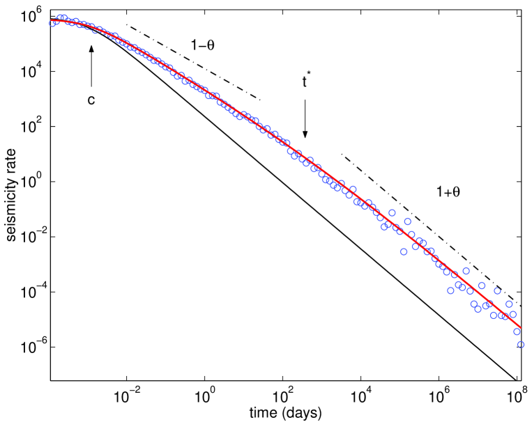
Figure 1: A realization of the ETAS model shows the seismicity rate (open circles) as a function of time after a large earthquake. This illustrates the differences between the realized seismicity rate $\lambda(t)$ (open circle), the average renormalized (or dressed) propagator $K(t)$ (gray line), and the local propagator $\Phi_{m}(t)$ (thin black line) . This aftershock sequence has been generated using the ETAS model with parameters $n=0.91$, $\alpha=0.5$, $b=1$, $\theta=0.2$, $m_{0}=0$ and $c=0.001$ day, starting from a mainshock of magnitude $M=8$ at time $t=0$. The global aftershock rate is significantly higher than the direct (or first generation) aftershock rate, described by the local propagator $\Phi_{m}(t)$. The value of the branching ratio $n=0.915$ implies that about $91.5$% of aftershocks are triggered indirectly by the mainshock. The global aftershock rate $N(t)$ decreases on average according to the dressed propagator $K(t)\sim 1/t^{1-\theta}$ for $t<t^{*}$, which is significantly slower than the local propagator $\phi(t)\sim 1/t^{1+\theta}$. These two asymptotic power laws are shown as dotted-dashed lines with their slopes in the log-log plot corresponding respectively to the exponents $1-\theta$ and $1+\theta$.

showing that the effect of the cascade of secondary aftershocks renormalizes the bare Omori law $\Phi(t)\sim 1/t^{1+\theta}$ given by (3) into $K(t)\sim 1/t^{1-\theta}$, as illustrated by Figure 1.

Once the seismic response $K(t)$ to a single event is known, the complete average seismicity rate $N(t)$ triggered by an arbitrary source $s(t)$ can be obtained using the theorem of Green functions for linear equations with source terms [Morse and Feshbach, 1953]

$$N(t)=\int\limits_{-\infty}^{t}~{}s(\tau)~{}K(t-\tau)~{}d\tau.$$ (15)

Expression (15) provides the general solution of (10).

4.2 The multiple source prediction problem

We assume that seismicity which occurred in the past until the “present” time $u$, and which does trigger future events, is observable. The seismic catalog consists of a list of entries $\{(t_{i},m_{i}),t_{i}<u\}$ giving the times $t_{i}$ of occurrence of the earthquakes and their magnitude $m_{i}$. Our goal is to set up the best possible predictor for the seismicity rate for the future from time $u$ to time $t>u$, based on the knowledge of this catalog $\{(t_{i},m_{i}),t_{i}<u\}$. The time difference $t-u$ is called the horizon. In the ETAS model studied here, magnitudes are determined independently of the seismic rate, according to the GR distribution. Therefore, the sole meaningful target for prediction is the seismic rate. Once its forecast is issued, the prediction of strong earthquakes is obtained by combining the GR law with the forecasted seismic rate.

The average seismicity rate $N(t)$ at time $t>u$ in the future is made of two contributions:

• the external source of seismicity of intensity $\mu$ at time $t$ plus the external source of seismicity that occurred between $u$ and $t$ and their following aftershocks that may trigger an event at time $t$;

• the earthquakes that have occurred in the past at times $t_{i}<u$ and all the events they triggered between $u$ and $t$ and their following aftershocks that may trigger an event at time $t$.

We now examine each contribution in turn.

4.2.1 Seismicity at times $t>u$ triggered by a constant source $\mu$ active from $u$ to $t$

Using the external seismicity source $\mu$ to forecast the seismicity in the future would underestimate the seismicity rate because it does not take into account the aftershocks of the external loading. On the contrary, using the “renormalized” seismicity rate $\mu/(1-n)$ derived in [Helmstetter and Sornette, 2003] would overestimate the seismicity rate because the earthquakes that were triggered before time $u$ by the external source would be counted twice, since they are registered in the catalog up to time $u$. The correct procedure is therefore to evaluate the rate of seismicity triggered by a constant source $\mu$ starting at time $u$ to remove the influence of earthquakes that have been recorded at times less than $u$, whose influence for times larger than $u$ is examined later.

The response $K_{\mu}(t)$ of the seismicity to a constant source term $\mu$ starting at time $u$ is obtained using (15) as

$$K_{\mu,u}(t)=\mu~{}\int\limits_{u^{+}}^{t}~{}[K(t-\tau)-\delta(t-\tau)]~{}d\tau=\mu~{}{\cal K}(t-u)~{},$$ (16)

where ${\cal K}(t)$ is the integral of $K(t)-\delta(t)$ given by (12) from the lower bound $u$ excluded (noted $u^{+}$) to $t$. This yields

$${\cal K}(t)={1\over 1-n}~{}\Bigl{(}{t\over t^{*}}\Bigr{)}^{\theta}~{}\sum_{k=0}^{k=\infty}(-1)^{k}~{}{(t/t^{*})^{k\theta}\over\Gamma((k+1)\theta+1)}~{}.$$ (17)

For times larger that $t\gg t^{*}$, $K_{\mu}(t)$ reaches the asymptotic value $K_{\mu}={\mu\over 1-n}$. Expression (16) takes care of both the external source seismicity of intensity $\mu$ at time $t$ and of its aftershocks and their following aftershocks from time $u$ to $t$ that may trigger events at time $t$.

4.2.2 Hypermetropic renormalized propagator

We now turn to the effect counted from time $u$ of the past known events prior to time $u$ on future $t>u$ seismicity, taking into account the direct, secondary and all later-generation aftershocks of each earthquakes that have occurred in the past at times $t_{i}<u$. Since the ETAS model is linear in the rate variable, we consider first the problem of a single past earthquake at time $t_{i}<u$ and will then sum over all past earthquakes.

A first approach for estimating the seismicity at $t>u$ due to event $i$ that occurred at time $t_{i}<u$ is to use the bare propagators $\Phi(t-t_{i})$, as done e.g. by Kagan and Jackson [2000]. This extrapolation leads to an underestimation of the seismicity rate in the future because it does not take into account the secondary aftershocks. This is quite a bad approximation when $n$ is not very small, and especially for $n>0.5$, since the secondary aftershocks are then more numerous than direct aftershocks.

An alternative would be to express the seismicity at $t>u$ due to an earthquake that occurred at $t_{i}<u$ by the global propagator $K(t-t_{i})$. However, this approach would overestimate the seismicity rate at time $t$ because of double counting. Indeed, $K(t-t_{i})$ takes into account the effect of all events triggered by event $i$, including those denoted $j$’s that occurred at times $t_{i}<t_{j}<u$ and which are directly observable and counted in the catalog. Thus, using $K(t-t_{i})$ takes into account these events $j$, that are themselves part of the sum of contributions over all events in the catalog.

The correct procedure is to calculate the seismicity at $t>u$ due to event $i$ by including all the seismicity that it triggered only after time $u$. This defines what we term the “hypermetropic renormalized propagator” $K_{u}^{*}(t-t_{i})$. It is “renormalized” because it takes into account secondary and all subsequent aftershocks. It is “hypermetropic” because this counting of triggered seismicity starts only after time $u$ such that this propagator is oblivious to all the seismicity triggered by event $i$ at short times from $t_{i}$ to $u$.

We now apply these concepts to estimate the seismicity triggered directly or indirectly by a mainshock with magnitude $M$ that occurred in the past at time $t_{i}$ while removing the influence of the triggered events $j$ occurring between $t_{i}$ and $u$. This gives the rate

$$S_{M}(t)={\rho(M)\over n}~{}K_{u}^{*}(t-t_{i})~{},$$ (18)

where the hypermetropic renormalized propagator $K_{u}^{*}$ is given by

$$K_{u}^{*}(t)=\int\limits_{u}^{t}~{}\phi(\tau)~{}K(t-\tau)~{}d\tau~{}.$$ (19)

$K_{u}^{*}(t)$ defined by (19) recovers the bare propagator $\Phi(t)$ for $t\approx u$, i.e., when the rate of direct aftershocks dominates the rate of secondary aftershocks triggered at time $t>u$. Indeed, taking the limit of (19) for $u\to t$ gives

$$K_{u\to t}^{*}(t) = \int\limits_{u\to t}^{t}~{}\phi(\tau)~{}K(t-\tau)~{}d\tau$$ (20)

$$= \int\limits_{u\to t}^{t}~{}\phi(\tau)~{}\delta(t-\tau)~{}d\tau=\phi(t)~{}.$$

This result simply means that the forecasting of future seismicity in the near future is mostly dominated by the sum of the direct Omori laws of all past events. This limit recovers procedures used by Kagan and Jackson [2000].

In the other limit, $u\approx t_{i}$, i.e., for an event that occurred at a time $t_{i}$ just before the present $u$, $K_{u}^{*}(t)$ recovers the dressed propagator $K(t)$ (up to a Dirac function) since there are no other registered events between $t_{i}$ and $t$ and all the seismicity triggered by event $i$ must be counted. Using equation (11), this gives

$$K_{u\to 0}^{*}(t)=\int\limits_{u\to 0}^{t}~{}\phi(\tau)~{}K(t-\tau)~{}d\tau=K(t)-\delta(t)~{}.$$ (21)

Using again (11), we can rewrite (19) as

$$K_{u}^{*}(t)=K(t)-\int\limits_{0}^{u}K(t-\tau)~{}\phi(\tau)~{}d\tau~{}.$$ (22)

Putting (12) in (19) we obtain for $t\geq c$

$$K_{u}^{*}(t) = {\theta\over\Gamma(\theta)~{}\Gamma(1-\theta)}~{}\int\limits_{0}^{t-u}~{}{1\over(t-x+c)^{1+\theta}}~{}{1\over x^{1-\theta}}~{}$$ (23)

$$\sum_{k=0}^{\infty}\Bigl{[}(-1)^{k}~{}{(x/t^{*})^{k\theta}\over\Gamma((k+1)\theta)}\Bigr{]}~{}dx~{},$$

where $x=t-\tau$.

We present below useful asymptotics and approximations of $K_{u}^{*}(t)$.

• Hypermetropic renormalized propagator for $t\ll t^{*}$

  Putting the asymptotic expansion of $K(t)$ for $t<t^{*}$ (14) in (19) we obtain for $t\gg c$ and $t>u$

  $$K^{*}_{u<t<t^{*}}(t)={1\over\Gamma(\theta)~{}\Gamma(1-\theta)}~{}{(t+c-u)^{\theta}\over(u+c)^{\theta}~{}(t+c)}~{},$$ (24)

  which recovers $K(t)$ for $u=0$.

• Hypermetropic renormalized propagator for $t\gg u$

  In the regime $t\gg u$, we can rewrite (22) as

  $$K_{u}^{*}(t) \approx K(t)-K(t)~{}\int_{0}^{u}~{}\phi(\tau)~{}d\tau$$ (25)

  $$\approx K(t)\Bigl{(}1-n\Bigl{(}1-{c^{\theta}\over(u+c)^{\theta}}\Bigr{)}\Bigr{)}$$

• Hypermetropic renormalized propagator for $t\approx u$

  In the regime $t\approx u$ and $t-u\gg c$, we can rewrite (19) as

  $$K_{u}^{*}(t) \approx \phi(t)~{}\int\limits_{u}^{t}~{}K(t-\tau)~{}d\tau$$ (26)

  $$\approx \phi(t)~{}({\cal K}(t-u)+1)~{},$$

  where ${\cal K}(t)$ is the integral of $K(t)-\delta(t)$ given by (17). The additional $1$ in (26) comes from the Dirac $\delta(t)$ in the expression (11) of $K(t)$.

We have performed numerical simulations of the ETAS model to test our predictions on the hypermetropic renormalized propagator $K_{u}^{*}(t)$ (19,23).

For the unrealistic case where $\alpha=0$, i.e., all events trigger the same number of aftershocks whatever their magnitude, the simulations show a very good agreement (not shown) between the results obtained by averaging over 1000 synthetic catalogs and the theoretical prediction (19,23).

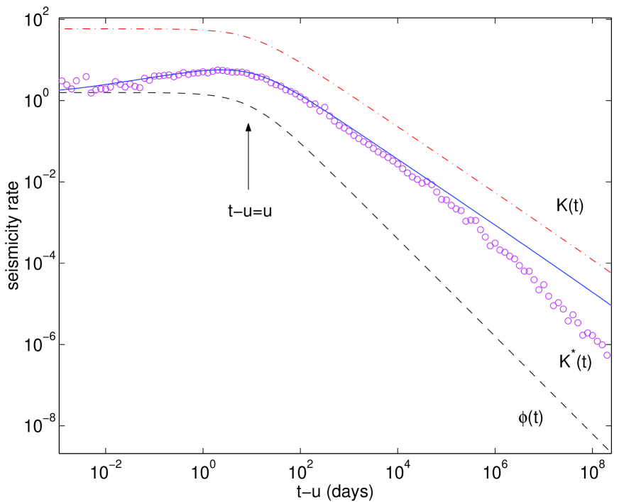
Figure 2: Seismicity rate (hypermetropic renormalized propagator) following a large event that happened at time $t=0$, removing the influence of aftershocks that were triggered in the past $0<t_{i}<u$ with $u=10$ days. We have averaged over 1000 simulations starting at time $u=10$ days after a large event of magnitude $m=6$, using the parameters $n=1$, $c=0.001$ day, $\theta=0.2$ and $\alpha=0.5$. There is a very good agreement between the realized hypermetropic seismicity rate (open circles) and $K_{u}^{*}(t)$ predicted by (19) and shown as the continuous line up to times $t-u\sim 10^{3}~{}u$. At large times, there is clear deviation between our numerical average of realized seismicity and the hypermetropic seismicity rate $K_{u}^{*}(t)$ due to a combination of a survival bias and large fluctuations in the numerics.

Figure 2 compares the numerical simulations with our theoretical prediction for more realistic parameters $\alpha=0.5$ with $n=1$, $c=0.001$ day, $\theta=0.2$ and $\mu=0$. In the simulations, we construct 1,000 synthetic catalogs, each generated by a large event that happened at time $t=0$. The numerical hypermetropic renormalized propagator or seismic activity $K_{u}^{*}(t)$ is obtained by removing for each catalog the influence of aftershocks that were triggered in the past $0<t_{i}<u$ where the present is taken equal to $u=10$ days and then by averaging over the 1,000 catalogs. It can then be compared with the theoretical prediction (19,23). Figure 2 exhibits a very good agreement between the realized hypermetropic seismicity rate (open circles) and $K_{u}^{*}(t)$ predicted by (19) and shown as the continuous line up to times $t-u\sim 10^{3}~{}u$. The hypermetropic renormalized propagator $K_{u}^{*}(t)$ is significantly larger than the bare Omori law $\Phi(t)$ but smaller than the renormalized propagator $K(t)$ as expected. Note that $K_{u}^{*}(t)$ first increases with the horizon $t-u$ up to horizons of the order of $u$ and then crosses over to a decay law $K_{u}^{*}(t)\sim 1/t^{1-\theta}$ parallel to the dressed propagator $K(t)$. At large times however, one can observe a new effect in the clear deviation between our numerical average of the realized seismicity and the hypermetropic seismicity rate $K_{u}^{*}(t)$. This deviation pertains to a large deviation regime and is due to a combination of a survival bias and large fluctuations in the numerics. For the larger value $\alpha=0.8$, which may be more relevant for seismicity, the deviation between the simulated seismicity rate and the prediction is even larger. Indeed, for $\alpha\geq 1/2$, Helmstetter et al. [2003] have shown that the distribution of first-generation seismicity rate is a power law with exponent less than or equal to $2$, implying that its variance is ill-defined (or mathematically infinite). Thus, averages converge slowly, all the more so at long times where average rates are small and fluctuations are huge. Another way to state the problem is that, in this regime $\alpha\geq 1/2$, the average seismicity may be a poor estimation of the typical or most probable seismicity. Such effect can be taken into account approximately by taking into account the coupling between the fluctuations of the local rates and the realized magnitudes of earthquakes at a coarse-grained level of description [Helmstetter et al., 2003]. A detailed analytical quantification of this effect for $K(t)$ (already discussed semi-quantitatively in [Helmstetter et al., 2003]) and for $K_{u}^{*}(t)$, with an emphasis on the difference between the average, the most probable and different quantiles of the distribution of seismic rates, will be reported elsewhere.

Since we are aiming at predicting single catalogs, we shall resort below to robust numerical estimations of $K(t)$ and $K_{u}^{*}(t)$ obtained by generating numerically many seismic catalogs based on the known seismicity up to time $u$. Each such catalog synthesized for times $t>u$ constitutes a possible scenario for the future seismicity. Taking the average and calculating the median as well as different quantiles over many such scenarios provides the relevant predictions of future seismicity for a single typical catalog as well as its confidence intervals.

5 Forecast tests with the ETAS model

Because our goal is to estimate the intrinsic limits of predictability in the ETAS model, independently of the additional errors coming from the uncertainty in the estimation of the ETAS parameters in real data, we consider only synthetic catalogs generated with the ETAS model. Testing the model directly on real seismicity would amount to test simultaneously several hypotheses/questions: (i) ETAS is a good model of real seismicity, (ii) the method of inversion of the parameters is correctly implemented and stable, what is the absolute limit of predictability of (iii) the ETAS model and (iv) of real seismicity? Since each of these four points are difficult to address separately and is not solved at all, we use only synthetic data generated with the ETAS model to test the intrinsic predictive skills of the model (iii), independently of the other questions. Our approach thus parallels several previous attempts to understand the degree and the limits of predictability in models of complex systems, developed in particular as models of earthquakes (see of instance [Pepke and Carlson, 1994; Pepke et al., 1994; Gabrielov et al., 2000]).

Knowing the times $t_{i}$ and magnitude $m_{i}$ of all events that occurred in the past up to the present $u$, the mean seismicity rate $N_{u}(t)$ forecasted for the future $t>u$ by taking into account all triggered events and the external source $\mu$ is given formally by

$$N_{u}(t)=\mu{\cal K}(t-u)+\sum_{i|t_{i}<u}{\rho(m_{i})\over n}~{}K_{u}^{*}(t-t_{i})~{},$$ (27)

where $K_{u}^{*}(t-t_{i})$ is given by (19) and ${\cal K}(t)$ is given by (17). In the language of the statistics of point processes, expression (27) amounts to using the conditional intensity function. The conditional intensity function gives an unequivocal answer to the question of what is the best predictor of the process. All future behaviors of the process, starting from the present time $u$ and conditioned by the history up to time $u$, can be simulated exactly once the form of the conditional intensity is known. To see this, we note that the conditional intensity function, if projected forward on the assumption that no additional events are observed (and assuming no external variables intervene), gives the hazard function of the time to the next occurring event past $u$. So if the simulation proceeds by using this form of hazard function, then by recording the time of the next event when it does occur, and so on, ensures that one is always working with the exact formula for the conditional distributions of the inter-event times. The simulations then truly represent the future of the process, and any functional can be taken from them in whatever form is suitable for the purpose at hand.

In practice, we thus use the catalog of known earthquakes up to time $u$ and generate many different possible scenarios for the seismicity trajectory which each take into account all the relevant past triggered seismicity up to the present $u$. For this, we use the thinning simulation method, as explained by Ogata [1999]. We then define the average, the median and other quantiles over these scenarios to obtain the forecasted seismicity $N_{u}(t)$.

5.1 Fixed present and variable forecast horizon

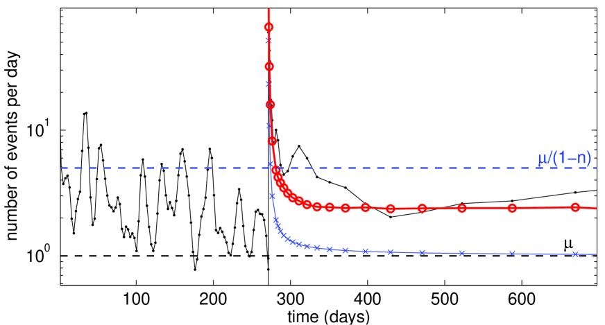
Figure 3: Rate of seismic activity for a synthetic catalog (black dots) generated with the parameters $n=0.8$, $\alpha=0.8$, $b=1$, $c=0.001$ day, $m_{0}=3$ and $\mu=1$ event per day. We compare different methods of prediction of the seismicity rate following a large event $M=7$ that has occurred at the time of the large peak shown in the figure. Using the data up to the present time $t_{i}\leq u$, where $u$ is the “present” taken fixed just after the $M=7$ earthquake, we try to predict the future activity up to 1 year in the future. We use two predictions algorithms: the sum of the bare propagators of all past events $t_{i}\leq u$ (crosses), and the median of the seismicity rate (open circles) obtained over 500 scenarios generated with the ETAS model, using the same parameters as for the synthetic catalog we want to predict, and taking into account the specific realization of the synthetic catalog up to the present.

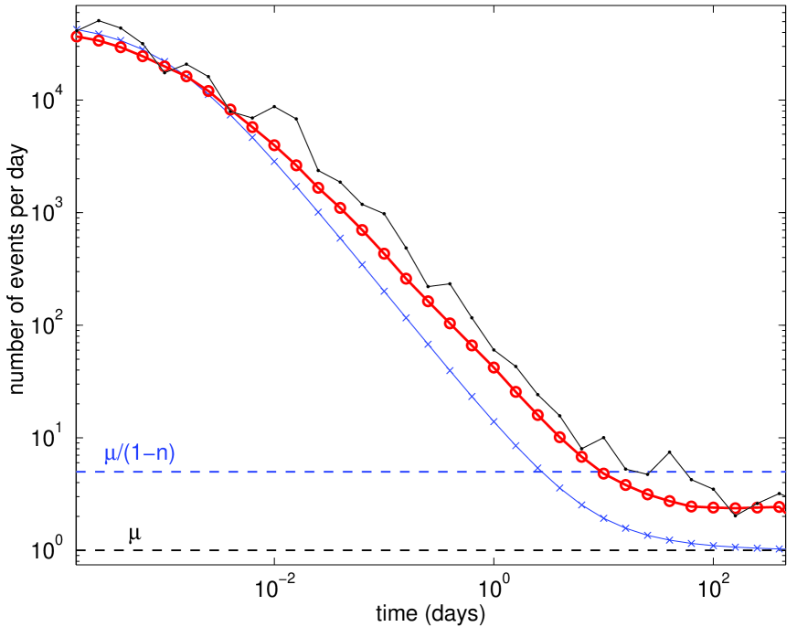
Figure 4: Same as Figure 3 but as a function of the logarithm of the time after the mainshock. At early time $t-u<10^{-2}$ days, the predicted seismicity rate is correctly predicted by the naive bare Omori law shown by the crosses which is indistinguishable from the more elaborate scheme involving all cascades of triggered events. At larger times, the cascade of triggered seismicity renormalizes the seismicity rate to a significantly higher level, which is correctly forecasted by the mean over the 500 scenarios.

Figure 3 illustrates the problem of forecasting the aftershock seismicity following a large $M=7$ event. Imagine that we have just witnessed the $M=7$ event and want to forecast the seismic activity afterward over a varying horizon from days to years in the future. In this simulation, $u$ is kept fixed at the time just after the $M=7$ event and $t$ is varied. A realization of the instantaneous rate of seismic activity (number of events per day) of a synthetic catalog is shown by the black dots. This simulation has been performed with the parameters $n=0.8$, $\alpha=0.8$, $b=1$, $c=0.001$ day, $m_{0}=3$ and $\mu=1$ event per day. This single realization is compared with two forecasting algorithms: the sum of the bare propagators of all past events $t_{i}\leq u$ (crosses), and the median of the seismicity rate obtained over 500 scenarios generated with the ETAS model, using the same parameters as used for generating the synthetic catalog we want to forecast, and taking into account the specific realization of events in each scenario up to the present. Figure 4 is the same as Figure 3 but shows the seismic activity as a function of the logarithm of the time after the mainshock. These two figures illustrate clearly the importance of taking into account all the cascades of still unobserved triggered events in order to forecast correctly the future rate of seismicity beyond a few minutes. The aftershock activity forecast gives a very reasonable estimation of the future activity rate, while the extrapolation of the bare Omori law of the strong $M=7$ event together with the past seismicity very badly under-estimates the future seismicity beyond half-an-hour after the strong event.

5.2 Varying “present” with fixed forecast horizon

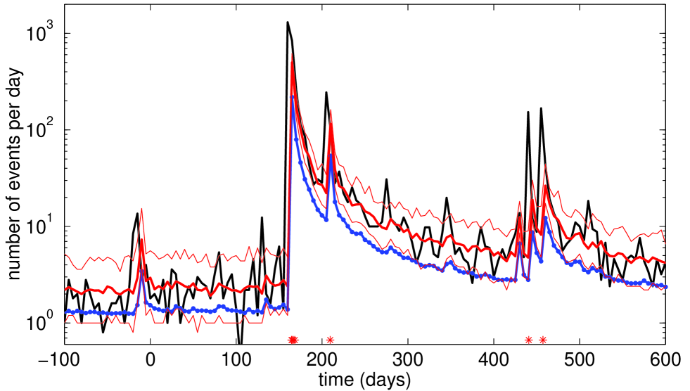
Figure 5: Comparison between the seismicity rate (black line) observed for 5 day time periods, with the predicted seismicity rate using either the sum of the bare propagators of the past seismicity (dots) or using the median of 100 scenarios (gray line) generated with the same parameters as for the synthetic catalog we want to predict, $n=0.8$, $c=0.001$ day, $\mu=1$ event per day, $m_{0}=3$, $b=1$ and $\alpha=0.8$. The thin solid lines indicate the first and 9^th deciles of the set of 100 scenarios: there is 80% probability that the predicted seismicity over the next 5 days falls within these two lines. Stars indicate the occurrence of a large $M\geq 7$ earthquake. Forecasts are updated every 5 days.

Figure 5 compares a single realization of the seismicity rate (open circles) observed and summed over a 5 days period and divided by $5$ so that it is expressed as a daily rate, with the predicted seismicity rate using either the sum of the bare propagators of the past seismicity (dots) or using the median of 100 scenarios (crosses) generated with the same parameters as for the synthetic catalog we want to forecast: $n=0.8$, $c=0.001$ day, $\mu=1$ event per day, $m_{0}=3$, $b=1$ and $\alpha=0.8$. The forecasting methods calculate the total number of events over each 5 day period lying ahead of the present, taking into account all past seismicity including the still unobserved triggered seismicity. This total number of forecasted events is again divided by $5$ to express the prediction as daily rates. The thin solid lines indicate the first and 9^th deciles of the distributions of the number of events observed in the pool of 100 scenarios. Stars indicate the occurrence of large $M\geq 7$ earthquakes. Only a small part of the whole time period used for the forecast is shown, including the largest $M=8.5$ earthquake of the catalog, in order to illustrate the difference between the realized seismicity rate and the different methods of forecasting.

The realized seismicity rate is always larger than the seismicity rate predicted using the sum of the bare propagators of the past activity. This is because the seismicity that will occur up to 5 days in the future is dominated by the seismicity that will be triggered in the near future that is still unobserved but must be taken into account. The realized seismicity rate is close to the median of the scenarios (crosses), and the fluctuations of the realized seismicity rate are in good agreement with the expected fluctuations measured by the deciles of the distributions of the seismicity rate over all scenarios generated.

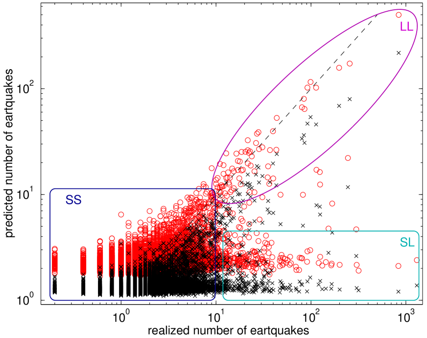
Figure 6: Comparison between the seismicity rate observed for 5 day time periods from the present with the predicted seismicity rate over the same 5 day periods using either the sum of the bare propagators of the past seismicity (crosses) or using the median of 100 scenarios (circles), corresponding to the same data shown in Figure 5 but using a long synthetic catalog of $N=200000$ events over a time period of 150 yrs. The dashed line corresponds to the perfect forecast when the predicted seismicity rate is equal to the realized seismicity rate. This figure shows that the best forecasts are obtained using the median of the scenarios rather than using the bare propagator, which always underestimates the realized seismicity rate. The meaning of the clusters LL, SL and SS are discussed in the text. Forecasts are updated every 5 days. A faster rate of updating does not change the fraction of predictable events lying close to the diagonal.

Figure 6 compares the predictions of the seismicity rate over a 5 day horizon with the seismicity of a typical synthetic catalog; a small fraction of the history was shown in Figure 5. This comparison is performed by plotting the predicted number of events in each 5 day horizon window as a function of the actual number of events. The open circles (crosses) correspond to the forecasts using the median of 100 scenarios (the sum of the bare Omori propagators of the past seismicity). This Figure uses a synthetic catalog of $N=200000$ events of magnitude larger than $m_{0}=3$ covering a time period of 150 yrs. The dashed line corresponds to the perfect prediction when the predicted seismicity rate is equal to the realized seismicity rate. This Figure shows that the best predictions are obtained using the median of the scenarios rather than using the bare propagator, which always underestimates the realized seismicity rate, as we have already shown.

The most striking feature of Figure 6 is the existence of several clusters, reflecting two mechanisms underlying the realized seismicity.

1. cluster LL with large predicted seismicity and large realized seismicity;

2. cluster SL with small predicted seismicity and large realized seismicity;

3. cluster SS with small predicted seismicity and small realized seismicity;

Cluster LL along the diagonal reflects the predictive skill of the triggered seismicity algorithm: this is when future seismicity is triggered by past seismicity. Cluster SL lies horizontally at low predicted seismicity rates and shows that large seismicity rates can also be triggered by an unforecasted strong earthquake, which may occur even when the seismicity rate is low. This expresses a fundamental limit of predictability since the ETAS model permits large events even for low prior seismicity, as the earthquake magnitudes are drawn from the GR independently of the seismic rate. About 20% of the large values of the realized seismicity rate above 10 events per day fall in the LL cluster, corresponding to a predictability of about 20% of the large peaks of realized seismic activity. The cluster SS is consistent with a predictive skill but small seismicity is not usually an interesting target. Note there is no cluster of large predicted seismicity associated with small realized seismicity.

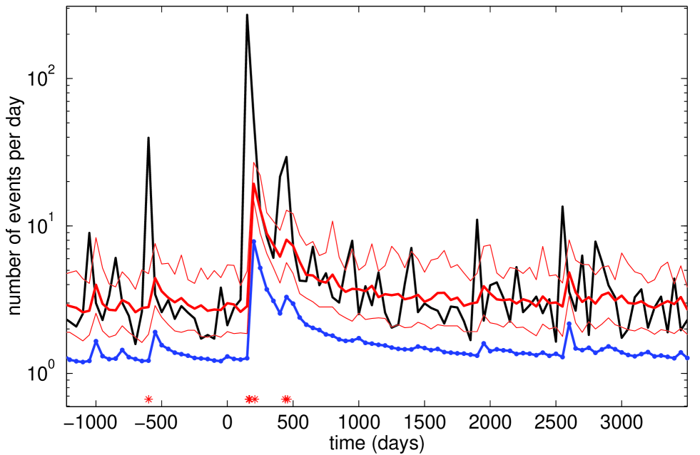
Figure 7: Same as Figure 5 but for a larger horizon $t=50$ days.

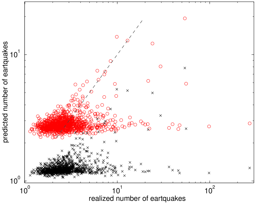
Figure 8: Same as Figure 6 but for a larger horizon $t=50$ days. For such large horizons, taking into account the cascade of triggered seismicity makes a large difference on the performance of the predicted seismicity rate.

Figure 7 is the same as Figure 5 for a longer time window of 50 days, which stresses the importance of taking into account the yet unobserved future seismicity in order to accurately forecast the level of future seismicity. Figure 8 is the same as Figure 6 for the forecast time window of 50 days with forecasts updated each 50 days. Increasing the time window $T$ of the forecasts from 5 to 50 days leads to a smaller variability of the predicted seismicity rate. However, fluctuations of the seismicity rate of one order of magnitude can still be predicted with this model. The ETAS model therefore performs much better than a Poisson process for large horizons of 50 days.

5.3 Error diagrams and prediction gains

In order to quantify the predictive skills of different prediction algorithms for the seismicity of the next five days, we use the error diagram [Molchan, 1991; 1997; Molchan and Kagan, 1992]. The predictions are made from the present to 5 days in the future and are updated each 0.5 day. Using a shorter time between each prediction, or updating the prediction after each major earthquake, will obviously improve the predictions, because large aftershocks occur often just after the mainshock. But in practice the forecasting procedure is limited by the time needed to estimate the location and magnitude of an earthquake. Moreover, predictions made for very short times in advance (a few minutes) are not very useful.

An error diagram requires the definition of a target, for instance $M\geq 6$ earthquakes, and plots the fraction of targets that were not predicted as a function of the fraction of time occupied by the alarms (total duration of the alarms normalized by the duration of the catalog). We define an alarm when the predicted seismic rate is above a threshold. Recall that in our model the seismic rate is the physical quantity that embodies completely all the available information on past events. All targets one might be interested in derive from the seismic rate.

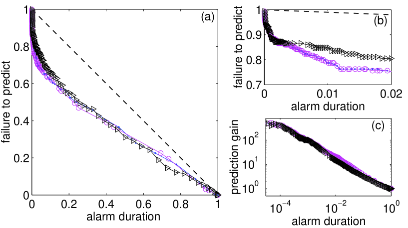
Figure 9: Error diagram of different prediction algorithms, using either the bare propagator (dots), the median (circles) or the mean (triangles) number of events obtained for the scenarios. The synthetic catalog and the prediction methods are the same as for Figures 5 and 6. We use a time horizon (window size) of $T=5$ days to estimate the seismicity rate but we update the predictions each 0.5 day. Target events are $M\geq 6$ earthquakes. An alarm is defined when the predicted seismicity rate is above a threshold. Each point of the curve corresponds to a different threshold ranging from 0.1 to 1000 events per day. The quality of the predictions is measured by plotting the ratio of failures to predict as a function of the total durations of the alarms normalized by the duration of the catalog. The results for these three algorithms are considerably better than those obtained for a random prediction, shown as a dashed line for reference. This Figure shows that about 20% of large peaks of seismic activity can be predicted with a very small alarm duration of about 1%. Panel (b) is a magnification of panel (a) close to the origin of the alarm duration showing the very fast increase of the success fraction ($=1-$ failure to predict) as the alarm duration increases from $0$. Panel (c) shows that the predicted gain, defined as the ratio of the success fraction over the alarm duration, decays as a function of the alarm duration from a very high value obtained for very short alarm durations as an approximate inverse power law with exponent slightly larger than $1/2$.

Figure 9 presents the error diagram for $M\geq 6$ targets, using a time window $T=5$ days to estimate the seismicity rate, and a time $dT=0.5$ days between two updates of the predictions. We use different prediction algorithms, either the bare propagator (dots), the median (circles) or the mean (triangles) number of events obtained for the 100 scenarios already generated to obtain Figures 5 and 6. Each point of each curve corresponds to a different threshold ranging from 0.1 to 1000 events per day. The results for these three prediction algorithms are considerably better than those obtained for a random prediction, shown as a dashed line for reference.

Ideally, one would like the minimum numbers of failures and the smallest possible alarm duration. Hence, a perfect prediction corresponds to points close to the origin. In practice, the fraction of failure to predict is 100% without alarms and the gain of the prediction algorithm is quantified by how fast the fraction of failure to predict decreases from 100% as the fraction of alarm duration increases. Formally, the gain $G$ reported below is defined as the ratio of the fraction of predicted targets ($=1-$ number of failures to predict) divided by the fraction of time occupied by alarms. A completely random prediction corresponds to $G=1$.

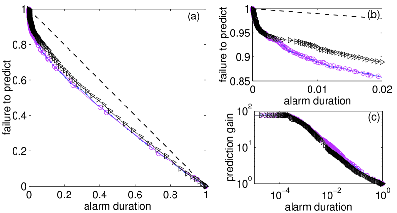
Figure 10: Same as Figure 9 but for targets with lower magnitudes $M\geq 5$. Panel (c) shows that the predicted gain is again approximately an inverse power law with exponent close to $1/2$ as a function of the alarm duration.

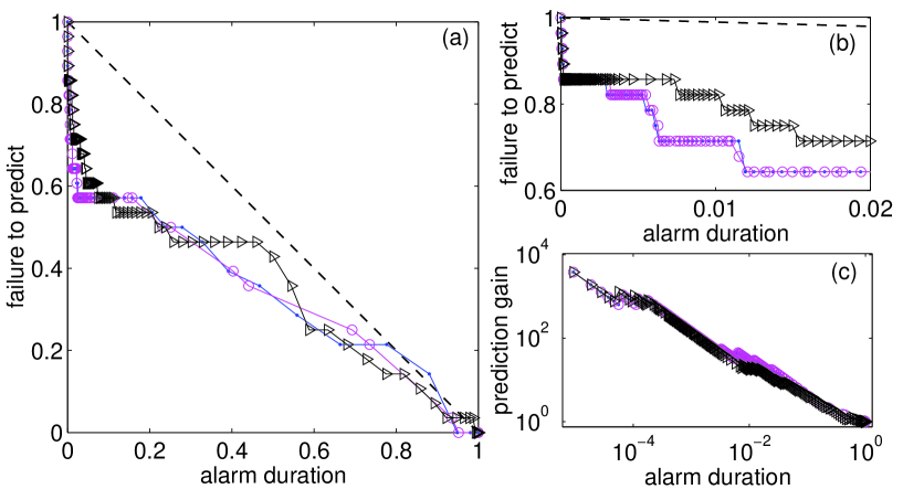
Figure 11: Same as Figure 9 but for targets with larger magnitudes $M\geq 7$. Panel (c) shows that the predicted gain is again approximately an inverse power law with exponent slightly smaller than $1$ as a function of the alarm duration. Comparing this figure with Figures 9 and 10 suggests that the exponent defined in panel (c) is slowly increasing with the magnitude of the targets.

We observe that about $50\%$ of the $M\geq 6$ earthquakes can be predicted with a small fraction of alarm duration of about $20\%$, leading to a gain of $2.5$ for this value of the alarm duration. The gain is significantly stronger for shorter fractions of alarm duration: as shown in panel (b) of Figure 9, 25% of the $M\geq 6$ earthquakes can be predicted with a small fraction of alarm duration of about $2\%$, leading to a gain of $12.5$. The origin of this good performance for only a fraction of the targets has been discussed in relation with Figure 6, and is associated with those events that occur in times of large seismic rate (cluster along the diagonal in Figure 6). Panel (c) of Figure 9 shows the dependence of the prediction gain $G$ as a function of the alarm duration: the three prediction schemes give approximately the same power law increase with an exponent close to $1/2$ of the gain as the duration of alarm decreases. For small alarm duration, the gain reaches values of several hundreds. The saturation at very small values of the alarm duration is due to the effect that only a few targets are sampled. Figures 10 and 11 are similar to Figure 9, respectively for a smaller target of magnitudes larger than $5$ and a larger target of magnitudes larger than $7$.

Table 6 presents the results for the prediction gain and for the number of successes using different choices of the time window $T$ and of the update time $dT$ between two predictions, and for different values of the target magnitude between 5 and 7. The prediction gain decreases if the time between two updates of the prediction increases, because most large earthquakes occur at very short times after a previous large earthquake. In contrast, the prediction gains do not depend on the time window $T$ for the same value of the update time $dT$.

The prediction gain is observed to increase significantly with the target magnitude, especially in the range of small fraction of alarm durations (see Table 6 and Figures 9-11). However, this increase of the prediction gain does not mean that large earthquakes are more predictable than smaller ones, in contrast with, for example, the critical earthquake theory [Sornette and Sammis, 1995; Jaumé and Sykes, 1999; Sammis and Sornette, 2002]. In the ETAS model, the increase of the prediction gain with the target magnitude is due to the decrease of the number of target events with the target magnitude. Indeed, choosing $N$ events at random in the catalog independently of their magnitude gives on average the same prediction gain as for the $N$ largest events. This demonstrates that the larger predictability of large earthquakes is solely a size effect.

We now clarify the statistical origin of this size effect. Let us consider a catalog of total duration $D$ with a total number $N$ of events analyzed with $D/T$ time windows with horizon $T$. These $D/T$ windows can be sorted by decreasing seismicity $r_{1}>r_{2}>...>r_{n}>...$, where $r_{i}$ is the $i$-th largest number of events in a window of size $T$. There are $n_{1},n_{2},...,n_{i},...$ windows of type $1,2,...,i,...$ respectively, such that $\sum_{i}r_{i}~{}n_{i}=N$. Then, the frequency-probability that an earthquake drawn at random from the catalog falls within a window of type $i$ is

$$p_{i}={r_{i}~{}n_{i}\over N}~{}.$$ (28)

We have found that, over more than three decades spanning from $1$ event to $10^{3}-10^{4}$ events per window, the cumulative distribution of these $p_{i}$’s is a power law with exponent approximately equal to $\kappa=0.4$. This power law is found for the observable realized seismicity as well as for the seismicity predicted by the different methods discussed above. Such a small exponent $\kappa$ implies that the few windows that happen to have the largest number of events contain a significant fraction of the total seismicity. It can be shown [Feller, 1971] that, in absence of any constraint, the single window with the largest number of events contains on average $1-\kappa=60\%$ of the total seismicity. This would imply that there is a $60\%$ probability that an earthquake drawn at random within the catalog (of $150$ years) belongs to this single window of $5$ days. This effect is moderated because the random variables $p_{i}$ have to sum up to $1$ by definition. This can be shown to entail a roll-off of the cumulative distribution depleting the largest values of $p_{i}$. Empirically, we find that the most active window out of the approximately $54,000$ daily windows of our $150$ years long catalog contains only $3\%$ of the total number of events. While this value of $3\%$ is smaller than the prediction of 60% in absence of normalization, it is considerably larger than the “democratic” result which would predict a fraction of about $0.002\%$ of the seismicity in each window. Since a high seismicity rate implies strong interactions and triggering between earthquakes and is usually associated with recent past high seismicity; the events in such a window are highly predictable. When the number of targets increases, one starts to sample statistically other windows with smaller seismicity which have a weaker relation with triggered seismicity and thus present less predictive power.

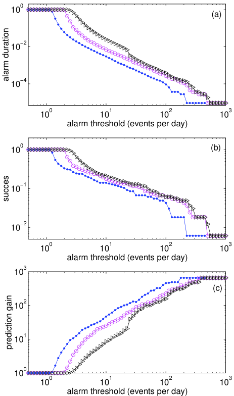
Figure 12: Analysis of the prediction methods, using the same synthetic catalog and predictions methods as for Figures 5-11. We use a time window $T=5$ days to estimate the predicted seismicity rate, and a time $dT=0.5$ days between two updates of the prediction. Target events are $M\geq 6$ earthquakes. The duration of alarms normalized by the total duration of the catalog is shown in panel (a) as a function of the alarm threshold for the three predictions methods : bare propagator (dots), the median (circles) and the mean (triangles) number of events obtained for the scenarios. The proportion of successes is shown in panel (b). The prediction gain shown in panel (c) is defined by the ratio of the proportion of successes (b) over the duration of alarms (a). The prediction gain for large values of the alarm threshold is significantly higher that the random prediction gain equal to $1$.

In our previous discussion, we have not distinguished the skills of the three algorithms, because they perform essentially identically with respect to the assigned targets. This is very surprising from the perspective offered by all our previous analysis showing that the naive use of the direct Omori law without taking into account the effect of any indirect triggered seismicity strongly underestimate the future seismicity. We should thus expect a priori that this prediction scheme should be significantly worse than the two others based on a correct counting of all unobserved triggered seismicity. The explanation for this paradox is given by examining Figure 12, which presents further insight in the prediction methods applied to the synthetic catalogs used in Figures 3-11. Figure 12 shows three quantities as a function of the threshold in seismicity rate used to define an alarm, for each of the three algorithms. These quantities are respectively the duration of alarms normalized by the total duration of the catalog shown in panel (a), the fraction of successes ($=1-$ failure to predict) shown in panel (b) and the prediction gain shown in panel (c). These three panels tell us that the incorrect level of seismic activity predicted by the bare Omori law approach can be compensated by the use of a lower alarm threshold. In other words, even if the seismicity rate predicted by the bare Omori law approach is wrong in absolute values, its time evolution in relative terms contains basically the same information as the full-fledged method taking into account all unobserved triggered seismicity. Therefore, an algorithm that can detect a relative change of seismicity can perform as well as the complete approach for the forecast of the assigned targets. This is an illustration of the fact that predictions of different targets can have very different skills which depend on the targets. Using the full-fledged renormalized approach is the correct and only method to get the best possible predictor of future seismicity rate. However, other simpler and more naive methods can perform almost as well for more restricted targets, such as the prediction of only strong earthquakes.

5.4 Optimization of earthquake prediction

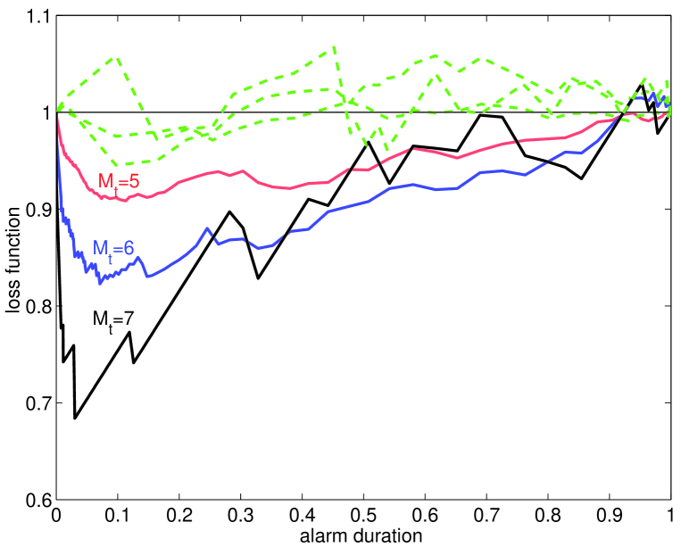
Figure 13: Loss function $\gamma$ defined as the sum of the fraction of missed events and of the fraction of alarms. We use the same catalog and prediction method as in Figures 5-12, with a time window of 5 days, and an update time of 0.5 days. Solid lines give the results for the prediction algorithm based on the ETAS model (average of the seismicity rate over 100 scenarios) for different values of the target magnitudes. Dashed lines correspond to the predictions made using a Poisson process, with a seismicity rate equal to the average seismicity rate of the catalog.

The optimization of the prediction method requires the definition of a loss function $\gamma$, which should be minimized in order to determine the optimum alarm threshold of the prediction method. The probability gain defined in the previous section cannot be used as an optimization method, because it is maximum for zero alarm time. The strategies that optimize the probability gain are thus very impractical. An error function commonly used [e.g., Molchan and Kagan, 1992] is the sum of the two types of errors in earthquake prediction, the fraction of alarm duration $\tau$ and the fraction of missed events $\nu$. This loss function is illustrated in Figure 13 for the same numerical simulation of the ETAS model as in the previous section, using a prediction time window of 5 days and an update time of 0.5 day, for different values of the target magnitude between 5 and 7. For a prediction algorithm that has no predictive skill, the loss function $\gamma$ should be close to 1, independently of the alarm duration $\tau$. This is indeed what we observe for the prediction algorithm using a Poisson process, with a constant seismicity rate equal to the average seismicity rate of the realized simulation. For the prediction methods based on the ETAS model, we obtain a significant predictability by comparison with the Poisson process (Figure 13). The loss function is minimum for a fraction of alarm duration of about 10%, and decreases with the target magnitude $M_{t}$ from 0.9 for $M_{t}=5$ down to 0.7 for $M_{t}=7$. We expect that the minimum loss function will be much lower when using the information on earthquake locations.

5.5 Influence of the ETAS parameters on the predictability

We now test the influence of the model parameters $\alpha$, $n$, $m_{0}$ and $p$ on the predictability. We did not test the influence of the $b$-value, because this parameter is rather well constrained in seismicity, and because its influence is felt only relative to $\alpha$. We keep $c$ equal to 0.001 day because this parameter is not critical as long as it is small. The external loading $\mu$ is also fixed to 1 event/day because it is only a multiplicative factor of the global seismicity. The value of the minimum magnitude $m_{0}$ above which earthquakes may trigger aftershocks of magnitude larger than $m_{0}$ is very poorly constrained. This value is no larger than $3$ for the Southern California seismicity, because there are direct evidences of $M3+$ earthquakes triggered by $M=3$ earthquakes [Helmstetter, 2003]. We are limited in our exploration of small values of $m_{0}$ because the number of earthquakes increases rapidly if $m_{0}$ decreases, and thus the computation time becomes prohibitive. We have tested the values $m_{0}=1$ and $m_{0}=2$ and find that the effect of a decrease of $m_{0}$ is simply to multiply the seismicity rate obtained for $M\geq 3$ by a constant factor. Using a smaller $m_{0}$ does not change the temporal distribution of seismicity and therefore does not change the predictability of the system.

We use the minimum value of the error function $\gamma$ introduced in the previous section to characterize the predictability of the system. This function is estimated from the seismicity rate predicted using the bare propagator, as done in previous studies [Kagan and Knopoff, 1987; Kagan and Jackson, 2000]. While all three prediction methods that we have investigated give approximately the same results for the error diagram, the method of the bare propagator is much faster, which justifies to use it. The results are summarized in Table 6, which gives the minimum value of the error function $\gamma$ for each set of parameters, and the corresponding values of the alarm duration, the proportion of predicted $M\geq 6$ events and the prediction gain. All values of $\gamma$ are in the range 0.6-0.9, corresponding to a small but significant predictability of the ETAS model. The predictability increases (i.e, $\gamma$ decreases) with $\alpha$, $n$ and $p$, because for large $\alpha$, large $n$ and/or large $p$, there are larger fluctuations of the seismicity rate which have stronger impacts for the future seismicity. The minimum magnitude $m_{0}$ has no significant influence on the predictability. We recover the same pattern when using another estimate of the predictability measured by the prediction gain $G_{1\%}$ for an alarm duration of $1\%$.

5.6 Information gain

We now follow Kagan and Knopoff [1977], who introduced the entropy/information concept linking the likelihood gain to the entropy per event and hence to the predictive power of the fitted model, and Vere-Jones [1998], who suggested using the information gain to compare different models and to estimate the predictability of a process.

Our forecasting algorithm provides the average seismicity rate $\lambda_{i}$ above $m_{0}$ in the time interval $(t_{i},t_{i}+T)$. Assuming a constant magnitude distribution given by (5), the probability $p_{i}$ to have at least one event above the target magnitude $M_{t}$ in the time interval $(t_{i},t_{i}+T)$ can be evaluated from the average seismicity rate $\lambda_{i}$ by

$$p_{i}=1-\exp\Bigl{(}-\lambda_{i}~{}10^{-b(M_{t}-m_{0})}\Bigr{)}~{}.$$ (29)

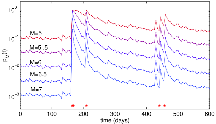
Figure 14: Probability $p_{M}(t)$ of having at least an event of magnitude larger than $M$ in the time interval $(t,t+T)$ with T=5 days. We have evaluated $p_{M}$ for $M$ between 5 and 7, from the seismicity rate predicted by the median of 100 scenarios, and using equation (29) to estimate the probability $p_{M}(t)$ from the average seismicity rate $\lambda(t)$ in the time interval $(t,t+T)$. $p_{M}(t)$ is plotted for the sequence shown in Figure 5. Stars indicate the occurrence of a large $M\geq 7$ earthquake. The largest $M=8.55$ event of the sequence occurs at time $t=164$ days when the seismicity rate is close to the average value. Thus, this event cannot be predicted. Six large $M>7$ earthquakes occur in the following 500 days when the seismicity rate is still above its average value, including three $M>7$ events in the 5 days immediately following the great event.

Figure 14 shows the probability $p_{i}$ obtained for different choices of the target magnitude $M_{t}$ for the same sequence as in Figure 5.

The binomial score $B$ compares the prediction $p_{i}$ with the realization $X_{i}$, with $X_{i}=1$ if a target event occurred in the interval $(t_{i},t_{i}+T)$ and $X_{i}=0$ otherwise. For the whole sequence of intervals $(t_{i},t_{i}+T)$, the binomial score is defined by

$$B=\sum_{i}\Bigl{[}X_{i}\log(p_{i})+(1-X_{i})\log(1-p_{i})\Bigr{]}~{},$$ (30)

where the sum is performed over all (non-overlapping) time windows covering the whole duration of the catalog. The first term represents the contribution to the score from those intervals which contain an event, and the second term the contribution to the score from those intervals which contain no event.

In order to test the performance of a forecasting algorithm, we compare the binomial score $B$ of the forecast with the binomial score of a Poisson process. We use two definitions of the Poisson process. First, we use the same definition as in [Vere-Jones, 1998] and take a Poisson process with a seismicity rate equal to the average seismicity rate of the realized catalog and use equation (29) to estimate the probability of having at least an event above the target magnitude in each time interval. Because this definition of the probability assumes a uniform temporal distribution of target events and thus neglects clustering of large events, it over-estimates the proportion of intervals which have at least one target event. Indeed, the probability of having several events of magnitude $M\geq M_{t}$ in the same time window is much higher for the ETAS model than for a Poisson process. We thus propose another definition of the Poisson process defined by putting all values of $p_{i}$ equal to the fraction of intervals in the realized catalog that have at least a target events. For small time intervals and/or large target magnitudes, the proportion of intervals that have several target events is very small, and the two definitions of the Poisson process give similar results. The results for different choices of the time interval $T$ and of the target magnitude $M_{t}$ are listed in Table 6.

We evaluate the binomial score $B$ for different prediction algorithms: (i) the average of the seismicity rate over all scenarios ($B_{mean}$), (ii) the exponential of the average of the logarithm of the mean of the seismicity rate ($B_{meanl}$), (iii) the median of the seismicity rate ($B_{med}$) and (iv) the sum of the bare propagators of the past seismicity ($B_{\phi}$). The results for the forecasting methods based on the median seismicity rate ($B_{med}$ and $B_{meanl}$) are in general better than the Poisson process, i.e., the binomial score for the forecasting algorithms are larger than the score obtained with a Poisson process for both definitions of the Poisson process. The binomial score $B_{pois2}$ measured using the second definition of the Poisson process is higher than the binomial score $B_{pois1}$ for the first definition of the Poisson process because the first method is biased and over-estimates the probability of having at least a target event. The scores of the forecasting methods which take into account the cascade of secondary aftershocks ($B_{med}$, $B_{mean}$ and $B_{meanl}$ in Table 6) are significantly better than the score $B_{\phi}$ obtained with the bare propagator, even for short time intervals $T$, because this predictor under-estimates the realized seismicity rate. Similarly, the score $B_{mean}$ obtained for the average seismicity rate is generally smaller than $B_{med}$ because the averaging method generally over-estimates the realized seismicity rate. For large time intervals $T\geq 10$ days, and for large target magnitudes, the results for the bare propagator are even worse than the results obtained with a Poisson process using both definitions of the Poisson process.

Our results are in disagreement with those reported in Vere-Jones [1998] on the same ETAS model: we conclude that the ETAS model has a significantly higher predictive power than the Poisson process while Vere-Jones [1998] concludes that the forecasting performance of the ETAS model is worse than with the Poisson model. Vere-Jones and Zhuang’s procedure and ours are very similar. They use the same method to generate ETAS simulations and to update the predictions at rigid time intervals, with a similar time between two updates of the predictions. They use the same method to estimate the probability of having a target event for the Poisson process (corresponding to our first definition of the Poisson process) but a different method to estimate the probability $p_{i}$ for the ETAS model. Rather than using eq. (29) to derive the probability $p_{i}$ from the seismicity rate as done in this work, they measure directly this probability from the fraction of scenarios which have at least a target event. We have compared the two methods and found that the method of Vere-Jones is very similar to the results derived from the median seismicity rate. However, for large target events and small time intervals, the method of Vere-Jones requires to generate a huge number of scenarios to obtain accurate estimates of the fraction of scenarios which have at least a target event. We thus believe that our method might be better in this case and give a more accurate estimate of the probability $p_{i}$ of having at least a target event. This is one possible origin of the discrepancy between Vere-Jones’ results and ours.

The ETAS parameters used in the two studies are also very similar and cannot account for the disagreement. The tests of Vere-Jones [1998] have been performed using a $\alpha/b$ ratio of $0.57/1.14=0.5$ smaller than the value $\alpha/b=0.8$ used in our simulations. This difference may lead to a smaller predictability for the simulations of Vere-Jones [1998] because there are fewer large aftershock sequences. The branching ratio $n=0.78$ used by Vere-Jones [1998] is very close to our value $n=0.8$. However, these difference in the ETAS parameters cannot explain why Vere-Jones [1998] obtains a better predictability for a Poisson process than for the ETAS model. Vere-Jones [1998] concludes that the Poisson process is better predictive than ETAS because the binomial score measured for time periods containing target events, i.e., by taking only the first term of eq. (30), is larger for the Poisson process than for ETAS. While we agree with this point, we note that the fact that the first term of the binomial score is larger for the Poisson process than for ETAS does not imply that the Poisson process is more predictive. Indeed, the score for periods containing events is maximum for a simple model specifying a probability $p_{i}=1$ of having an event for all time intervals. Because this simple model does not miss any event, it gives the maximum binomial score for periods containing target events, but is of course not better than the ETAS or the Poisson model if we take into account the second term of the binomial score corresponding to periods without target events. If we take our second definition of the Poisson process, taking into account clustering, we obtain a better score with the ETAS model for periods containing target events than for the Poisson process. We thus think that the conclusion of Vere-Jone [1998] that the ETAS model is sometimes less predictive than the Poisson process is due to an inadequate measure of the predictability. We thus caution that a suitable assessment of the forecasting skills of a model requires several complementary quantitative measures, such as the predicted versus realized seismicity rates, the error diagram and predictability gain and the entropy-information gains, and a large number of target events.

6 Conclusions

Using a simple model of triggered seismicity, the ETAS model, based on the (bare) Omori law, the Gutenberg-Richter law and the idea that large events trigger more numerous aftershocks, we have developed an analytical approach to account for the triggered seismicity adapted to the problem of forecasting future seismic rates at varying horizons from the present. Tests presented on synthetic catalogs have validated the use of interacting triggered seismicity to forecast large earthquakes in these models. This work provides what we believe is a useful benchmark from which to develop real prediction tests of real catalogs. These tests have also delineated the fundamental limits underlying forecasting skills, stemming from an intrinsic stochastic component in the seismicity models. Our results offer a rationale for the fact that pattern recognition algorithms may perform better for strong earthquakes than for weaker events. Although the predictability of an earthquake is independent of its magnitude in the ETAS model, the prediction gain is better for the largest events because they are less numerous and it is thus more probable that they are associated with periods of large seismicity rates, which are themselves more predictable.

We have shown in Helmstetter et al. [2003] that most precursory patterns used in prediction algorithms, such as a decrease of $b$-value or an increase of seismic activity can be reproduced by the ETAS model. If the physics of triggering is fully characterized by the class of models discussed here, this suggests that patterns and precursory indicators are sub-optimal compared with the prediction based on a full modeling of the seismicity. The calibration of the ETAS model or some of its variants on real catalogs as done in Kagan and Knopoff [1987], Kagan and Jackson [2000], Console and Murru [2001], Ogata [1988, 1989, 1992, 1999, 2001], Kagan [1991], Felzer et al. [2002] represent important steps in this direction. However, in practical terms, the issue of the model errors associated with the use of an incorrect model calibrated on an incomplete data set with not fully known parameters may make this statement weaker or even turn it on its head.

We are very grateful to D. Harte, Y.Y. Kagan, Y. Ogata, F. Schoenberg, D. Vere-Jones and J. Zhuang for useful exchanges and for their feedback on the manuscript. This work is partially supported by by NSF-EAR02-30429, by the Southern California Earthquake Center (SCEC) and by the James S. Mc Donnell Foundation 21st century scientist award/studying complex system.

Console, R. and M. Murru, A simple and testable model for earthquake clustering, J. Geophys. Res., 166, 8699-8711, 2001.

Feller, W., An Introduction to Probability Theory and its Applications, vol. II (John Wiley and sons, New York, 1971).

Felzer, K. R., T. W. Becker, R. E. Abercrombie, G. Ekström and J. R. Rice, Triggering of the 1999 $M_{W}$ $7.1$ Hector Mine earthquake by aftershocks of the 1992 $M_{W}$ $7.3$ Landers earthquake, J. Geophys. Res., 107, doi:10.1029/2001JB000911, 2002.

Gabrielov, A., I. Zaliapin, W. I. Newman and V. I. Keilis-Borok, Colliding cascades model for earthquake prediction, Geophys. J. Int., 143, 427-437, 2000.

Guo, Z. and Y. Ogata, Correlations between characteristic parameters of aftershock distributions in time, space and magnitude, Geophys. Res. Lett., 22, 993-996, 1995.

Guo, Z. and Y. Ogata, Statistical relations between the parameters of aftershocks in time, space and magnitude, J. Geophys. Res., 102, 2857-2873, 1997.

Gutenberg, B. and C. F. Richter, Frequency of earthquakes in California, Bull. Seism. Soc. Am., 34, 185-188, 1944.

Hawkes, A. G., Point spectra of some mutually exciting point processes. J. Roy. Stat. Soc. B , 33, 438-443, 1971.

Hawkes, A. G, Spectra of some mutually exciting point processes with associated variables, In Stochastic Point Processes, ed. P.A.W. Lewis, Wiley, 261-271, 1972.

Helmstetter, A., Is earthquake triggering driven by small earthquakes?, submitted to Phys. Rev. Lett., 2003.

Helmstetter, A. and D. Sornette, Sub-critical and super-critical regimes in epidemic models of earthquake aftershocks, J. Geophys. Res., 107, 2237, 10.1029/2001JB001580, 2002a.

Helmstetter, A. and D. Sornette, Diffusion of epicenters of earthquake aftershocks and Omori’s law: exact mapping to generalized continuous-time random walk model, Physical Review E, 66, 061104, 2002b.

Helmstetter, A. and D. Sornette, Importance of direct and indirect triggered seismicity in the ETAS model of seismicity, in press in Geophys. Res. Lett., 2003.

Helmstetter, A, D. Sornette and J.-R. Grasso, Mainshocks are aftershocks of conditional foreshocks: How do foreshock statistical properties emerge from aftershock laws, J. Geophys. Res., 108, 2046,
doi:10.1029/2002JB001991, 2003.

Jaumé, S. C. and L. R. Sykes, Evolving towards a critical point: A review of accelerating seismic moment/energy release prior to large and great earthquakes, Pure Appl. Geophys., 155, 279-305, 1999.

Kagan, Y. Y., Statistical methods in the study of the seismic process (with discussion: comments by M. S. Bartlett, A. G. Hawkes, and J. W. Tukey), Bull. Int. Statist. Inst., 45 (3), 437-453, 1973.

Kagan, Y. Y., Likelihood analysis of earthquake catalogues Geophys. J. Int., 106, 135-148, 1991.

Kagan, Y. Y., Universality of the seismic moment-frequency relation, Pure Appl. Geophys., 155, 537-573, 1999.

Kagan, Y., and L. Knopoff, Earthquake risk prediction as a stochastic process, Phys. Earth Planet. Inter., 14, 97-108, 1977.

Kagan Y.Y. and L. Knopoff, Spatial distribution of earthquakes: the two-point correlation function, Geophys. J. R. Astr. Soc., 62, 303-320, 1980.

Kagan, Y. Y. and L. Knopoff, Statistical short-term earthquake prediction, Science, 236, 1563-1467, 1987.

Kagan, Y. Y. and D. D. Jackson, Probabilistic forecasting of earthquakes, Geophys. J. Int., 143, 438-453, 2000.

Keilis-Borok V. I. and L. N. Malinovskaya, One regularity in the occurrence of strong earthquakes, J. Geophys. Res., 69, 3019-3024, 1964.

Keilis-Borok V. I. and V. G. Kossobokov, Premonitory activation of seismic flow: algorithm $M8$, Phys. Earth Planet. Inter., 61, 73-83, 1990a.

Keilis-Borok V. I. and V. G. Kossobokov, Times of increased probability of strong earthquakes ($M\geq 7.5$) diagnosed by algorithm $M8$ in Japan and adjacent territories, J. Geophys. Res., 85, 12413-12422, 1990b.

Keilis-Borok V. I. and A. Soloviev, Nonlinear Dynamics of the Lithosphere and Earthquake Prediction, 337p, Springer-Verlag Berlin, 2003.

Kisslinger, C., The stretched exponential function as an alternative model for aftershock decay rate, J. Geophys. Res., 98, 1913-1921, 1993.

Kossobokov, V. G., J. H. Healy and J. W. Dewey, Testing an earthquake prediction algorithm, Pure Appl. Geophys., 149, 219-232, 1997.

Kossobokov, V. G., L. L. Romashkova, V. I., Keilis-Borok and J. H. Healy, Testing earthquake prediction algorithms: statistically significant advance prediction of the largest earthquakes in the Circum-Pacific, 1992-1997, Phys. Earth Planet. Inter., 111, 187-196, 1999.

Lomnitz, C., Global Tectonics and Earthquake Risk (Chapter 7 Modelling the earthquake process), Elsevier, 1974.

Molchan, G. M., Structure of optimal strategies in earthquake prediction, Tectonophysics, 193, 267-276, 1991.

Molchan, G. M., and Y. Y. Kagan, Earthquake prediction and its optimization, J. Geophys. Res, 97, 4823-4838, 1992.

Molchan, G. M., Earthquake prediction as a decision-making problem, Pure Appl. Geophys., 149, 233-247, 1997.

Morse, P. M. and H. Feshbach, Methods in Theoretical Physics, McGraw-Hill, New-York, 1953.

Ogata, Y., Statistical models for earthquake occurrences and residual analysis for point processes, Research Memo. (Technical report), No. 288, The Institute of Statistical Mathematics, Tokyo, 1985.

Ogata, Y., Long-term dependence of earthquake occurrences and statistical models for standard seismic activity, Suri Zisin Gaku (Mathematical Seismology) II (ed. Saito, M.), Cooperative Research Report, vol. 3, Institute of Statistical Mathematics, Tokyo, pp. 115-125, 1987 (in Japanese).

Ogata, Y., Statistical models for earthquake occurrence and residual analysis for point processes, J. Am. Stat. Assoc., 83, 9-27, 1988.

Ogata, Y., Statistical model for standard seismicity and detection of anomalies by residual analysis, Tectonophysics, 169, 159-174, 1989.

Ogata, Y., Detection of precursory relative quiescence before great earthquakes though a statistical model, J. Geophys. Res., 97, 19845-19871, 1992.

Ogata, Y., Seismicity analysis through point-process modeling: a review, Pure Appl. Geophys., 155, 471-507, 1999.

Ogata, Y., Increased probability of large earthquakes near aftershock regions with relative quiescence, J. Geophys. Res., 106, 8729-8744, 2001.

Omori, F., On the aftershocks of earthquakes, J. Coll. Sci. Imp. Univ. Tokyo, 7, 111-120, 1894.

Pepke, S. L. and J. L. Carlson, Predictability of self-organizing systems, Phys. Rev. E, 50, 236-242, 1994.

Pepke, S. L., J. L. Carlson and B. E. Shaw, Prediction of large events on a dynamical model of a fault, J. Geophys. Res., 99, 6769-6788, 1994.

Reasenberg, P. A. and L. M. Jones, earthquake hazard after a mainshock in California, Science, 243, 1173-1176, 1989.

Rundle, P. B., J. B. Rundle, K. F. Tiampo, J. S. S. Martins, S. McGinnis and W. Klein, Nonlinear network dynamics on earthquake fault systems, Phys. Rev. Lett., 87, 141-143, 2001.

Rundle, J. B., K. F. Tiampo, W. Klein and J. S. S. Martins, Self-organization in leaky threshold systems: The influence of near-mean field dynamics and its implications for earthquakes, neurobiology, and forecasting, Proc. Nat. Acad. Sci. USA, 99, 2514-2521, 2002.

Sammis, S.G. and D. Sornette, Positive Feedback, Memory and the Predictability of Earthquakes, Proc. Nat. Acad. Sci. USA, 99 SUPP1:2501-2508, 2002.

Sornette, A. and D. Sornette, Renormalization of earthquake aftershocks, Geophys. Res. Lett., 26, 1981-1984, 1999.

Sornette, D. and C. G. Sammis, Complex critical exponents from renormalization group theory of earthquakes : Implications for earthquake predictions, J. Phys. I France, 5, 607-619, 1995.

Sornette D. and A. Helmstetter, On the occurrence of finite-time-singularity in epidemic models of rupture, earthquakes and starquakes, Phys. Rev. Lett., 89, 158501, 2002.

Utsu, T., Aftershocks and Earthquake Statistics (II): Further investigation of aftershocks and other earthquake sequence based on a new classification of earthquake sequences, J. Faculty Sci. Hokkaido Univ. Ser. VII 3, pp. 379-441 , 1970.

Utsu, T., A review of seismicity, Suri Zisin Gaku (Mathematical Seismology) II (ed. Saito, M.), Cooperative Research Report, vol. 34, Institute of Statistical Mathematics, Tokyo, pp. 139-157, 1992 (in Japanese).

Utsu, T., Y. Ogata and S. Matsu’ura, The centenary of the Omori Formula for a decay law of aftershock activity, J. Phys. Earth, 43, 1-33, 1995.

Vere-Jones, D., Probabilities and information gain for earthquake forecasting, Computational seismology, 30, 248-263, 1998.

Wiemer, S, Introducing probabilistic aftershock hazard mapping. Geophys. Res. Lett., 27, 3405-3408, 2000.

ccrrrrrrrrrrrr 40pc 1 Prediction gain for different choices of the alarm duration, and/or different values of the time interval $T$, of the update time $dT$, and of the target magnitude $M_{t}$. $N_{1}$ is the number of targets $M\geq M_{t}$; $N_{2}$ is the number of intervals with at least one target. $G_{max}$ is the maximum prediction gain, which is realized for an alarm duration $A$ (in proportion of the total duration of the catalog), which is also given in the table. All three prediction algorithms used here provide the same gain as a function of the alarm duration, corresponding to different choices of the alarm threshold on the predicted seismicity rate. $N_{s}$ is the number of successful predictions, using the alarm threshold that provides the maximum predictions gain $G_{max}$ for an alarm duration $A$ (we count only one success when two events occur in the same interval). This number $N_{s}$ is always very small, but a much larger number of successes can be obtained with a larger alarm duration. $N_{1\%}$, $N_{10\%}$, $N_{50\%}$ are the number of successes corresponding to an alarm duration (in proportion of the total duration of the catalog) of $1\%$, $10\%$ and $50\%$ respectively, corresponding to the prediction gains $G_{1\%}$, $G_{10\%}$ and $G_{50\%}$. The values of $G_{50\%}$ show a saturation in the predictive power when increasing the fraction of alarm time, reflecting the fundamental limitation stemming from the fraction of large earthquakes not associated with a large seismic rate. Reading for instance of the last line of this table, we observe that, out of 26 time windows of $50$ days that contained a $M\geq 7$ earthquake, we are able to predict 7 of them with only $1\%$ of the time occupied by alarms. Only two additional ones are predicted when using $10\%$ of the time occupied by alarms. And only another four are predicted by increasing the time of alarms to half the total duration of the catalog. The catalog spans 150 years corresponding to a little more than $10^{5}$ half-day periods. T & dT $M_{t}$ $N_{1}$ $N_{2}$ $G_{max}$ $A$ $N_{s}$ $N_{1\%}$ $N_{10\%}$ $N_{50\%}$ $G_{1\%}$ $G_{10\%}$ $G_{50\%}$
(days) (days) 1.0 &1.0 5.0 2003 1332 40.4 $3.2\times 10^{-4}$ 171203328069.012.491.21 1.0 1.0 5.5 637 461 117. $7.4\times 10^{-5}$ 4 5813630312.62.951.311.0 1.0 6.0 198 159 339. $3.7\times 10^{-5}$ 2 30 56 9418.93.521.181.0 1.0 6.5 66 55 979. $1.9\times 10^{-5}$ 1 10 15 2818.22.731.021.0 1.0 7.0 29 27 665. $5.6\times 10^{-5}$ 1 7 11 1425.94.071.04

5.0 0.5 5.0 2003 1389 77.5 $1.1\times 10^{-4}$12 155 382 853 11.2 2.75 1.235.0 0.5 5.5 637 483 223. $7.4\times 10^{-5}$8 72 155 320 14.9 3.21 1.335.0 0.5 6.0 198 164 656. $1.9\times 10^{-5}$2 35 64 106 21.3 3.90 1.295.0 0.5 6.5 66 57 1889. $9.3\times 10^{-6}$1 12 18 32 21.0 3.16 1.125.0 0.5 7.0 29 28 3847. $9.3\times 10^{-6}$1 8 12 17 28.6 4.29 1.21

5.0 5.0 5.0 2003 1172 9.2 $6.5\times 10^{-4}$7 532226524.521.891.115.0 5.0 5.5 637 420 25.6 $3.7\times 10^{-4}$4 30 932537.142.211.205.0 5.0 6.0 198 145 74.3 $2.8\times 10^{-4}$3 16 38 8511.02.621.175.0 5.0 6.5 66 53 203. $1.9\times 10^{-4}$2 7 12 3013.22.261.135.0 5.0 7.0 29 26 414. $1.9\times 10^{-4}$1 6 9 1423.13.461.08

10. 10. 5.0 2003 1067 5.1 $5.6\times 10^{-4}$ 3 321675843.001.571.0910. 10. 5.5 637 400 13.5 $3.7\times 10^{-4}$ 2 1977 2294.751.931.1510. 10. 6.0 198 137 39.3 $1.9\times 10^{-4}$ 1 1030 787.302.191.1410. 10. 6.5 66 50 107. $1.9\times 10^{-4}$ 1 5 8 2610.01.601.0410. 10. 7.0 29 24 224. $1.9\times 10^{-4}$ 1 5 7 1320.82.921.08

50. 50. 5.0 2003 701 1.5 0.016 17 11843701.571.201.0650. 50. 5.5 637 329 3.3 $9.3\times 10^{-4}$ 1 8 431812.431.311.1050. 50. 6.0 198 123 8.8 $9.3\times 10^{-4}$ 1 5 20 624.071.631.0150. 50. 6.5 66 48 22.4 $9.3\times 10^{-4}$ 1 4 7 328.331.461.3350. 50. 7.0 29 22 48.9 $9.3\times 10^{-4}$ 1 4 5 1618.22.271.45

50. 5. 5.0 2003 1172 9.2 $6.5\times 10^{-4}$ 7 532096573.371.781.1250. 5. 5.5 637 420 25.6 $3.7\times 10^{-4}$ 4 2789 2514.762.121.2050. 5. 6.0 198 145 74.3 $2.8\times 10^{-4}$ 3 1337 827.242.551.1350. 5. 6.5 66 53 203. $1.9\times 10^{-4}$ 2 7 11 248.492.080.9150. 5. 7.0 29 26 414. $1.9\times 10^{-4}$ 2 7 9 1315.43.461.00

rrrrrr 22pc 2 Minimum value of the error function $\gamma$ for each set of parameters $n$, $m_{0}$, $\alpha$ and $p$. Another measure of the predictability is the prediction gain ($G_{1\%}$) corresponding to an alarm duration of $1\%$, which is equal to the percentage of predicted events. Predictions are done for the next day and updated each day ($T=dT=1$ days). $n$ & $m_{0}$ $\alpha$ $p$ $\gamma$ $G_{1\%}$ 0.8 & 3.0 0.5 1.2 0.86 3.40.8 3.0 0.8 1.2 0.84 8.90.8 3.0 0.9 1.2 0.81 12.50.5 3.0 0.8 1.2 0.89 4.81.0 3.0 0.8 1.2 0.64 18.80.8 1.0 0.8 1.2 0.83 6.50.8 2.0 0.8 1.2 0.82 9.90.8 3.0 0.8 1.1 0.86 9.30.8 3.0 0.8 1.3 0.76 19.1

rrrrrrrrrrrr 40pc 3 Binomial scores $B$ for several prediction algorithms and different choices of the time interval $T$ and the target magnitude $M_{t}$. We use non-overlapping time intervals for the predictions of length $T$ with a time $dT=T$ between two predictions. $B_{med}$ is evaluated from the median of the seismicity rate of the scenarios; $B_{mean}$ from the average seismicity rate; $B_{meanl}$ using the exponential $\lambda=\exp(\log<n>)$ of the average of the logarithm of the seismicity rate; $B_{\phi}$ is measured using the bare propagator to estimate the seismicity rate; $B_{pois_{1}}$ using a Poisson process with a seismicity rate equal to the average value of the catalog; $B_{pois_{2}}$ using a Poisson process with a probability defined as the fraction of intervals in the realized catalog that have at least a target event. $N_{1}$ is the number of target events $M\geq M_{t}$ ; $N_{2}$ is the number of intervals with at least one target event. Note that $B_{med}$ seems to be often the best for the smaller magnitudes while $B_{mean}$ is often the best for the largest magnitudes. T (days) & $M_{t}$ $N_{1}$ $N_{2}$ $B_{med}$ $B_{meanl}$ $B_{mean}$ $B_{\phi}$ $B_{pois_{1}}$ $B_{pois_{2}}$ 1. & 5.0 2003 1332 -5997.7 -5995.1 -6341.0 -6057.3 -6361.8 -6243.41. 5.5 637 461 -2512.4 -2511.7 -2614.6 -2545.0 -2678.7 -2653.71. 6.0 198 159 -1007.8 -1006.9 -1042.2 -1023.2 -1089.4 -1085.01. 6.5 66 55 -409.9 -409.3 -420.5 -416.8 -434.3 -433.71. 7.0 29 27 -217.8 -216.6 -218.1 -224.0 -233.3 -232.15. 5.0 2003 1172 -3626.3 -3632.5 -3851.7 -3717.8 -3862.8 -3705.55. 5.5 637 420 -1720.0 -1719.1 -1774.8 -1765.4 -1810.7 -1774.35. 6.0 198 145 -732.1 -731.9 -748.9 -752.8 -776.7 -768.75. 6.5 66 53 -321.2 -320.5 -322.0 -331.3 -335.4 -334.55. 7.0 29 26 -171.3 -170.5 -168.1 - 179.3 -183.5 -182.710. 5.0 2003 1067 -2651.0 -2662.7 -2822.4 -2736.0 -2852.4 -2680.710. 5.5 637 400 -1391.3 -1393.0 -1438.9 -1439.9 -1465.4 -1424.710. 6.0 198 137 -621.1 -621.2 -637.3 -640.3 -648.6 -638.210. 6.5 66 50 -276.6 -276.2 -280.1 -286.1 -285.2 -283.710. 7.0 29 24 -147.2 -146.4 -145.3 -155.3 -154.3 -153.950. 5.0 2003 701 -699.0 -717.3 -787.3 -758.7 -817.2 -696.750. 5.5 637 329 -658.9 -666.0 -698.8 -702.7 -706.2 -662.850. 6.0 198 123 -379.6 -381.1 -392.5 -398.5 -395.5 -382.650. 6.5 66 48 -192.2 -191.5 -192.5 -204.3 -197.9 -196.250. 7.0 29 22 -104.5 -103.5 -102.3 -113.3 -107.5 -107.4