Spectral Functions and Pseudogap in Models of Strongly Correlated Electrons

Abstract

The theoretical investigation of spectral functions and pseudogap in systems with strongly correlated electrons is discussed, with the emphasis on the single-band $t$-$J$ model as relevant for superconducting cuprates. The evidence for the pseudogap features from numerical studies of the model is presented. One of the promising methods to study spectral functions is the method of equations of motion. The latter can deal systematically with the local constraints and projected fermion operators inherent for strongly correlated electrons. In the evaluation of the self energy the decoupling of spin and single-particle fluctuations is performed. In an undoped antiferromagnet the method reproduces the selfconsistent Born approximation (SCBA). For finite doping the approximation evolves into a paramagnon contribution which retains large incoherent contribution in the hole part. On the other hand, the contribution of longer-range spin fluctuations is essential for the emergence of the pseudogap. The latter shows up at low doping in the effective truncation of the large Fermi surface, reduced electron density of states and at the same time reduced quasiparticle density of states at the Fermi level.

71.27.+a, 72.15.-v, 71.10.Fd

1 Introduction

One of the central questions in the theory of strongly correlated electrons is the nature of the ground state and of low energy excitations. Experiments in many novel materials with correlated electrons [1] reveal even in the ’normal’ metallic state striking deviations from the usual Fermi-liquid universality as given by the phenomenological Landau theory involving quasiparticles (QP) as the well defined fermionic excitations even in the presence of Coulomb interactions. The focus has been and still remains on superconducting cuprates where there exists now an abundant and consistent experimental evidence for very anomalous low-energy properties [1], besides the most evident open question of the origin of the high-$T_{c}$ superconductivity.

In particular, the attention in the last decade has been increasingly devoted to the underdoped cuprates, where experiments reveal characteristic ’pseudogap’ temperatures, which show up crossovers where particular properties change quantitatively. As schematically presented in Fig. 1, there seems to be an indication for two crossover scales $T^{*}$ [2] and $T_{sg}$ [1]. The existence of both is still widely debated, in particular whether both could be a manifestation of the same underlying mechanism. Nevertheless we refer to them (as usually in the literature) as the (larger) pseudogap scale $T^{*}$ and the spin-gap scale $T_{sg}$ for the lower one.

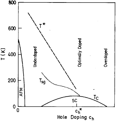
Figure 1: Schematic electronic phase diagram of cuprates

The $T^{*}$ scale [2] shows up clearly as the maximum of the spin susceptibility $\chi_{0}(T=T^{*})$ [3]. The in-plane resistivity $\rho(T)$ is linear $\rho\propto T$ for $T>T^{*}$ and decreases more steeply for $T<T^{*}$. The same $T^{*}$ appears in the anomalous $T$-dependence of the Hall constant $R_{H}(T)$ for $T<T^{*}$ [1]. For the theoretical considerations the most straightforward signature of pseudogap is the reduction of the specific heat coefficient $\gamma=C_{V}/T$ below $T\sim T^{*}$ in the underdoped cuprates [4]. Namely, within normal Fermi liquids $\gamma$ directly measures the quasiparticle (QP) density of states. The spin-gap crossover $T_{sg}$ has been identified in connection with the decrease of the NMR relaxation rate $1/T_{1}$ for $T<T_{sg}$ [1], related to the reduction of low-energy spin excitations. Even more striking is the observation of the leading-edge shift [5] in the angle-resolved photoemission spectroscopy (ARPES) measurements at $T>T_{c}$, a feature interpreted as a $d$-wave SC gap persisting within the normal phase.

It seems to some extent plausible that the $T^{*}$ crossover is related to the onset of short-range antiferromagnetic (AFM) correlations for $T<T^{*}$, since $\chi(T)$ in an undoped AFM has a maximum at $T^{*}\sim 2J/3$ the temperature corresponding to a gradual transition from a disordered paramagnet to the one with short-range AFM correlations. In this contribution we concentrate on our theoretical results which confirm and explain the existence of the pseudogap in the model relevant for cuprates, i.e. the $t$-$J$ model on a 2D square lattice. It should be however pointed out that there there are also several alternative theoretical proposals, which do not directly invoke AFM spin correlations.

The single-particle spectral function $A({\bf k},\omega)$ and its properties are of crucial importance, since their full knowledge would essentially clarify most open questions concerning the anomalous character of strongly correlated electron systems. In recent years there has been an impressive progress in ARPES experiments [5, 6, 1] (in particular for cuprate materials) which in principle yield a direct information on $A({\bf k},\omega)$. In most investigated Bi₂Sr₂CaCu₂O_2+δ (BSCCO) [5] ARPES shows quite a well defined large Fermi surface (FS) in the overdoped and optimally doped samples at $T>T_{c}$, whereby the low-energy behavior with increasing doping in the overdoped regime qualitatively approaches (but does not in fact reach) that of the normal Fermi-liquid with underdamped quasiparticle (QP) excitations. On the other hand, in the underdoped BSCCO QP dispersing through the Fermi surface (FS) are resolved by ARPES only in parts of the large FS, in particular along the nodal $(0,0)$-$(\pi,\pi)$ direction [7, 5], indicating that the rest of the large FS is truncated [8], i.e. either fully or effectively gaped. At the same time near the $(\pi,0)$ momentum ARPES reveals a hump at $\sim 100$ meV [7, 5], which is consistent with large pseudogap scale $T^{*}$. Spectral properties for La_2-xSr_xCu₂O₄ (LSCO), as revealed by ARPES [6] appear to some extent different from BSCCO, presumably due to the crucial role of stripe structures in the LSCO in the regime of intermediate doping. Still they again reveal a truncated FS at low-doping and even the existence of QP along the nodal direction.

The prototype single-band model relevant for cuprates which takes explicitly into account strong correlations is the $t$-$J$ model, derived originally by Chao, Spałek and Oleś [9]

$$H=-\sum_{i,j,s}t_{ij}\tilde{c}^{\dagger}_{js}\tilde{c}_{is}+J\sum_{\langle ij\rangle}({\bf S}_{i}\cdot{\bf S}_{j}-\frac{1}{4}n_{i}n_{j}),$$ (1)

where fermionic operators are projected ones not allowing for the double occupancy of sites, i.e.,

$$\tilde{c}^{\dagger}_{is}=(1-n_{i,-s})c^{\dagger}_{is}.$$ (2)

Longer range hopping appears to be important for the proper description of spectral function in cuprates, in particular it is invoked to explain the difference between electron-doped and hole-doped materials both in the shape of the FS at optimum doping materials [10] as well as for the explanation of the ARPES of undoped insulators [11, 10], we consider besides $t_{ij}=t$ for the n.n. hopping also $t_{ij}=t^{\prime}$ for the n.n.n. hopping on a square lattice. Note that $t^{\prime}<0$ for the hole-doped cuprates.

There have been so far numerous theoretical studies of the $t$-$J$ model on square lattice and related Hubbard model at large Coulomb repulsion $U\gg t$ , as relevant to cuprates, using both analytical approaches as well as numerical techniques for finite size systems. Still analytical approximations to spectral properties have proved to be very delicate, in particular with respect to the question of the emerging pseudogap at lower doping. So there are much fewer studies which give some answers on latter questions within microscopic models close to cuprates. The importance of AFM spin correlations for the emergence of the (large) pseudogap is found in the numerical studies [12, 13, 14] and in phenomenological model studies [15]. The renormalization group studies of the Hubbard model [16] also reveal the instability of the normal Fermi liquid close to the half-filled band (insulator) and a possible truncation of the Fermi surface.

In the following we describe some evidence for the pseudogap within the $t$-$J$ model obtained via finite-size studies and a novel approach to spectral functions using the method of equations of motion.

2 Evidence for the pseudogap from numerical studies

We introduced some years ago a numerical method, i.e. the finite-temperature Lanczos method (FTLM) [17, 14], which is particularly useful for studying finite-size model systems of correlated electrons at $T>0$. The technical advantage of the method is that it is comparable in efficiency to ground state calculations. $T>0$ results for static and dynamical quantities are of interest in themselves, allowing to follow the $T$-variation of properties whereby some of them are meaningful only at $T>0$, e.g. the entropy, the specific heat, the d.c.resistivity etc. On the other hand, the usage of finite but small $T>0$ represents a proper approach to more reliable ground state calculations in small systems.

Figure 2: Uniform susceptibility $\chi_{0}(T)$ at several hole doping $c_{h}$. Results are for $J/t=0.3$.

The most straightforward evidence for a pseudogap within the planar $t$-$J$ model allowing the comparison with experiments appears in the uniform static spin-suceptibility $\chi_{0}(T)$ [18, 14]. Results for various hole concentrations $c_{h}=N_{h}/N$ in a system with $N=20$ sites are presented in Fig. 2. It is evident that the maximum $T^{*}$ being related to the AFM exchange $T^{*}\sim 2J/3$ in an undoped AFM gradually shifts down with doping and finally disappears at ’critical’ $c_{h}=c_{h}^{*}\sim 0.15$. Obtained results are qualitatively as well as quantitatively consistent with experiments in cuprates, e.g. LSCO [3].

Figure 3: The DOS ${\cal N}(\mu+\omega)$ at various $T\leq J$ for hole doping: a) $c_{h}=1/20$ and b) $c_{h}=2/18$.

Another quantity relevant for comparison with the analytical approach further on is the single-particle density of states (DOS) ${\cal N}(\omega)$ [13, 14]. We present in Fig. 3 numerical results for DOS [19] as a function of $T$ for systems with $N=18,20$ sites and two lowest nonzero meaningful hole concentrations $c_{h}\sim 0.05,0.11$. At smallest $c_{h}=0.05$ there is a pronounced pseudogap at $\omega\sim 0$ which closes with increasing $T\sim T^{*}\sim J$. This again indicates the relation of this pseudogap with the AFM short-range correlations which dissolve for $T>J$. On the other hand, the pseudogap closes also on increasing doping since it becomes barely visible at $c_{h}\sim 0.11$.

3 Spectral functions: Equation-of-motion approach

In our analytical approach we analyze the electron Green’s function directly for projected fermionic operators [20, 21],

$$G({\bf k},\omega)=\langle\!\langle\tilde{c}_{{\bf k}s};\tilde{c}^{\dagger}_{{\bf k}s}\rangle\!\rangle_{\omega}=-i\int_{0}^{\infty}{\rm e}^{i(\omega+\mu)t}\langle\{\tilde{c}_{{\bf k}s}(t),\tilde{c}^{\dagger}_{{\bf k}s}\}_{+}\rangle{\rm d}t,$$ (3)

which is equivalent to the usual propagator within the allowed basis states of the model. In the EQM method [22] one uses relations for general correlation functions

$$\omega\langle\!\langle A;B\rangle\!\rangle_{\omega}=\langle\{A,B\}_{+}\rangle+\langle\!\langle[A,H];B\rangle\!\rangle_{\omega}$$ (4)

applying them to the propagator $G({\bf k},\omega)$ [20, 21] one can represent the latter in the form

$$G({\bf k},\omega)=\frac{\alpha}{\omega+\mu-\zeta_{\bf k}-\Sigma({\bf k},\omega)},$$ (5)

where $\alpha$,$\zeta_{\bf k}$ can be expressed in terms of commutators. It is important to notice that the renormalization $\alpha<1$ is already the consequence of the projected basis,

$$\alpha=\frac{1}{N}\sum_{i}\langle\{\tilde{c}_{is},\tilde{c}^{\dagger}_{is}\}_{+}\rangle=\frac{1}{2}(1+c_{h}),$$ (6)

while $\zeta_{\bf k}$ represents the ’free’ propagation emerging from EQM,

$$\zeta_{\bf k}=\frac{1}{\alpha}\langle\{[\tilde{c}_{{\bf k}s},H],\tilde{c}^{\dagger}_{{\bf k}s}\}_{+}\rangle-\bar{\zeta}=-4\eta_{1}t\gamma_{\bf k}-4\eta_{2}t^{\prime}\gamma^{\prime}_{\bf k},$$ (7)

where $\eta_{j}=\alpha+\langle{\bf S}_{0}\!\cdot\!{\bf S}_{j}\rangle/\alpha$ and $\gamma_{\bf k}=(\cos k_{x}+\cos k_{y})/2$, $\gamma_{\bf k}^{\prime}=\cos k_{x}\cos k_{y}$.

The central quantity for further consideration is the self energy

$$\Sigma({\bf k},\omega)=\langle\!\langle C_{{\bf k}s};C^{+}_{{\bf k}s}\rangle\!\rangle_{\omega}^{\rm irr}/\alpha,\qquad iC_{{\bf k}s}=[\tilde{c}_{{\bf k}s},H]-\zeta_{\bf k}\tilde{c}_{{\bf k}s},$$ (8)

and only the ’irreducible’ part of the correlation function should be taken into account in the evaluation of $\Sigma$. EQM enter in the evaluation of $\zeta_{\bf k}$ but even more important in $C_{{\bf k}s}$. We express the commutator in variables appropriate for a paramagnetic metallic state with $\langle{\bf S}_{i}\rangle=0$, and we get

$$[\tilde{c}_{{\bf k}s},H] = [(1-\frac{c_{e}}{2})\epsilon^{0}_{\bf k}-Jc_{e}]\tilde{c}_{{\bf k}s}+$$ (9)

$$+\frac{1}{\sqrt{N}}\sum_{\bf q}m_{\bf kq}\bigl{[}sS^{z}_{\bf q}\tilde{c}_{{\bf k}-{\bf q},s}+S^{\mp}_{\bf q}\tilde{c}_{{\bf k}-{\bf q},-s}-\frac{1}{2}\tilde{n}_{\bf q}\tilde{c}_{{\bf k}-{\bf q},s}\bigr{]},$$

where $\epsilon^{0}_{\bf k}=-4t\gamma_{\bf k}-4t^{\prime}\gamma^{\prime}_{\bf k}$ is the bare band energy, $\tilde{n}_{i}=n_{i}-c_{e}$ and $m_{\bf kq}$ is an effective spin-fermion coupling,

$$m_{\bf kq}=2J\gamma_{\bf q}+\epsilon^{0}_{{\bf k}-{\bf q}}.$$ (10)

One important achievement of the EQM approach is that it naturally leads to an effective coupling (not directly evident within the $t$-$J$ model) between fermionic and spin degrees of freedom, which are essential for proper description of low-energy physics in cuprates. Such a coupling is e.g. assumed in phenomenological models as the spin-fermion model [23, 15]. The essential difference in our case is that $m_{\bf kq}$ is strongly dependent on ${\bf k}$ and ${\bf q}$ just in the vicinity of most relevant ’hot’ spots.

4 Self energy

4.1 Undoped AFM and short range AFM fluctuations

It is quite helpful observation that in the case of an undoped AFM our treatment of $\Sigma$ and the spectral function reproduces quite successful SCBA equations [24] for the Green’s function of a hole in an AFM. If we write EQM in the coordinate space for $\tilde{c}_{is}$ assuming the Néel state as the reference $n_{is}=\pm 1$, we get by considering only the $t$ term,

$$i\frac{d}{dt}\tilde{c}_{is}\sim-t\sum_{j~{}n.n.i}(S^{\mp}_{i}+S^{\mp}_{j})\tilde{c}_{j,-s},$$ (11)

where we have also formally replaced $\tilde{c}_{js}=\tilde{c}_{j,-s}S^{\mp}_{j}$. We note the similarity of Eq. (11) to the effective spin-holon coupling within the SCBA approach. So we can follow the procedure of the evaluation of $\Sigma_{\rm AFM}({\bf k},\omega)$ within the SCBA in the linearized magnon theory [24]

$$\Sigma_{\rm AFM}({\bf k},\omega)=\frac{1}{N}\sum_{\bf q}M_{\bf kq}^{2}G({\bf k}-{\bf q},\omega+\omega_{\bf q}),$$ (12)

where $\omega_{\bf q}$ is the magnon dispersion and $M_{\bf kq}=4t(u_{\bf q}\gamma_{{\bf k}-{\bf q}}+v_{\bf q}\gamma_{\bf k})$ is the holon-magnon coupling which in general strong $\propto t$, but vanishes near the AFM wavevector ${\bf q}={\bf Q}=(\pi,\pi)$.

The advantage of the representation of EQM, Eq. (11), explicitly in spin and fermionic variables is that it allows the generalization to finite doping $c_{h}>0$. We assume that spin fluctuations remain dominant at the AFM wavevector ${\bf Q}$ with the characteristic inverse AFM correlation length $\kappa=1/\xi_{AFM}$. The latter seems to be the case for BSCCO as well as YB₂Cu₃O_6+x, but not for LSCO with pronounced stripe and spin-density structures [1]. For BSCCO and YBCO it is sensible to divide the spin fluctuations into two regimes with respect to $\tilde{\bf q}={\bf q}-{\bf Q}$: a) For $\tilde{q}>\kappa$ spin fluctuations are paramagnons, they are propagating like magnons and are transverse to the local AFM short-range spin. b) For $\tilde{q}<\kappa$ spin fluctuations are essentially not propagating modes but critically overdamped so deviations from the long range order are essential.

At finite doping case we therefore generalize (at $T=0$) Eq. (19) into the paramagnon contribution,

$$\Sigma_{\rm pm}({\bf k},\omega)=\!\frac{1}{N}\!\!\!\sum_{q,\tilde{q}>\kappa}\bigl{[}M_{\bf kq}^{2}G^{-}({\bf k}-{\bf q},\omega+\omega_{\bf q})+M_{{\bf k}+{\bf q},{\bf q}}^{2}G^{+}({\bf k}+{\bf q},\omega-\omega_{\bf q})],$$ (13)

where $G^{\pm}({\bf k},\omega)$ refer to the electron ($\omega>0$) and hole-part ($\omega<0$) of the propagator, respectively. We are dealing in Eq. (13) with a strong coupling theory due to $t>\omega_{\bf q}$ and a selfconsistent calculation of $\Sigma_{\rm pm}$ is required [21]. Also, resulting $\Sigma_{\rm pm}({\bf k},\omega)$ and $A({\bf k},\omega)$ as are at low doping quite asymmetric with respect to $\omega=0$, since $G^{-}\propto(1-c_{h})/2\sim 1/2$ while $G^{+}\propto c_{h}$.

4.2 Longitudinal spin fluctuations

At $c_{h}>0$ the electronic system is in a paramagnetic state without an AFM long-range order and besides the paramagnon excitations also the coupling to longitudinal spin fluctuations become crucial. The latter restore the spin rotation symmetry in a paramagnet and EQM (9) introduce such a spin-symmetric coupling. Within a simplest approximation that the dynamics of fermions and spins is independent, we get

$$\Sigma_{\rm lf}({\bf k},\omega)=\frac{1}{\alpha}\sum_{\bf q}\tilde{m}^{2}_{\bf kq}\int\!\!\int\frac{{\rm d}\omega_{1}{\rm d}\omega_{2}}{\pi}g(\omega_{1},\omega_{2})\frac{\tilde{A}({{\bf k}-{\bf q}},\omega_{1})\chi^{\prime\prime}({\bf q},\omega_{2})}{\omega-\omega_{1}-\omega_{2}},$$ (14)

where $g(\omega_{1},\omega_{2})=(1/2)[{\rm th}(\beta\omega_{1}/2)+{\rm cth}(\beta\omega_{2}/2)]$ and $\chi$ is the dynamical spin susceptibility. Quite analogous treatment has been employed previously in the Hubbard model [25] and more recently within the spin-fermion model [15, 26].

If we want to use the analogy with the spin-fermion Hamiltonian the effective coupling parameter $\tilde{m}_{\bf kq}$ should satisfy $\tilde{m}_{{\bf k},{\bf q}}=\tilde{m}_{{\bf k}-{\bf q},-{\bf q}}$ which is in general not the case with the form Eq. (10), therefore we use further on instead the symmetrized coupling

$$\tilde{m}_{\bf kq}=2J\gamma_{\bf q}+\frac{1}{2}(\epsilon^{0}_{{\bf k}-{\bf q}}+\epsilon^{0}_{\bf k}).$$ (15)

In contrast to previous related studies of spin-fermion coupling [25, 15, 26], however, $\tilde{m}_{\bf kq}$ is strongly dependent on both ${\bf q}$ and ${\bf k}$. It is essential that in the most sensitive parts of the FS, i.e., along the AFM zone boundary (’hot’ line) where $k=|{\bf Q}-{\bf k}|$, the coupling is in fact quite modest determined solely by $J$ and $t^{\prime}$. Also, in the regime close to that of quasistatic $\chi({\bf q},\omega)$ the simplest and also quite satisfactory approximation is to insert for $\tilde{A}$ the unrenormalized $A^{0}$ [15], the latter corresponding in our case to the spectral function without $\Sigma_{\rm lf}$ but with $\Sigma=\Sigma_{\rm pm}$.

In the present theory spin susceptibility $\chi({\bf q},\omega)$ is taken as an input. The system is close to the AFM instability, so we assume spin fluctuations of the overdamped form [23]

$$\chi^{\prime\prime}({\bf q},\omega)\propto\frac{\omega}{(\tilde{q}^{2}+\kappa^{2})(\omega^{2}+\omega_{\kappa}^{2})}.$$ (16)

Nevertheless, the appearance of the pseudogap and the form of the FS are not strongly sensitive to the particular form of $\chi^{\prime\prime}({\bf q},\omega)$ at given characteristic $\kappa$ and $\omega_{\kappa}$.

5 Pseudogap

We first establish some characteristic features of the pseudogap and the development of the FS following a simplified analysis. We note that $\Sigma_{\rm pm}$ induces a large incoherent component in the spectral functions at $\omega\ll 0$ and renormalizes the effective QP band relevant to the behavior at $\omega\sim 0$ and at the FS [21]. It can also lead to a transition of a large FS into a small hole-pocket-like FS at very small $c_{h}<c_{h}^{*}\ll 1$. Nevertheless, the pseudogap can appear only via $\Sigma_{\rm lf}$. Therefore we here take into account $\Sigma_{\rm pm}$ only via an effective band $\epsilon_{\bf k}^{\rm ef}$. The input spectral function for $\Sigma_{\rm lf}$ is thus

$$A^{0}_{\rm ef}({\bf k},\omega)=\alpha Z^{\rm ef}_{\bf k}\delta(\omega+\mu-\epsilon_{\bf k}^{\rm ef}).$$ (17)

We restrict our discussion to $T=0$ and to the regime of intermediate (not too small) doping, where $\epsilon_{\bf k}^{\rm ef}$ defines a large FS. The simplest case is the quasi-static and single-mode approximation (QSA) which is meaningful if $\omega_{\kappa}\ll t,\kappa\ll 1$, where we get

$$G^{QSA}({\bf k},\omega)=\frac{\alpha Z^{\rm ef}_{\bf k}(\omega-\epsilon^{\rm ef}_{{\bf k}-{\bf Q}})}{(\omega-\epsilon^{\rm ef}_{{\bf k}-{\bf Q}})(\omega-\epsilon^{\rm ef}_{\bf k})-\Delta^{2}_{\bf k}}.$$ (18)

The spectral function shows in this approximation two branches of $E^{\pm}$, separated by the gap which opens along the AFM zone boundary ${\bf k}={\bf k}_{AFM}$ and the relevant (pseudo)gap scale is

$$\Delta^{PG}_{\bf k}=|\Delta_{{\bf k}_{AFM}}|=\frac{Z^{\rm ef}_{\bf k}}{2}\sqrt{r_{s}}|2J-4t^{\prime}{\rm cos}^{2}k_{x}|.$$ (19)

$\Delta^{PG}_{\bf k}$ does not depend on $t$, but rather on smaller $J$ and in particular $t^{\prime}$. For $t^{\prime}<0$ the gap is largest at $(\pi,0)$, consistent with experiments [7, 5].

QSA yileds a full gap corresponding, e.g., to the case of a long-range AFM state. Within the simplified effective band approach, Eq. (17), it is not difficult to evaluate numerically $\Sigma_{\rm lf}$ beyond the QSA, by taking explicitly $\chi^{\prime\prime}({\bf q},\omega)$, Eq. (16), with $\kappa>0$ and $\omega_{\kappa}\sim 2J\kappa$. For illustration, we present results characteristic for the development of spectral functions varying two most sensitive parameters $\kappa$ and $\mu$, which both simulate the variation with doping, e.g. one can $\kappa$ take in accordance with experiments [1] and numerical results on the $t$-$J$ model [27] as $\kappa\sim\sqrt{c_{h}}$.

In Fig. 3 we present results for $A({\bf k},\omega=0)$ at $T=0$ for a broad range of $\kappa=0.01-0.6$. Curves in fact display the effective FS determined by the condition $G^{-1}({\bf k}_{F},0)\sim 0$. At the same time, intensities $A({\bf k},\omega=0)$ correspond to the QP weight $Z_{F}$ at the FS. At very small $\kappa=0.01$ we see a small (hole-pocket) FS which follows from the QSA, Eq. (18). Already $\kappa\sim 0.05$ destroys the ’shadow’ side of the pocket, i.e., the solution $G^{-1}=0$ on the latter side disappears. On the other hand, in the gap emerge now QP solutions with very weak $Z_{F}\ll 1$ which reconnect the FS into a large one. We are dealing nevertheless with effectively truncated FS with well developed arcs. The effect of larger $\kappa$ is essentially to increase $Z_{F}$ in the gapped region, in particular near $(\pi,0)$. Finally, for large $\kappa=0.6$ corresponding in cuprates to the optimal doping or overdoping, $Z_{F}$ is essentially only weakly decreasing towards $(\pi,0)$ and the FS is well pronounced and concave as naturally expected for $t^{\prime}<0$.

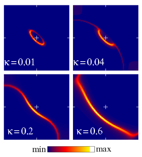
Figure 4: Contour plot of spectral functions $A({\bf k},\omega=0)$ at $T=0$ for various $\kappa$ in one quarter of the Brillouin zone.

We note in Fig. 4 that except at extreme $\kappa=0.01$ we get a large FS, whereby in the ’underdoped’ regime $\kappa<\kappa^{*}\sim 0.5$ the QP weight $Z_{F}$ is substantial only within pronounced ’arcs’ and very small along the ’gapped’ FS where $Z_{F}\ll 1$. Still, such a situation corresponds to a Fermi liquid, although a very strange one, where QP excitations exist everywhere along the FS and hence determine the low-energy properties of the ’normal’ metallic state.

It is quite remarkable to notice that in spite of $Z_{F}\ll 1$ the QP velocity $v_{F}$ is not diminished within the pseudogap. In fact it can be even enhanced, as seen in in Fig. 5 where the contour plot of $A({\bf k},\omega)$ is shown. Again, it is well evident in Fig. 5 that QP is well defined at the FS, while it becomes fuzzy at $\omega\neq 0$ merging with the solutions $E_{\bf k}^{\pm}$, respectively, away from the FS. The effect of large $v_{F}$ in the pseudogap, which is essential for the low-$T$ thermodynamics, can be only explained with a crucial ${\bf k}$ dependence of $\Sigma$. Assuming that ${\bf k}$ enters only via $\epsilon({\bf k})$ we can express $v_{F}$ renormalization as

$$\frac{v_{F}}{v^{\rm ef}_{\bf k}}=(1+\frac{\partial\Sigma^{\prime}}{\partial\epsilon})\frac{Z_{F}}{Z^{\rm ef}},\qquad\frac{\partial\Sigma^{\prime}}{\partial\epsilon}\Bigr{|}_{\omega=0}\sim\frac{\Delta^{2}}{w(\omega_{\kappa}+w)}.$$ (20)

While $Z_{F}/Z^{ef}\ll 1$ in the same case, $\partial\Sigma^{\prime}/\partial\epsilon$ compensates or even leads to an enhancement of $v_{F}$. In the case $\omega_{\kappa}w\ll\Delta^{2}$ we get

$$\frac{v_{F}}{v^{\rm ef}_{\bf k}}\sim\frac{\omega_{\kappa}}{w}\sim\frac{2J}{v_{\bf k}}.$$ (21)

Final $v_{F}$ is therefore not strongly renormalized, since $2J$ and $v^{\rm ef}_{\bf k}$ are of similar order. Furthermore, $v_{F}$ is enhanced in the parts of FS where $v^{\rm ef}_{\bf k}$ is small, in particular near $(\pi,0)$ point. The situation is thus very different from ’local’ theories where $\Sigma({\bf k},\omega)\sim\Sigma(\omega)$ and the QP velocity is governed only by $Z_{F}$. In our case the ’nonlocal’ character of $\Sigma({\bf k},\omega)$ is essential in order to properly describe QP within the pseudogap region.

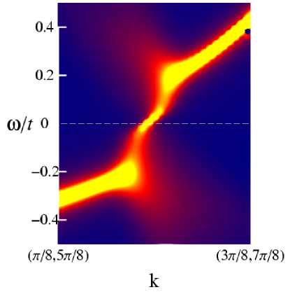
Figure 5: Contour plot of spectral functions $A({\bf k},\omega=0)$ across the FS in the pseudogap regime.

¿From $A({\bf k},\omega)$ we can calculate the DOS ${\cal N}(\omega)=(2/N)\sum_{\bf k}A({\bf k},\omega)$. At the Fermi energy $\omega\sim 0$ and low $T$ one can express the DOS also as (assuming the existence of QP around the FS),

$${\cal N}(0)\sim\frac{\alpha}{2\pi^{2}}\oint\frac{{\rm d}S_{F}Z({\bf k}_{F})}{v({\bf k}_{F})}.$$ (22)

The contribution will come mostly from FS arcs near the zone diagonal while the gapped regions near $(\pi,0)$ will contribute less due to $Z({\bf k}_{F})\ll 1$. Results in Fig. 6(a) show the development of ${\cal N}(0)$ with $\kappa$. As expected the DOS decreases with decreasing $\kappa$ simulating the approach to an undoped AFM. The DOS is measured in cuprates via angle integrated photoemission spectroscopy, e.g. for LSCO in [28], as well as via the scanning tunneling microscopy (STM) [29]. Our results are qualitatively consistent with these experiments (showing ${\cal N}(0)$ scaling with doping) as well as with numerical results on the $t$-$J$ model [13, 14], as shown in Fig. 3. It is well possible that within photoemission experiments the matrix elements are essential, so we present in Fig. 6(a) also results weighted by the matrix element $w({\bf k})=(\cos k_{x}-\cos k_{y})^{2}$, which originates from the interplanar hopping as proposed for the $c$-axis conductivity [30]. Such weighted results show a stronger dependence on doping due to enhanced influence of the pseudogap region near $(\pi,0)$, which could be even closer to experimental findings [28]. In Fig. 6(b) we show also the average $Z_{\rm av}$ along the FS, as well as the QP DOS, defined as

$${\cal N}_{QP}=\frac{1}{2\pi^{2}}\oint\frac{{\rm d}S_{F}}{v({\bf k})}.$$ (23)

The decrease $Z_{\rm av}$ has similar dependence at the DOS ${\cal N}(0)$. It is however quite important to notice that smaller doping (decreasing $\kappa$) leads also to a decrease of ${\cal N}_{QP}$. This is consistent with the observation of the pseudogap also in the specific heat in cuprates [4], since ${\cal N}_{QP}\propto\gamma=C_{V}/T$. We note here that such a behavior is not at all evident in the vicinity of a metal-insulator transition [1]. Namely, in a Fermi liquid with (nearly constant) large FS one can drive the metal-insulator transition by $Z_{\rm av}\to 0$. Within an assumption of a local character $\Sigma(\omega)$ this would also lead to $v_{F}\to 0$ and consequently via Eq. (23) to ${\cal N}_{QP}\to\infty$. Clearly, the essential difference in our case is that within the pseudogap regime $\Sigma({\bf k},\omega)$ is nonlocal, allowing for a large (not reduced or even enhanced) velocity within the pseudogap regime, hence a simultaneous decrease of ${\cal N}(0)$ and ${\cal N}_{QP}$.

Figure 6: (a) DOS ${\cal N}(0)$ and weighted DOS ${\cal N}_{\rm w}(0)$ vs. $\kappa$. (b) Average QP weight $Z_{\rm av}$ and QP DOS ${\cal N}_{\rm QP}$ vs. $\kappa$.

It is also important to understand the role of finite $T>0$. The most pronounced effect is on QP in the pseudogap part of the FS. The main conclusion is that weak QP peak with $Z_{F}\ll 1$ at $T=0$, as seen e.g. in Fig. 5, is not just broadened but entirely disappears (becomes incoherent) already at very small $T>T_{s}\ll J$, e.g. $T_{s}\sim 0.02~{}t$ for the situation in Fig. 5. This can explain the puzzle that ARPES experiments in fact do not observe any QP peak near $(\pi,0)$ in the underdoped regime at $T>T_{c}$ [7, 5].

6 Conclusions

In this paper we have presented our results for spectral functions and the pseudogap within the $t$-$J$ model, which is the prototype model for strongly correlated electrons and for superconducting cuprates in particular. Here we first comment on the validity of the model and results in a broader perspective of strange metals and materials close to the metal-insulator transition. The physics of the $t$-$J$ model at lower doping levels is determined by the interplay between the magnetic exchange (dominating the undoped AFM insulator) and the itinerant kinetic energy of fermions (being dominant at least in the overdoped regime). Since itinerant fermions prefer a ferromagnetic state, the quantum state at the intermediate doping is frustrated, the quantum frustration showing up in large entropy, pronounced spin fluctuations, non-Fermi liquid effects etc. Evidently, this is one path towards the metal-insulator transition, but definitely not the only one possible. In this situation, fermionic and spin degrees of freedom are coupled but both active and relevant for low-energy properties. This is just the main content and assumption of the presented theory for spectral functions and the pseudogap.

The EQM approach to dynamical properties seem to be promising since it can treat exactly the constraint which is essential for the physics of strongly correlated electrons. It has been recently also applied by present authors to the analysis of spin fluctuations and collective magnetic modes at low $T$. Our approximation for the self energy within the EQM approach deals with the normal paramagnetic state and treats the model as a coupled system (with derived effective coupling) of fermions with spin fluctuations, where close to the AFM ordered state both transverse and longitudinal spin fluctuations are important. Other contributions should be considered, e.g., the coupling to pairing fluctuations, in order to treat the superconducting state.

In this paper we present only the results of the simplified pseudogap analysis. The results of full self-consistent treatment are qualitatively similar [21]. Within the present theory the origin of the pseudogap feature is in the coupling to longitudinal spin fluctuations near the AFM wavevector ${\bf Q}$ which determine the QP properties in the ’hot’ region, i.e. near the AFM zone boundary. The pseudogap opens predominantly in the same region and its extent is dependent on $J$ and $t^{\prime}$ but not directly on $t$. Evidently the pseudogap bears a similarity to a d-wave-like dependence along the FS (for $t^{\prime}<0$) being largest near the $(\pi,0)$ point. The strength of the pseudogap features depends mainly on $\kappa$. It is important to note that apart from extremely small $\kappa$ we are still dealing with a large FS. Still, at $\kappa<\kappa^{*}\sim 0.5$ parts of the FS near $(\pi/2,\pi/2)$ remain well pronounced while the QP weight within the pseudogap part of the FS are strongly suppressed, in particular near zone corners $(\pi,0)$.

The QP within the pseudogap have small weight $Z_{F}\ll 1$ but not diminished (or even enhanced) $v_{F}$, which is the effect of the nonlocal character of $\Sigma({\bf k},\omega)$. A consequence is that QP within the pseudogap contribute much less to QP DOS ${\cal N}_{QP}$. This could be plausible explanation of a well known theoretical challenge that approaching the magnetic insulator both DOS, i.e. ${\cal N}(0)$ and ${\cal N}_{QP}$ vanish.

We presented results for $T=0$, however the extention to $T>0$ is straightforward. Discussing only the effect on the pseudogap, we notice that it is mainly affected by $\kappa$. So we can argue that the pseudogap should be observable for $\kappa(c_{h},T)<\kappa^{*}\sim 0.5$. This effectively determines the crossover temperature $T^{*}(c_{h})$. In the region of interest $\kappa$ is nearly linear in both $T$ and $c_{h}$ so we would get approximately

$$T^{*}\sim T^{*}_{0}(1-c_{h}/c_{h}^{*}),$$ (24)

where $T^{*}_{0}\sim 0.6J$ and $c_{h}^{*}\sim 0.15$.

As described in previous sections, several features of our theory, regarding the development of spectral functions, Fermi surface and pseudogap, are at least qualitatively consistent with experimental results of normal state properties in cuprates. However, further study within the present formalism is necessary in order to explore possible closer quantitative agreement with experiments as well as the emergence of superconductivity within the same model.

References

- [1] for a review see, e.g., M. Imada, A. Fujimori, and Y. Tokura, Rev. Mod. Phys. 70, 1039 (1998).
- [2] B. Batlogg et al., Physica C 235 - 240, 130 (1994).
- [3] D. C. Johnston et al., Phys. Rev. Lett. 62, 957 (1989); J. B. Torrance et al., Phys. Rev. B 40, 8872 (1989).
- [4] J.W. Loram, K.A. Mirza, J.R. Cooper, and W.Y. Liang, Phys. Rev. Lett. 71, 1740 (1993); J.W. Loram, J.L. Luo, J.R. Cooper, W.Y. Liang, and J.L. Tallon, Physica C 341 - 8, 831 (2000).
- [5] J.C. Campuzano and M. Randeria et al., in Proc. of the NATO ARW on Open Problems in Strongly Correlated Electron Systems, Eds. J. Bonča, P. Prelovšek, A. Ramšak, and S. Sarkar (Kluwer, Dordrecht, 2001), p. 3.
- [6] A. Fujimori et al., in Proc. of the NATO ARW on Open Problems in Strongly Correlated Electron Systems, Eds. J. Bonča, P. Prelovšek, A. Ramšak, and S. Sarkar (Kluwer, Dordrecht, 2001), p. 119.
- [7] D.S. Marshall et al., Phys. Rev. Lett. 76, 4841 (1996); H. Ding et al., Nature 382, 51 (1996).
- [8] M.R. Norman et al., Nature 392, 157 (1998).
- [9] K.A. Chao, J. Spałek and A.M. Oleś, J. Phys.C 10, L271 (1977).
- [10] T. Tohyama and S. Maekawa, J. Phys. Soc. Jpn. 59, 1760 (1990).
- [11] B. O. Wells et al., Phys. Rev. Lett. 74, 964 (1995).
- [12] R. Preuss, W. Hanke, C. Gröber, and H.G. Evertz, Phys. Rev. Lett. 79, 1122 (1997).
- [13] J. Jaklič and P. Prelovšek, Phys. Rev. B 55, R7307 (1997); P. Prelovšek, J. Jaklič, and K. Bedell, Phys. Rev. B 60, 40 (1999).
- [14] for a review see J. Jaklič and P. Prelovšek, Adv. Phys. 49, 1 (2000).
- [15] A.V. Chubukov and D.K. Morr, Phys. Rep. 288, 355 (1997).
- [16] D. Zanchi and H.J. Schulz, Europhys. Lett. 44, 235 (1997); N. Furukawa, T.M. Rice, and M. Salmhofer, Phys. Rev. Lett. 81, 3195 (1998).
- [17] J. Jaklič and P. Prelovšek, Phys. Rev. B 49, 5065 (1994).
- [18] J. Jaklič and P. Prelovšek, Phys. Rev. Lett. 77, 892 (1996).
- [19] P. Prelovšek, A. Ramšak, and I. Sega Phys. Rev. Lett. 81, 3745 (1998).
- [20] P. Prelovšek, Z. Phys. B 103, 363 (1997).
- [21] P. Prelovšek and A. Ramšak, Phys. Rev. B 63, 180506 (2001); ibid. 65, 174529 (2002).
- [22] D. N. Zubarev, Sov. Phys. Usp. 3, 320 (1960).
- [23] P. Monthoux, A.V. Balatsky, and D. Pines, Phys. Rev. Lett. 67, 3448 (1991); P. Monthoux and D. Pines, Phys. Rev. B 47, 6069 (1993).
- [24] C.L. Kane, P.A. Lee, and N. Read, Phys. Rev. B 39, 6880 (1989); G. Martínez and P. Horsch, ibid. 44, 317 (1991); A. Ramšak and P. Prelovšek, ibid. 42, 10415 (1990).
- [25] A. Kampf and J.R. Schrieffer, Phys. Rev. B 41, 6399 (1990).
- [26] J. Schmalian, D. Pines, and B. Stojković, Phys. Rev. Lett. 80, 3839 (1998); Phys. Rev. B 60, 667 (1999).
- [27] For a review, see E. Dagotto, Rev. Mod. Phys. 66, 763 (1994).
- [28] A. Ino et al., Phys. Rev. Lett. 81, 2124 (1998).
- [29] Ch. Renner, B. Revaz, K. Kadowaki, I. Maggio-Aprile, and O. Fischer, Phys. Rev. Lett. 80, 3606 (1998).
- [30] L.B. Ioffe and A.J. Millis, Phys. Rev. B 58, 11631 (1998).