Phys. Rev. B 68, 134445 (2003)
Luttinger liquid behavior in spin chains with a magnetic field

Abstract

Antiferromagnetic Heisenberg spin chains in a sufficiently strong magnetic field are Luttinger liquids, whose parameters depend on the actual magnetization of the chain. Here we present precise numerical estimates of the Luttinger liquid dressed charge $Z$, which determines the critical exponents, by calculating the magnetization and quadrupole operator profiles for $S=1/2$ and $S=1$ chains using the density matrix renormalization group method. Critical amplitudes and the scattering length at the chain ends are also determined. Although both systems are Luttinger liquids the characteristic parameters differ considerably.

I Introduction

The one-dimensional (1D) antiferromagnetic Heisenberg chain

$$H=\sum_{i=1}^{N-1}{\rm\bf S}_{i}{\rm\bf S}_{i+1}-h\sum_{i=1}^{N}S^{z}_{i}$$ (1)

is one of the most thoroughly investigated paradigms of interacting many-body systems. It is well-known that for zero magnetic field the low-energy physics depends very much on the spin length $S$. As Haldane predicted in 1983,Hal-gap-83 integer $S$ chains possess an energy gap $\Delta_{g}(S)$ above the ground state, the size of which vanishes exponentially as $S\to\infty$, whereas half-integer $S$ chains are gapless. The presence of the Haldane gap in integer spin chains implies the occurrence of a critical field $h_{c}=\Delta_{g}$ beyond which the system gets magnetized. As the gap collapses at the critical field the ground state structure changes adequately, and in an already magnetized state there remains no conceptual difference in the low-energy properties between integer and half-integer chains.

Partially magnetized antiferromagnetic Heisenberg chains at low energies are expected to be one-component Luttinger liquidsHal-JPC81 (LLs) irrespective of the spin length $S$. This is known rigorously in the $S=1/2$ case where the model can be analyzed using the Bethe Ansatz.Hal-PRL80 The validity of the Luttinger liquid description for $S\geq 1$ chains and coupled spin-1/2 ladders has been investigated and confirmed by analyticalTsvelik ; Chi-Gia ; Kon-Fen and numericalSak-Tak ; Usa-Sug ; Hik-Fur methods. Although there is a theoretical possibility of finding gapful behavior (magnetization plateau) at special values of the magnetization, such a scenario does not seem to be realized in pure nearest-neighbor Heisenberg chains (see Ref. Osh-Yam-Aff, for $S=3/2$). Neither would we expect multi-component LLs, which can otherwise occur for more general (higher-order) couplings.Fat-Lit

The LL concept bears a strong relationship to $c=1$ conformal field theory (CFT).Gog-Ner-Tsv In fact the LL is hardly more than the CFT adapted to the situation with two Fermi points $2k_{F}$ momentum apart. The one-component LL is a three parameter theory.Hal-JPC81 In the present context the first parameter, the location of the Fermi points $\pm k_{F}$, is determined by the magnetization through

$$2k_{F}=2\pi(S-m),$$ (2)

where $m=S^{z}_{\rm tot}/L$ is the (bulk) magnetization. The second parameter, the Fermi velocity $v$ is just an energy scale, whereas the third parameter, to be called the ”dressed charge” $Z$, determines the universality class and the critical exponents. (In the bosonization literature the notation $K=Z^{2}$ is standard.) The traditional LL parameters, the velocities for charge and current excitations can be expressed with $Z$ as $v_{\rm charge}=v/Z^{2}$, $v_{\rm current}=vZ^{2}$.Hal-PRL81

All three parameters are functions of the actual magnetization $m$ and the spin length $S$. The LL parameters of the $S=1$ chain in a magnetic field have already been determined to some extent using numerical methods. Sakai and Takahashi diagonalized small finite chains up to $N=16$ with periodic boundary condition and used the prediction of CFT on finite size energy spectra to estimate the critical exponents.Sak-Tak A similar method was used by Usami and SugaUsa-Sug for the $S=1/2$ ladder which behaves as a Haldane-gap system for strong ferromagnetic interchain interaction. More recently Campos Venuti et al. used the DMRG to compute directly the transverse two-point function $G^{xx}(r)=\langle S^{x}(0)S^{x}(r)\rangle$ on chains with $N=80$ and fitted these data to the expected asymptotic form of $G^{xx}$.Campos-Venuti

In this paper we apply an alternative method. We calculate precise numerical estimates to the critical exponents and by this to the LL dressed charge $Z$ via a direct numerical determination of the magnetization profiles in finite open chains. The magnetization profile is, by definition, the positional dependence of the local magnetization $m_{n}=\langle S^{z}_{n}\rangle$ in an open chain with some well-defined boundary condition. The form of the profile depends on the applied boundary condition, and may involve surface exponents as well whenever the boundary condition on the left and right ends differ. In order to simplify the expected behavior we will only consider cases where the boundary condition is identically open (free) on both ends; in this case only bulk exponents come into play.BurkEise In a semi-infinite chain, far from the chain’s end, the magnetization profile is expected to decay to its bulk value $m$ algebraically as

$$m(r)\simeq m+A_{m}\cos(2k_{F}r+\phi)\,r^{-\eta_{z}/2},$$ (3)

where $A_{m}$ is a non-universal amplitude, $\phi$ is a phase shift, $\eta_{z}$ is the (bulk) critical exponent, defined through the translation invariant longitudinal two-point function $G^{zz}(r)=\langle S^{z}(0)S^{z}(r)\rangle-m^{2}\simeq A\cos(2k_{F}r+\phi)\,r^{-\eta_{z}}$, and $k_{F}$ is determined as a function of $m$ by Eq. (2). The form of the Friedel oscillation in Eq. (3) contains indirect information about the LL parameter $Z$, and this can be exploited in a numerical procedure to calculate precise estimates. This program has been carried out for the $S=1/2$ chain and ladders in Ref. Hik-Fur, , for the Kondo lattice model in Ref. Shibata, , for the Hubbard model in Ref. Bedurftig, , and for the $t-J$ model in Ref. White-Affleck, .

While the algebraic decay with $\eta_{z}/2$ is a standard consequence of criticality,Fis-deG the $2k_{F}$ oscillation is a special LL feature, which stems from the fact that we work with two families of (chiral) CFT operators living around the two Fermi points in $k$-space. Without the $2k_{F}$ oscillation it is a standard exercise in CFT to derive the shape of the magnetization profile in a strip geometry of width $L$ by applying the logarithmic mapping.Cardy ; BurkEise This transformation, together with the proper account for the $2k_{F}$ LL term yields a prediction for the magnetization profile of a finite Luttinger liquid segment of length $L$ with open boundary condition on both endsHik-Fur ; White-Affleck

$$m^{(L)}(r)\simeq m+A_{m}\cos\!\left[2k_{F}\!\!\left(r-\frac{L}{2}\right)\right]\left[{L\over\pi}\sin\!\left(\pi\frac{r}{L}\right)\right]^{-\eta_{z}/2}\!\!\!.$$ (4)

Note that there is no need to introduce explicitly a phase shift $\phi$ as in the semi-infinite case Eq. (3), since the symmetry of the profile with respect to $r\to L-r$ implies that $\phi=-k_{F}L$.

The predicted LL profile in Eq. (4) is based on the continuum limit. However, for finite lattice systems such as the Heisenberg chain, we expect corrections. Conformal invariance and thus Eq. (4) is only expected to be valid asymptotically in the large $L$ limit with $r$ satisfying $0<<r<<L$. Clearly, in a strict sense the magnetization cannot diverge at the chain ends since $m_{n}\leq S$. Phenomenologically this natural cut-off at the boundary acts as an effective impurity put into the CFT model at the system ends. This defines an effective ”scattering length”, $\delta N={\cal O}(1)$, associated with the boundary, suggesting that we should replace the naive system size $L=N$ in Eq. (4) with an ”effective” system size $L\to N+2\,\delta N$. Based on this intuitive argument in the following we will work with a slightly modified Ansatz

$$m^{(N)}_{n}\! \simeq \!m+A_{m}\cos\left[2k_{F}\left(n-{N+1\over 2}\right)\right]$$ (5)

$$\times\left[{N+2\,\delta N\over\pi}\sin\!\left(\pi\frac{n-1/2+\delta N}{N+2\,\delta N}\right)\right]^{-\eta_{z}/2}$$

where $\delta N$ is a free fitting parameter. When $\delta N=0$ Eq. (5) is simply the discrete version of Eq. (4) (note that now the system is defined for $n=1,\dots,N$).

In the lack of a consistent scheme to calculate corrections, the above amendment to the fitting formula is not rigorous. Justification can stem from a direct comparison with exact results. In the following we first discuss in detail the exactly solvable $S=1/2$ chain as a benchmark case. We demonstrate that the Ansatz in Eq. (5) is capable of reproducing the (numerically) exact $S=1/2$ critical exponents to high precision even with $\delta N=0$. When $\delta N$ is also fitter for, the accuracy improves by an order of magnitude.

II The $S=1/2$ chain: Bethe Ansatz results

The $S=1/2$ Heisenberg chain in a magnetic field can be solved exactly by the Bethe Ansatz (BA) method.Grif-Yan-Yan The BA itself cannot yield the correlation functions and critical exponents directly, but assuming conformal invariance the operator content can be read off from the structure of the low-energy excitations above the ground state.Cardy These latter can be determined by a systematic calculation of the finite size corrections to the $L=\infty$ BA equations (assuming periodic boundary condition).Woy-Eck-deVega The energy and momentum of the lowest energy (primary) states (with respect to those of the ground state, $E_{g}$ and $P_{g}$) can be cast into the form

$$\delta E = E_{\bf a}-E_{g}=\frac{2\pi v}{N}(\Delta^{+}+\Delta^{-}),$$ (6)

$$\delta P = P_{\bf a}-P_{g}=Q+\frac{2\pi}{N}(\Delta^{+}-\Delta^{-}),$$ (7)

where ${\bf a}=\{d,l\}$ is a shorthand for two integer topological quantum numbers labeling the states. The ${\cal O}(1)$ momentum term is

$$Q=Q_{\bf a}=2k_{F}d+\pi l,$$ (8)

with $k_{F}$ defined in Eq. (2). The ”conformal dimensions” $\Delta^{\pm}$ read

$$\Delta^{\pm}={1\over 2}\left[Zd\pm\frac{l}{2Z}\right]^{2},$$ (9)

where $Z$ is the dressed charge. The topological quantum numbers have a direct physical interpretation in the LL representation: $l$ ($d$) denotes the number of fermions added to (transferred from the left Fermi point to the right in) the band.

Figure 1: The dressed charge as a function of the magnetization in an $S=1/2$ chain; $\diamond$ denotes results using the naive fit $\delta N=0$, $+$ denotes fits where $\delta N$ is optimized. Solid line is the Bethe Ansatz result. Inset shows the critical exponents and the numerically determined amplitude $A_{m}$. At $m=0$ the dressed charge is $Z=1/\sqrt{2}$.

The critical exponents appearing in the one- and two-point correlation functions can be expressed with the conformal dimensions $\Delta^{\pm}$. In general a physical operator such as $S^{z}$ decomposes into all operators which are not forbidden by conservation (selection) rules. In particular, for $S^{z}$ the number of fermions in the band is conserved, thus necessarily $l=0$. The asymptotic decay is determined by the operator which has the lowest critical exponent, i.e., $d=1$ giving

$$\eta_{z}=\left.2(\Delta^{+}+\Delta^{-})\right|_{l=0,d=1}=2Z^{2},$$ (10)

and an oscillation $2k_{F}$ by Eq. (8). The transverse critical exponents $\eta_{x}$ is determined by the operator $l=1,d=0$, i.e.,

$$\eta_{x}=\left.2(\Delta^{+}+\Delta^{-})\right|_{l=1,d=0}=\frac{1}{2Z^{2}},$$ (11)

with the associated oscillation frequency $Q=\pi$. Equations (10) and (11) imply $\eta_{z}\eta_{x}=1$.

In the BA approach the dressed charge $Z=Z(B)$ is determined by a set of integral equations for the density of rapidities $\rho(x)$, and the dressed charge function $Z(x)$,Par-Schm-Cab

$$\rho(x) = g(x)+\int_{-B}^{B}K(x-x^{\prime})\rho(x^{\prime})dx^{\prime},$$ (12)

$$Z(x) = 1+\int_{-B}^{B}K(x-x^{\prime})Z(x^{\prime})dx^{\prime},$$ (13)

where

$$g(z)=\frac{1}{\pi(1+z^{2})},\qquad K(z)=\frac{-2}{\pi(4+z^{2})}.$$ (14)

The limits of integration are defined implicitly through the constraint

$$\int_{-B}^{B}\rho(x^{\prime})dx^{\prime}=1/2-m.$$ (15)

The coupled integral equations in Eqs. (12), (13) and (15) are to be solved numerically.Par-Schm-Cab First, assuming $B$ is given, Eq. (12) is solved for $\rho$. This is inserted into Eq. (15) to find the associated value of $m$. When $m$ is given, as in our case, this procedure can be iterated to find $B$ as a function of $m$ at arbitrary precision. Finally Eq. (15) is solved for the function $Z(x)$ and the dressed charge $Z=Z(B)$ is determined. The numerically determined dressed charge as a function of the magnetization is plotted in Fig. 1. In the next section this will serve as a reference curve to check the accuracy of the fitting Ansatz in Eq. (5).

III The $S=1/2$ chain: DMRG results

In order to test the fitting formula Eq. (5) we calculated the magnetization profile in the ground state of finite chain segments with open boundary condition using the density matrix renormalization group method.Whi The chain length was $N=120$ and we kept $M=160$ states. The truncation error was found to be in the range $1-P_{M}=10^{-13}-10^{-11}$. We applied the finite lattice algorithm with four iteration cycles which was found sufficient for convergence. An example of the magnetization profile as determined by the DMRG is depicted in Fig. 2.

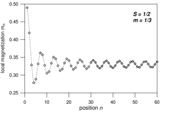
Figure 2: Magnetization profiles determined by the DMRG for the $S=1/2$ chain with $N=120$, $M=160$ and magnetization $m=S^{z}_{\rm tot}/N\approx 1/3$. Only half of the chain shown - the other half is mirror symmetric.

It is worth discussing the fitting procedure itself in some detail. The Ansatz in Eq. (5) has five parameters: $m,A_{m},k_{F},\delta N$ and $\eta_{z}$. Although $S^{z}_{\rm tot}$ is a conserved quantity, and thus can be set to a given value in the DMRG, due to the open boundary condition the control over the exact (bulk) value of $m$ is lost. While it is true that for long enough chains $m$ will be close to $S^{z}_{\rm tot}/N$, the finite size deviation should be tracked during the fitting procedure. Similarly, although $k_{F}$ is a well-specified function of $m$ in the bulk [see Eq. (2)], it was found advantageous to keep it as an independent fit parameter, and only use Eq. (2) a posteriori as a consistency check. On the other hand, it is better to avoid fitting on $\delta N$ directly. Instead the best working alternative seems to be making a four-parameter fit on $m,A_{m},k_{F}$ and $\eta_{z}$, while $\delta N$ kept fixed. The optimal value of $\delta N$ is the one which yields the highest stability with respect to local fits, i.e., calculating the four fitting parameters from a small number of sites at different locations in the chain. An example of this procedure is shown in Fig. 3. We found that the optimal value of $\delta N$ is a weak function of $m$, being about $\delta N\approx 0.5$ for $m=0$, and decreasing monotonically to $\delta N\approx 0.4$ for $m=1/2$. This is more or less consistent with the value $\delta N=1/2$ used in the bosonization approach of Ref. Hik-Fur, .

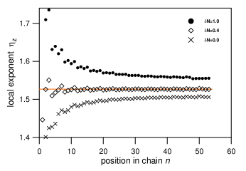
Figure 3: Stability of local fit parameters as a function of local position in the chain for $S=1/2$, $L=120$, $m\approx 1/4$. Local fit parameters at position $n$ are defined by fitting for sites $i=n,\dots,n+3\lambda$, with $\lambda=2\pi/k_{F}=1/(S-m)$ the wavelength of the oscillations. The highest stability of the parameters is achieved for $\delta N\approx 0.4$. Equation (2) is satisfied up to $2.10^{-4}$.

Having obtained $\eta_{z}$ using the above fitting procedure, the fundamental quantity of the theory, the dressed charge $Z$, can be calculated from Eq. (10). Figure 1 shows the numerically determined dressed charge as a function of $m$. The relative error of the fitting procedure is under $0.1\%$, except for very small $m$ values where logarithmic corrections to the fitting formula and $Z$ are expected, and the fitting procedure loses stability (see the error bar in the figure at $m=0.03$). Otherwise, the agreement with the exact values is very good and stable for $0.03\lesssim m<1/2$. For comparison Fig. 1 also shows the estimate of $Z$ when the naive scattering length $\delta N=0$ is used. Even with this the error is within $1\%$, except for very small $m$.

We conclude that for $S=1/2$ the LL Ansatz for the magnetization profile, Eq. (5), is a very efficient tool in calculating the critical exponents (dressed charge). The final result is highly accurate already with $\delta N=0$, but an additional increase in precision can be achieved by adding the scattering length as an extra fit parameter.

IV The $S=1$ chain

Encouraged by the success of the fitting procedure for $S=1/2$, in this section we apply it to the $S=1$ Heisenberg chain. The forthcoming analysis is not intended to prove that the $S=1$ chain in its magnetized regime is a Luttinger liquid - this has been done convincingly already.Tsvelik ; Chi-Gia ; Kon-Fen ; Sak-Tak ; Campos-Venuti Instead, our starting point is the assumption that we have a one-component Luttinger liquid, and then use LL theory and the numerically calculated magnetization profiles to determine the value of $Z$ and the critical exponents with high accuracy.

Although the spin-1 problem cannot be treated rigorously, there are two limits where clear theoretical predictions exist. In the high magnetization limit near saturation the physics can be understood by regarding the system as a dilute gas of magnons created in the ferromagnetic vacuum.Sak-Tak Magnons behave as bosons with short-range repulsive interaction. In the dilute limit the exact form of the interaction is irrelevant and an essentially hard-core boson description becomes valid. In 1D hard-core bosons are equivalent to free spinless fermions, which imply an LL parameter $Z=1$ with correlation exponents $\eta_{z}=2$ and $\eta_{x}=1/2$ as $m\to 1$.

There is a similar argument in the $m\to 0$ limit. Below the critical magnetic field $h_{c}<\Delta_{g}$, where $\Delta_{g}$ is the Haldane gap, the elementary excitations are massive spin-1 bosons.Aff-Sor At $h_{c}$ these bosons condensate, but due to the interboson repulsion the magnetization only increases gradually. Near $m\gtrsim 0$ the boson density is low and by the above argument we again obtain $Z=1$, $\eta_{z}=2$ and $\eta_{x}=1/2$. Note that this argument only works for $S=1$ with a Haldane gap. For $S=1/2$ for which the nonmagnetized ground state is massless, the elementary excitations form a strongly interacting dense gas with $Z=1/\sqrt{2}$ as is given by the Bethe Ansatz, and the SU(2) symmetry at $m=0$. Alternative theories for $S=1$, based on either a Majorana fermion representationTsvelik or on the bosonization of spin-1/2 laddersChi-Gia lead to a similar conclusion in this limit.

Although the magnetized $S=1$ chain is a Luttinger liquid, this classification only applies at low energies and long distances. Indeed, at higher energies and shorter distances the $S=1$ chain produces features which cannot be understood within the framework of LL theory. These features, absent in $S=1/2$ chains, stem from the additional degrees of freedom staying massive for $S>1/2$. These degrees of freedom have signature both in the energy spectrum and correlations, and manifest themselves in the numerical, finite chain calculations. Their origin can be easily understood in the low-magnetization limit. At zero magnetic field the system possesses an energy gap, the Haldane gap. The lowest excited states form a triplet branch with a minimum energy at momentum $k=\pi$. The operator $S_{i}^{z}$ has large matrix elements between the ground state and the $S^{z}_{\rm tot}=0$ component of this triplet. This leads to an exponentially decaying alternating (antiferromagnetic) behavior in the longitudinal correlation function. When the magnetic field is switched on, the Zeeman energy splits the triplet branch, and at $h=\Delta_{g}$ the $S^{z}_{\rm tot}=1$ component at $k=\pi$ crosses over with the ground state. However the $S^{z}_{\rm tot}=0$ component remains in the spectrum (at energy $\approx\Delta_{g}$) and still contributes to the short-range longitudinal correlation functions. As a consequence the two-point function shows a crossover from a seemingly exponential decay on short distances caused by the massive mode to an algebraic decay determined by the soft, LL mode on longer distances.

There is a similar effect in the one-point function we consider here. Near the chain’s end there is an exponentially localized effective $S=1/2$ degree of freedom, the so-called ”end spin”, which also survives in the magnetized regime, at least when the magnetization is not too high.Yam-Miy Its presence produces a crossover from exponential decay to algebraic decay in the one-point correlation function as is illustrated in Fig. 4. As the magnetization increases the massive modes rise in energy, and have a less and less significant impact on the low-energy physics. At the same time the end spins gradually dissolve and disappear in the bulk as was observed by Yamamoto and Miyashita.Yam-Miy

Figure 4: Magnetization profiles determined by the DMRG for the $S=1$ chain with $N=120$, $M=160$ at the bulk magnetization $m\approx 0.097$. Only half of the chain shown - the other half is mirror symmetric. The LL oscillation is clearly visible above $n>20$. Solid line is the LL fit. Inset shows the end of the chain on a log-lin scale featuring the exponentially decaying initial oscillation which crosses over to LL behavior at $n\approx 12$.

In order to measure the critical exponent $\eta_{z}$ we used the DMRG algorithm with $N=120$ and $M=160$ with five iteration cycles. The truncation error varied in the range $1-P_{m}=10^{-12}-10^{-8}$, the calculation being more precise in the high magnetization regime. A limited number of runs with $N=240$, $M=300$ was done to check the numerical precision and to obtain results at points where longer systems were needed. We applied the fitting procedure described above and care was taken to stay in the bulk of the chain sufficiently far from the ends. Since for $m=0$ the correlation (localization) length of the end spin is about 6 lattice sites, which becomes even shorter for $m>0$, a chain length $N=120$ was found sufficient.

We observed that the fitting procedure is somewhat less accurate here than for $S=1/2$, meaning that finite size corrections to the Luttinger liquid profile Eq. (5) are more important in for $S=1$. The fitting procedure becomes especially unreliable below $m\approx 0.05$ and around $m\approx 0.5$. In the former case the increasing wavelength, which becomes comparable to the system size, whereas in the latter case the vanishing prefactor $\cos[2k_{F}(n-(N+1)/2)]\to 0$ can be blamed for the numerical difficulty. Far enough from these problematic regions the relative error of the calculated exponent was estimated to be less than $1\%$.

Beyond measuring the local magnetization profile $m_{n}$, for $S=1$ there is another, independent quantity whose profile can also be measured easily. This is the local quadrupole moment $q_{n}=\langle(S^{z}_{n})^{2}\rangle$. Note that for $S=1/2$ this quantity is redundant and thus carries no additional information. For $S=1$, however, the quadrupole profile provides us an alternative way to measure the critical exponent which in many cases became even more precise than the one obtained through the magnetization profile. The quadrupole profile is expected to behave according to the same scaling form Eq. (5) with the replacement $m\to q$, $A_{m}\to A_{q}$.

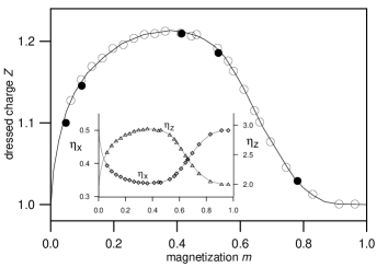
Figure 5: Dressed charge $Z$ determined numerically for the $S=1$ chain. Open symbols denote results for $L=120$, closed symbols for $L=240$. The estimated error is comparable to the symbol size. Solid line is only a guide to the eye. Inset shows the longitudinal and transverse critical exponents $\eta_{z}$ and $\eta_{x}$, resp.

Figure 5 shows the dressed charge determined using Eq. (10) from the measured $\eta_{z}$ exponent of magnetization and quadrupole profiles. The inset also shows the corresponding critical exponents $\eta_{z}$ and $\eta_{x}$ as a function of the bulk magnetization. We see that for $m\to 1$ the predicted value $Z=1$ is reached very rapidly. We analyzed the $m$-dependence close to $m=1$ and found it to be describable with a power law with a rather large exponent around 4, although a scaling faster than any power law cannot be excluded either. Due to the lack of sufficient numerical precision near $m=1$ we were unable to resolve this question reliably.

For $m\to 0$ the conclusion is also somewhat vague because the $m$-dependence is very steep and due to numerical difficulties we were unable to approach this limit closely enough. However, a $Z=1$ value predicted by the theory seems highly consistent with our data. Assuming this, our numerical values seem to indicate an $m$-dependence $Z-1\sim m^{\alpha}$, with $\alpha=0.5\pm 0.1$. Knowing that $m$ scales above the gap as $m\sim\sqrt{h-\Delta_{g}}$,Sak-Tak-98 this would imply $Z-1\sim(h-\Delta_{g})^{\beta}$ for small $h$ with $\beta\approx 1/4$.

Between the two limits $Z$ is larger, reaching its largest value $Z\approx 1.21$ at $m\approx 0.36$. This behavior should be compared to that of $S=1/2$, where $Z<1$ in the whole regime (see Fig. 1). Earlier data on the critical exponents available in the literature, which were determined by other methods such as the finite-size scaling analysis of the energy spectrumSak-Tak ; Usa-Sug or the staggered structure factor,Campos-Venuti are consistent with our results.

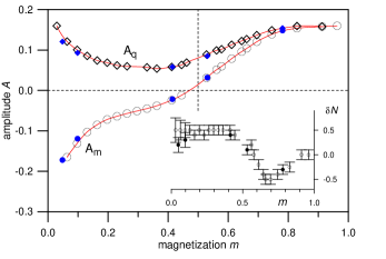
Figure 6: Magnetization and quadrupole moment amplitudes for the $S=1$ chain. Open symbols denote results for $L=120$, closed symbols for $L=240$. Inset shows the best estimate of $\delta N$.

The numerically determined critical amplitudes are depicted in Fig. 6. The amplitude of the magnetic moment fluctuations $A_{m}$ increases monotonically as a function of $m$. However, the rate of increase is not smooth as it is seen in the figure. $A_{m}$ changes sign somewhere close to $m=1/2$. Where $A_{m}\approx 0$ the observable fluctuations are governed by the next smallest critical exponent, and thus a precise measurement is beyond our method. In contrast with this, the amplitude of the quadrupole fluctuations $A_{q}$ remains positive in the whole magnetized regime. We observe that it decreases for small $m$, reaching its minimal (still positive) value at $m\approx 0.36$. Above this it increases and saturates for $m\to 1$.

Finally, it is interesting to note that the optimal value of the scattering length $\delta N$ changes considerably as $m$ varies. As the inset of Fig. 6 shows that $\delta N$ is around $0.5$ for small $m$, then decreasing to $\delta N\approx-0.5$ at $m\approx 0.7$, then increasing again to $\delta N\approx 0$ at $m=1$. There is a relatively large uncertainty in the optimal value determined, but this imprecision has little impact on the estimated value of $Z$ and the correlation exponents.

V Summary

In this paper we have analyzed the critical fluctuations in open $S=1/2$ and $S=1$ Heisenberg chains in their magnetized regime. The low energy physics is a one-component Luttinger liquid in both cases. We have calculated the LL’s characteristic dressed charge and the amplitude of the leading critical fluctuations. Our method consisted of determining numerically the magnetization and quadrupole operator profiles and applying a fitting procedure based on conformal invariance. The method has been thoroughly tested on the Bethe Ansatz solvable $S=1/2$ chain, confirming its reliability and high precision. In the $S=1$ case, where the exact solution is unknown the method provided high-precision estimates of the critical exponents, justifying and complementing earlier results derived by alternative methods. We also determined critical amplitudes which has much less been studied so far for these systems.

Beyond calculating the characteristic parameters with high accuracy our results also allow us to make a detailed comparison between the $S=1/2$ and $S=1$ chains. Although both are Luttinger liquids, the respective dressed charges as functions of the magnetization differ quite considerably. The only limit where the two systems become equivalent is the full saturation limit, $m\to S$, where $Z\to 1$. Otherwise, for $S=1/2$ the dressed charge is $Z<1$, while for $S=1$ it is $Z>1$. There are interesting differences in the behavior of the critical amplitudes and the scattering lengths at the chain ends, as well.

We thank F. Iglói and J. Sólyom for valuable discussions. This work was partially supported by the Hungarian Scientific Research Found (OTKA) under grant Nos. T30173, T43330 and F31949, and by the Bolyai Research Scholarship Program. The numerical calculations were done at the NIIF Supercomputing Facility.

References

- (1) F. D. M. Haldane, Phys. Rev. Lett. 50, 1153 (1983); Phys. Lett. 93A, 464 (1983).
- (2) F. D. M. Haldane, J. Phys. C: Solid State Phys. 14, 2585 (1981).
- (3) F. D. M. Haldane, Phys. Rev. Lett. 45, 1358 (1980).
- (4) A. M. Tsvelik, Phys. Rev. B 42, 10499 (1990).
- (5) R. Chitra and T. Giamarchi, Phys. Rev. B 55, 5816 (1997).
- (6) R. M. Konik and P. Fendley, Phys. Rev. 66, 144416 (2002).
- (7) M. Takahashi and T. Sakai, J. Phys. Soc. Jap. 60, 760 (1991); T. Sakai and M. Takahashi, ibid. 60, 3615 (1991).
- (8) M. Usami and S. I. Suga, Phys. Rev. B 58, 14401 (1998).
- (9) T. Hikihara and A. Furusaki, Phys. Rev. B 63, 134438 (2001).
- (10) M. Oshikawa, M. Yamanaka, and I. Affleck, Phys. Rev. Lett. 78, 1984 (1997).
- (11) G. Fáth and P. B. Littlewood, Phys. Rev. B 58, R14709 (1998).
- (12) A. Gogolin, A. A. Nersesyan, and A. M. Tsvelik, Bosonization and Strongly Correlated Systems, Cambridge University Press, Cambridge (1998).
- (13) F. D. M. Haldane, Phys. Rev. Lett. 47, 1840 (1981).
- (14) L. Campos Venuti, E. Ercolessi, G. Morandi, P. Pieri, M. Roncaglia, Int. J. Mod. Phys. B16, 1363 (2002).
- (15) T. W. Burkhardt and E. Eisenriegler, J. Phys. A: Math. Gen. 18, L83 (1985).
- (16) N. Shibata, K. Ueda, T. Nishino and C. Ishii, Phys. Rev. B 54, 13495 (1996).
- (17) G. Bedurftig, B. Brendel, H. Frahm, and R. M. Noack, Phys. Rev. B 58, 10225 (1998).
- (18) S. R. White, I. Affleck, and D. J. Scalapino, Phys. Rev. B 65, 165122 (2002).
- (19) M. E. Fisher and P. G. de Gennes, C. R. Acad. Sci. Paris B 287, 207 (1978).
- (20) R. B. Griffiths, Phys. Rev. 133, A768 (1964); C. N. Yang and C. P. Yang, ibid. 133, 321 (1966); ibid. 133, 327 (1966).
- (21) J. L. Cardy in Phase Transitions and Critical Phenomena ed. by C. Domb and J. L. Lebowitz (Academic, New York, 1987) vol. 11.
- (22) F. Woynarovich and H.-.P Eckle, J. Phys. A20, L97 (1987); H. J. de Vega, Int. J. Mod. Phys. A 4, 2371 (1989).
- (23) J. B. Parkinson, J. Phys.: Condens Matter 1, 6709 (1989); A. Schmitt, ”Exakt lösbare Spin-1 Modelle”, PhD thesis, University of Wuppertal (1996); D. C. Cabra, A. Honecker and P. Pujol, Phys. Rev. B 58, 6241 (1998).
- (24) S. R. White, Phys. Rev. Lett. 69, 2863 (1992); S. R. White, Phys. Rev B 48, 10345 (1993).
- (25) I. Affleck, Phys. Rev. B 43, 3215 (1991); E. S. Sorensen and I. Affleck, Phys. Rev. Lett. 71, 1633 (1993).
- (26) S. Yamamoto and S. Miyashita, Phys. Rev. B 51, 3649 (1995).
- (27) T. Sakai and M. Takahashi, Phys. Rev. B 57, R8091 (1998).