Spectral densities of Kondo impurities in nanoscopic systems

Abstract

We present results for the spectral properties of Kondo impurities in nanoscopic systems. Using Wilson’s renormalization group we analyze the frequency and temperature dependence of the impurity spectral density $\rho_{i}(\omega,T)$ for impurities in small systems that are either isolated or in contact with a reservoir. We have performed a detailed analysis of the structure of $\rho_{i}(\omega,T)$ for $\omega$ around the Fermi energy for different Fermi energies relative to the intrinsic structure of the local density of states. We show how the electron confinement energy scales introduce new features in the frequency and temperature dependence of the impurity spectral properties.

I Introduction

The physics at the nanoscale has emerged as one of the most active areas in condensed matter physics. This new field includes the study of small metallic and superconducting islands, quantum dots and nanostructurated semiconductors, nanotubes and quantum corrals, nanoelectronics and nano-characterization among other things.nanoscience

The advances in nanotechnologies revived the interest in the Kondo effect,Hewson1993 one of the paradigms of strongly correlated systems. On one hand, Scanning Tunneling Microscopy (STM) allowed the direct measurement of local spectroscopic properties of Kondo impurities on noble metal surfacesmadhavan98 ; nagaoka2002 and in nanoscopic systems.Manoharan2000 On the other hand, it has been shown that single electron transistors and single walled carbon nanotubes weakly coupled to contacts may behave as Kondo impurities generating new alternatives to study the phenomena.Meir1991

In its simplest form, the Kondo problem is a single quantum spin interacting with an ideal electron gas. An antiferromagnetic coupling between the impurity and the free electron spins gives rise to an anomalous scattering at the Fermi energy leading to a large impurity contribution to the resistivity. Simultaneously the impurity spin is screened by the conduction electrons and the magnetic susceptibility saturates at low temperature. There is a characteristic temperature $T_{K}$ that separates the low temperature from the high temperature regimes. At $T\gg T_{K}$, the impurity spin is essentially free and the problem can be treated by perturbations in a dimensionless coupling constant $\lambda$. At $T\ll T_{K}$ the impurity spin is screened forming a singlet complex with the conduction electrons and the system is described by an infinite effective coupling. The crossover regime with $T\sim T_{K}$ is more difficult to describe and the best treatment corresponds to the numerical renormalization group (NRG) as done by Wilson.Wilson1975

The characteristic Kondo temperature is given by $T_{K}$ $\sim D\sqrt{\lambda}e^{-1/\lambda}$ where $2D$ is the free electron bandwidth. Associated to this energy scale there is a characteristic length scale known as the Kondo screening length $\xi_{K}=\hbar v_{F}/$ $k_{B}T_{K}$ where $v_{F}$ is the Fermi velocity. The physical meaning of the screening length is that, in the low temperature regime where the impurity spin is screened, the antiferromagnetic correlations between the impurity and conduction electron spins extend up to a distance of the order of $\xi_{K}$.

The problem of Kondo impurities in nanoscopic systems for different experimental realizations has been the subject of many recent theoretical and experimental works.Thimm1999 When a Kondo system, either an atomic impurity or an artificial atom like a quantum dot (QD), is embedded in a small system of volume $L^{d}$ where $d$ is the spacial dimension, the length-scale $L$ should be compared with the characteristic Kondo length $\xi_{K}$. For $L<\xi_{K}$ finite-size effects are expected to be important. The condition $L\sim\xi_{K}$ is equivalent to $k_{B}T_{K}\sim\Delta$ where the energy $\Delta$ gives the average level spacing of the finite system. For a finite system the characteristic energy $\Delta$ acts as a low energy cutoff for the charge and spin excitations and consequently it modifies the low temperature behavior of the system.

The ground state properties of a Kondo impurity in a small system have been addressed by a number of authors using different approximations.Thimm1999 ; Cornaglia2002 ; Affleck2001 The thermodynamic properties and the effect of coupling the system to a macroscopic reservoir have recently been studied using the Wilson’s renormalization group.Cornaglia2002 In this work we extend renormalization group calculations to evaluate the impurity spectral density and analyze how the new energy or length scales introduced by the finite size affects the Kondo resonance at the Fermi energy. We also study the temperature dependence of the low energy spectral density.

The rest of the paper is organized as follows: in section II we present the model and describe how the numerical renormalization group is adapted to our case. We then recap the most relevant thermodynamic properties. Section III contains the spectral properties of the impurity for frequencies close to the Fermi energy. After presenting the general formulation we show results for finite systems, systems in contact with a reservoir and the temperature dependence of the Kondo resonances. Finally section IV includes a summary and discussion.

II Model and Thermodynamic properties

In this section we present the model for an impurity in a nanoscopic system coupled with a macroscopic reservoir and briefly discuss how Wilson’s renormalization group is adapted to this problem. Then we review the thermodynamic properties of the system.

II.1 Model Hamiltonian and Wilson’s Renormalization Group

Our starting point is the Anderson model for magnetic impurities with a Hamiltonian which in the usual notation reads:Anderson1961

$$H_{AM} = \sum_{\sigma}\varepsilon_{d}d_{\sigma}^{\dagger}d_{\sigma}+Ud_{\uparrow}^{\dagger}d_{\uparrow}d_{\downarrow}^{\dagger}d_{\downarrow}+\sum_{\nu,\sigma}\varepsilon_{\nu}c_{\nu\sigma}^{\dagger}c_{\nu\sigma}$$ (1)

$$+\sum_{\nu,\sigma}(V_{\nu}^{*}c_{\nu\sigma}^{\dagger}d_{\sigma}+V_{\nu}d_{\sigma}^{\dagger}c_{\nu\sigma})-\mu_{i}BS_{iz},$$

where the operator $d_{\sigma}^{\dagger}$ creates an electron with spin $\sigma$ at the impurity orbital with energy $\varepsilon_{d}$ and Coulomb repulsion $U$, and $c_{\nu\sigma}^{\dagger}$ creates an electron in an extended state with quantum numbers $\nu$ and $\sigma$ and energy $\varepsilon_{\nu}$. The last term represents the effect of an external magnetic field along the $z$-direction coupled to the impurity spin ${\bf S}_{i}$. Hereafter we will use $D=1$ as our unit of energy.

In this notation, the nanostructure of the system is hidden in the structure of the one-electron extended states with energies $\varepsilon_{\nu}$ and wavefunctions $\psi_{\nu}({\bf r})$. In equation (1) the hybridization matrix elements are taken proportional to the extended state wavefunctions at the impurity position, i.e. $V_{\nu}=V_{0}\psi_{\nu}(0)$ where the impurity position is defined as the origin of coordinates. We consider a simple structure consisting of a spherical metallic cluster of radius $R_{c}$ with the impurity at the center. The cluster is embedded in a bulk material with which it is weakly coupled through a large surface barrier. The Hamiltonian can be put in the form $H_{AM}=H_{AM}^{0}+W(r,R_{c})$ where the first term is the Anderson model Hamiltonian for an impurity in an infinite homogeneous host and the last term is a spherically symmetric potential barrier placed at a distance $R_{c}$ from the impurity. Figure 1(a) illustrates the configuration described by the model. For an infinite impenetrable barrier, the central cluster is decoupled from the macroscopic reservoir and the model describes an impurity in a small sample. In this situation, the extended states that are coupled to the impurity, are confined in the central cluster and their energy spectrum is a discrete spectrum with a mean energy level separation given by the characteristic energy $\Delta.$ For a finite barrier these states are hybridized with the continuum acquiring a finite lifetime, the local density of states inside the central cluster then presents resonances separated by the energy $\Delta$ and with widths $\gamma$ that are determined by the barrier. The model then incorporates the new energy scales $\Delta$ and $\gamma$, that may drastically change the impurity behavior.

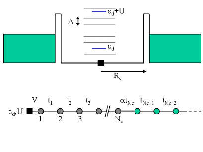
Figure 1: A sketch of the central grain embedded in a metal (a). Inside the grain the characteristic energy level spacing $\Delta$ is shown together with the impurity levels at $\varepsilon_{d}$ and $\varepsilon_{d}+U$. In (b) the linear chain obtained after Wilson’s canonical transformation.

This geometrical structure is particularly appropriate to use the numerical renormalization group approach developed by Wilson. Wilson introduced a logarithmic discretization of the energy of the conduction electrons, dividing the band in a series of energy intervals with exponentially decreasing width. By means of a canonical transformation the resulting Hamiltonian can be mapped into a linear chain with variable hoppings. Each site representing an orbital surrounding the impurity with an associated energy (or length) scale. Wilson proposed to solve the linear chain by iterative perturbation. A truncated chain with $N$ sites, described by an effective Hamiltonian $H_{N}$, gives the correct physics on an energy scale $\tilde{\omega}_{N}$. A renormalization group transformation corresponds to adding a site to the chain and relates the Hamiltonians describing successive lower energy scales. This leads to a systematic way of calculating the thermodynamic properties at successive lower temperatures and the spectroscopic properties at successive lower frequencies.

In our case, the Hamiltonian $H_{AM}^{0}$ is rewritten in Wilson’s basis as schematically shown in Fig.1(b). The potential barrier is described including a higher diagonal energy to the orbital centered around $R_{c}$. Due to the structure of Wilson’s basis wavefunctions, a given potential barrier leads to a diagonal energy that decreases as $R_{c}$ increases. Alternatively the barrier can be simulated with a smaller hopping matrix element in the region where $W(r,R_{c})$ is different from zero. We adopted this last description reducing one hopping term by a factor $\alpha$. In what follows it is assumed that the band of extended states is half filled - the Fermi energy is set equal to zero - and $\epsilon_{d}=-U/2$. This guarantees that the electron-hole symmetry of the problem is preserved.

The properties of a Kondo impurity depend on the local density of states at the impurity coordinate that in Wilson’s representation is the local density of states at site 1. We end this section with a brief discussion on the effect of the confining potential $W(r,R_{c})$ on the local density of states close to the Fermi energy. For a given $N$ the spectrum of $H_{N}$ depends on the parity of $N$. In the absence of impurity, a one particle state at zero energy exists only for odd $N$ as schematically shown in Fig. 2. The spectrum, as a function of $N$, alternates between those of Figs. 2(a) and 2(b). The mean energy separation, between the one-electron states, is given by the characteristic energy $\Delta$ that decreases as $N$ increases. This is the spectrum of a finite system ($N=N_{c}$) described by an infinite barrier. The other one electron states, not shown in Fig. 2, are not at energies $n\Delta$ or $(n+1/2)\Delta$ with integer $n$. This is due to the logarithmic discretization of the band. How the NRG can be used to analyze finite size effects was shown by NozieresNozieres . To show that the logarithmic discretization correctly describes the low energy spectrum of a impurity in finite systems, in the next section, we compare the exacts results on a finite system with those obtained with the NRG. The alternating spectrum with a fixed Fermi energy corresponds to an alternating parity in the number of electrons, in fact for a fixed electron density, as the radius $R_{c}$ of the cluster increases, the number of electrons alternates between even and odd. We recall that due to the symmetry of the system only the sector of the Hilbert space with s-wave electrons is considered here.

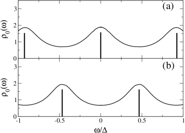
Figure 2: Unperturbed local density of extended states at the impurity coordinate (site 1) for a cluster with $\alpha=0$ (vertical bars) and $\alpha=0.05$ (lines). In the later case the spectral density has been evaluated using a small imaginary part in the frequency (a) $N_{c}=19$ and (b) $N_{c}=20$.

With a finite barrier ($\alpha\neq 0$) the discrete states of the cluster are hybridized with the continuum of the host metal and become resonances. The local density of states then becomes a continuum but retains some structure characterized by the energy $\Delta$. In the NRG approach, Hamiltonians $H_{N}$ with $N>N_{c}$ accumulate states at low energies representing the broadening of the central peak for odd $N_{c}$ or the tails of the states at $\pm\Delta/2$ for even $N_{c}$. The local densities of states as obtained with the NRG are also shown in Fig. 2. For $\alpha\neq 0$ the number of electrons in the central cluster is no longer a good quantum number and in what follow we refer to the situations of Figs. 2(a) and 2(b) as the Fermi energy being at a resonance (at-resonance) or between two resonances (off-resonance) respectively.

As we show below, this structure of the local density of states determines the thermodynamic and the spectral properties of the impurity.

II.2 Thermodynamic Properties

Here we briefly recap the thermodynamic properties of the model. As stated above, for $\alpha=0$ the at-resonance situation corresponds to an odd number of extended electrons. An impurity in the Kondo limit contributes with an extra electron and the ground state is a singlet indicated as $|0\rangle.$ The expectation value of the impurity spin $\langle 0|S_{iz}|0\rangle$ is zero reflecting the complete screening of the impurity spin and the zero temperature susceptibility is finite. For the off-resonance situation the ground state of the isolated cluster with a Kondo impurity is a Kramers spin-$1/2$ doublet, $|\Uparrow\rangle$ and $|\Downarrow\rangle$. The expectation value $\langle\Uparrow|S_{iz}|\Uparrow\rangle=-\langle\Downarrow|S_{iz}|\Downarrow\rangle$ is different from zero and, in the low temperature limit the impurity susceptibility diverges as $\chi=\mu_{i}^{2}\langle\Uparrow|S_{iz}|\Uparrow\rangle^{2}/k_{B}T$.

For a finite barrier the susceptibility always saturates, however the at-resonance and off-resonance situations give rise to very different temperature dependences. We calculated the impurity magnetic susceptibility given by Desc

$$k_{B}T\chi = {\mu}_{i}^{2}(\sum_{\nu}P_{\nu}|\langle\nu|S_{iz}|\nu\rangle|^{2}+$$ (2)

$$2k_{B}T\sum_{\nu\neq\xi}|\langle\nu|S_{iz}|\xi\rangle|^{2}\frac{P_{\nu}}{E_{\xi}-E_{\nu}}),$$

where the summation is done over the low energy states $|\nu\rangle$ with energies $E_{\nu}$ and $P_{\nu}=\exp(-E_{\nu}/k_{B}T)/Z$. The matrix elements $\langle\nu|S_{iz}|\xi\rangle$ have to be evaluated in a recursive way at each renormalization step. The susceptibility reflects the thermodynamic properties of the system and we use the effective magnetic moment ${\mu}^{2}=k_{B}T\chi$ as an indicator of the degree of screening of the impurity spin.

In absence of barrier - corresponding to the infinite homogeneous system - the characteristic energy scale is the Kondo temperature indicated as $k_{B}T_{K}^{\infty}$. A finite barrier at $R_{c}$ - enclosing $N_{c}$ shells- introduces the new energy scale $\Delta\cong D\Lambda^{-N_{c}/2}$, where $\Lambda=2$ is Wilson’s discretization parameter. For $k_{B}T_{K}^{\infty}\gg\Delta$ the fine structure (on the scale of $T_{K}^{\infty}$) of the density of states does not change the properties of the system. Conversely, for $k_{B}T_{K}^{\infty}\sim\Delta$ new confinement induced regimes are observed: for the system at-resonance, as the temperature is lowered, there is a rapid decrease in the magnetic moment ${\mu}^{2}$ when $k_{B}T\sim\Delta$; for the system off-resonance, as $k_{B}T$ approaches $\Delta$ the magnetic moment saturates leading to a plateau in the temperature dependence of ${\mu}^{2}$, only at lower temperatures the screening is completed (see Fig. 3). This plateau can be interpreted as the behavior of an isolated cluster. Only at very low temperatures the coupling with the host states becomes relevant and the complete screening can occur. The condition for the existence of these new regimes $k_{B}T_{K}^{\infty}\sim\Delta$ can be put in the form $\xi_{K}^{\infty}$ $\sim R_{c}$ where $\xi_{K}^{\infty}=\hbar v_{F}/k_{B}T_{K}^{\infty}$ is the Kondo screening length of the infinite system. In other words, only if the Kondo screening length is of the order or larger than the system size, the confinement effects become evident in the thermodynamic properties.

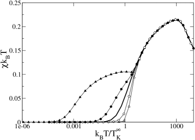
Figure 3: The magnetic susceptibility $k_{B}T\chi$ versus temperature. The thick line corresponds to an impurity in a bulk material ($\alpha=1$), lines and symbols to a barrier enclosing $N_{c}=19$ and $20$ shells (open and full symbols respectively). Triangles (circles) correspond to $\alpha=0.35$ $(0.6)$. The other parameters are: $\varepsilon_{d}=-0.5$, $U=1.0$, and $V=0.2$.

Although the behavior of the system is not universal, at very low temperatures the susceptibility can be used to define an effective Kondo temperature. In fact the low temperature tail of $k_{B}T\chi$ can be scaled to define the effective energy scale $T_{K}^{eff}$ for the low energy spin excitations. We have done this using two different criteria, one is simply to use Wilson’s result:

$$\chi(T=0)=0.103\frac{{\mu}_{i}^{2}}{k_{B}T_{K}},$$ (3)

to relate the low temperature susceptibility to an effective $T_{K}^{eff}$. The other alternative is to plot ${\mu}^{2}$ vs. $T/T_{K}^{eff}$ fitting $T_{K}^{eff}$ to have a good scaling at low temperatures. The effective Kondo temperatures describing the low temperature behavior are shown in Fig. 4 as a function of the barrier height for the at-resonance and off-resonance situations. For $\alpha>0.2$ the two criteria give the same results, for smaller values of $\alpha$ the universal behavior is obtained only at extremely low temperatures where numerical errors become important.

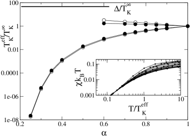
Figure 4: The effective Kondo temperature, that describes the low temperature behavior of the susceptibility, versus the barrier parameter $\alpha$ for the at-resonance (upper curves) and the off-resonance (lower curves) cases. Open symbols were obtained using Eq. (3), full symbols using the scaling shown in the inset. The parameters are the same as in Fig. 3.

III Spectral Densities of Impurities in Nanoscopic Systems

Using the standard definitions and notation, the impurity Green’s function can be written, using the Lehmann representation, as:

$$G_{\sigma}(\omega,T)=\frac{1}{Z(T)}\sum_{\lambda,\lambda^{\prime}}|\langle\lambda|d_{\sigma}|\lambda^{\prime}\rangle|^{2}\frac{e^{-E_{\lambda}/k_{B}T}+e^{-E_{\lambda^{\prime}}/k_{B}T}}{\omega-(E_{\lambda^{\prime}}-E_{\lambda})},$$ (4)

where $Z(T)$ is the grand partition function

$$Z(T)=\sum_{\lambda}e^{-E_{\lambda}/k_{B}T}.$$ (5)

The corresponding impurity spectral density is

$$\rho_{i\sigma}(\omega,T) = -\frac{1}{\pi}[G_{\sigma}(\omega+i0^{+},T)-G_{\sigma}(\omega-i0^{+},T)]$$ (6)

$$= \frac{1}{Z(T)}\sum_{\lambda,\lambda^{\prime}}|M_{\lambda,\lambda^{\prime}}|^{2}(e^{-E_{\lambda}/k_{B}T}+e^{-E_{\lambda^{\prime}}/k_{B}T})\times$$

$$\delta(\omega-(E_{\lambda^{\prime}}-E_{\lambda})),$$

with $M_{\lambda,\lambda^{\prime}}=\langle\lambda|d_{\sigma}|\lambda^{\prime}\rangle$. In the absence of an external magnetic field, the impurity spectral density is spin independent and from here on we drop the spin index in $\rho_{i\sigma}(\omega,T)$.

We now briefly discuss the application of the NRG to evaluate these quantities. The zero temperature limit of expression (6) can be put in the form:

$$\rho_{i}(\omega,T=0) = \frac{1}{Z(0)}\sum_{\lambda,0}|M_{\lambda,0}|^{2}\delta(\omega+E_{\lambda})$$ (7)

$$+|M_{0,\lambda}|^{2}\delta(\omega-E_{\lambda}),$$

where the subindex $0$ indicates the ground state, the summation is over all excitations $\lambda$ with energies $E_{\lambda}$ and on the components of the ground state in the case of a degenerate ground state, $Z(0)$ is the zero temperature partition function that gives the ground state degeneracy. We recall that in the NRG the chemical potential is set at zero and all many body energies $E_{\lambda}$ are measured from the ground state energy.

In order to evaluate the impurity spectral density of the real system using the results of the NRG, consider the spectral density $\rho_{i}^{N}(\omega,T)$ corresponding to Hamiltonian $H_{N}.$ As mentioned above, the RG strategy of an iterative diagonalization of a sequence of Hamiltonians $H_{N}$ with $N=0,1,\ldots$ is based on the fact that, on an energy scale $\tilde{\omega}_{N}$, the spectrum of $H_{N}$ is representative of the spectrum of the infinite Hamiltonian $H$. Hence, for $\omega\approx\tilde{\omega}_{N}$ it is a good approximation to takeHofstetter

$$\rho_{i}(\omega,T=0)=\rho_{i}^{N}(\omega,T=0).$$

A typical choice is to consider for the $N^{th}$ iteration the energy range $\Lambda^{-N/2}<\omega<2\Lambda^{-N/2}$ , that is to consider all the states of $H_{N}$ with energies $E_{\lambda}^{N}$ in this range and all the corresponding matrix elements $M_{\lambda,0}^{N}$ to compute the spectral density as

$$\rho_{i}(\omega,T = 0)=\frac{1}{Z_{N}(0)}\sum_{\lambda,0}|M_{\lambda,0}^{N}|^{2}\delta(\omega+E_{\lambda}^{N})$$ (8)

$$+|M_{0,\lambda}^{N}|^{2}\delta(\omega-E_{\lambda}^{N}).$$

Since for the infinite systems the energy spectrum consists of a continuum, at each energy scale $\tilde{\omega}_{N}$, the discrete spectra are usually smoothed by replacing the delta function $\delta(\omega-E_{\lambda}^{N})$ by a smooth distribution $P_{N}(\omega-E_{\lambda}^{N})$. At each $N$ we use a Gaussian logarithmic distribution with a width that decreases as the characteristic energy scale of $H_{N}$. It is then clear that at high energies, say the atomic energy of the impurity level $\varepsilon_{d}$, the NRG cannot resolve any detailed structure, only at low frequencies there is enough resolution to see, for example, confinement effects. We analyze in detail the impurity spectral density around the Fermi energy which in fact contains all the physics at an energy scale relevant for the Kondo effect and for the electron confinement in a nanoscopic sample.

Before presenting the renormalization group results we show, as a reference calculation, some exact results in finite systems.

III.1 Exact results in finite systems

Here we present the zero temperature results for an impurity in a finite system consisting of a linear chain of $N$ equivalent sites with the impurity at one end. In this case the energy spectrum of extended states $\varepsilon_{\nu}$ and the hybridization matrix elements $V_{\nu}$ of Hamiltonian (1) are given by:

$$\varepsilon_{\nu}=-2t\cos(\nu\pi/(N+1)),$$

and

$$V_{\nu}=V_{0}\sin(\nu\pi/(N+1)),$$

where $t$ is the hopping matrix element in the chain and $\nu=1,2,....,N$.

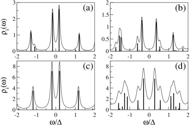
Figure 5: Impurity spectral density $\rho_{i}(\omega,T=0)$. Upper panels are exact results for a linear chain with $N=8$ ($V_{0}=0.14t,\,\epsilon_{d}=E_{F}-0.5t$, $U=1.0t$, and $t=0.25$) and $8$ (a) and $7$ (b) electrons. Lower panels are the NRG results with $\alpha=0$, $N_{c}=13$ (c) and $N_{c}=14$ (d). ($\varepsilon_{d}=-0.5$, $U=1.0$, and $V=0.2$.)

Using a Lanczos algorithm we first calculate the ground state energy and wavevector. In the present case it is convenient to use a second Lanczos algorithmGagliano89 to evaluate directly the impurity spectral function, rather than evaluating excited states, their corresponding energies and matrix elements $M_{\lambda,\lambda^{\prime}}$. For a better comparison of the different cases, we always measure the frequency from the Fermi energy $E_{F}$ defined as $E_{F}=[E_{0}(N_{e}+1)-E_{0}(N_{e}-1)]/2$ with $E_{0}(N_{e})$ the ground state energy of the system with $N_{e}$ particles. The spectral density around the Fermi energy shows a series of peaks separated by the characteristic energy $\Delta$. Each peak may be composed by a one or a few delta lines as shown in Figs. 5(a) and 5(b). In what follows we discuss the low energy structure ($\omega\lesssim\Delta$) of the impurity spectral function for the case of even and odd number of particles corresponding to the at-resonance and off-resonance situations respectively. Note that the results of Figs. 5(a) and 5(b) are not for a half filed system and as a consequence the electron-hole symmetry is not exactly preserved.

Even number of particles: The ground state of the system is a singlet and the impurity spectral density shows a central peak at $\omega\sim 0$ and two satellites at $\omega\sim\pm\Delta$. The central peak consists of two lines, one for $\omega>0$ and one for $\omega<0$ corresponding to adding and subtracting a particle respectively. The splitting between these two lines, that decreases as $V_{0}$ decreases, is not given directly by the confinement energy $\Delta$ but by the energy gained by forming the singlet, i.e. is given by the Kondo temperature of the finite system. The peaks at $\omega\sim\pm\Delta$ are also made of a couple of delta lines each. The justification of this description of a central line and satellites at $\pm\Delta$ is given by the fact that for smaller hybridizations the two central lines approach $\omega\sim 0$ and the impurity spectral density reproduces the structure of the unperturbed local density of states (the at-resonance situation of Fig. 2(a)). Here we used these parameters for a better comparison; results with a smaller hybridization calculated with the NRG are shown below.

Odd number of particles: The ground state of the system is a spin-1/2 doublet. The spectral densities have a low frequency gap with peaks at $\omega\sim\pm\Delta/2$ . Each of these peaks at $\omega\sim\pm\Delta/2$ consist of two delta lines that correspond to final states with different total spin: when an electron is created or destroyed on the spin-1/2 ground state, the final state may have total spin zero or one. The energy of the final state depends on its total spin. Again in this case the general structure is that of the underlying local density of states.

These results should serve us as a guide for the numerical renormalization group calculation. Since the NRG involves some approximations and will be extended to more realistic cases, as is the case of a system with a finite barrier, it is important to have this exact result as a reference calculation.

III.2 Numerical Renormalization Group: Zero Temperature Results

For a finite system, the renormalization procedure is truncated at an iteration $N_{c}$. In Figs. 5(c) and 5(d) we present the NRG results for the impurity spectral density of a finite system with an even and an odd number of particles respectively. As for the calculation of the thermodynamic properties, the system with an even (odd) number of particles is evaluated with an odd (even) number of shells $N_{c}$. The spectrum consists of a discrete collection of delta lines and, as in the previous section, the smoothing is done only for practical purposes in the presentation of the data. Our low frequency NRG results compare very well with the exact results of a finite system [Figs. 5(a) and 5(b)]. Again, for an even number of particles the impurity spectral density consists of a central peak, composed by two delta functions, and the two satellites at $\omega\sim\pm\Delta$. For an odd number of particles the approximate NRG results clearly show the central pseudogap and the two satellites at $\omega\sim\pm\Delta/2$ with a structure that comes from the spin-dependent energy of the final state.

For the remainder, we focus on the more interesting case of a system in contact with a macroscopic reservoir. This is described with a non-zero parameter $\alpha$ representing a finite wall.

In Fig. 6(a) the impurity spectral density for the at-resonance situation is shown for different values of $\alpha$. For $\alpha=0$ the isolated cluster results are reproduced with a peak at low frequencies. This peak is well separated from the Fermi energy due to a large hybridization $V$ used in the calculation for practical purposes. In the figure only a detail of the low frequency structure is shown and the satellite at $\omega\sim\Delta$ is not observed. As $\alpha$ approaches one, corresponding to an infinite homogeneous system, the two structures merge into a single Kondo peak centered at the Fermi energy.

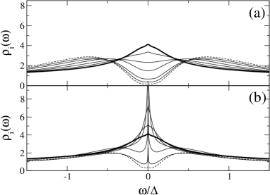
Figure 6: Impurity spectral density $\rho_{i}(\omega,T=0)$ for the at-resonance case with $N_{c}=19$ (a) and the off-resonance case with $N_{c}=20$ (b) and different values of $\alpha$: $\alpha=0.2$ (dashed line), $0.3$, $0.4$ , $0.6$, $0.75$, and $0.9$ (thick line). ($\varepsilon_{d}=-0.5$, $U=1.0$, and $V=0.2$.)

The impurity spectral density when the Fermi energy is off-resonant is shown in Fig. 6(b). For a small $\alpha$ the excitations around $\omega\sim\Delta/2$ are clearly observed. As $\alpha$ increases the $\omega\sim\Delta/2$ structure is washed out and simultaneously a narrow Kondo resonance develops at the Fermi energy.

For more realistic parameters (a smaller hybridization and consequently a smaller Kondo temperature) the at-resonance and off-resonance impurity spectral densities are shown in Fig. 7. These results show that, for the general case of a Kondo impurity in a nanoscopic system with an intermediate barrier and the Fermi energy at a resonant state, we should expect the low frequency spectral density $\rho_{i}(\omega,T=0)$ to present a broad Kondo resonance with some structure. In fact, for large barriers (small $\alpha$), the Kondo resonance has a minimum at the Fermi energy. For the off-resonant case, we expect the spectral density to present the structures at $\omega\sim\pm\Delta/2$ separated by a pseudogap and - at zero temperature - a central Kondo peak.

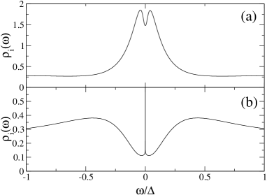
Figure 7: Same as in Fig. 6 with $\alpha=0.45$ and $V=0.15$. a) At-resonance case with $N_{c}=19$ and b) Off-resonance case with $N_{c}=20$.

As we show in the next section, a small temperature completely destroys this central Kondo peak while the broad structures survive up to much higher temperatures.

III.3 Phenomenological approach

Here we briefly discuss the structure of the Kondo resonance in terms of what would be obtained with a simple slave boson theory in the saddle point approximation. In this theory ($U=\infty$), the low energy impurity Green’s function is given by Hewson1993

$$G\left(\omega\right)=\frac{b^{2}}{\omega-\varepsilon_{\lambda}-b^{2}V^{2}g^{0}\left(\omega\right)}$$ (9)

where $b^{2}$ is the square of the mean value of the boson field, $\varepsilon_{\lambda}\simeq 0$ gives the position of the Kondo resonance and $g^{0}(\omega)$ is the bare local propagator of conduction electrons. Here as in the NRG calculation we take the Fermi energy equal to zero. In an homogeneous system it is a good approximation to take $g^{0}(\omega)=-i\pi\rho$ where $\rho$ is the frequency independent local density of states and defining the Kondo temperature $T_{K}$ as the width of the Kondo resonance the local propagator can be put as $G(\omega)\simeq b^{2}/(\omega+iT_{K})$ with $b^{2}=T_{K}/\pi V^{2}\rho$ in agreement with the Friedel’s sum rule. For our case of a central grain weakly coupled with a reservoir, the propagator $g^{0}(\omega)$ is taken as a sum of poles separated by the characteristic energy $\Delta$ and widths $\gamma$

$$g^{0}(\omega)=\sum_{l}\frac{1}{\omega-\Delta_{l}+i\gamma}$$ (10)

with $\Delta_{l}=l\Delta$ or $\Delta_{l}=(l+1/2)\Delta$ for the at-resonance and off-resonance cases respectively. The structure of the Kondo resonance so obtained is shown in Fig 8. The results are in good qualitative agreement with the NRG results. In the at-resonance case, depending on the value of the parameters, the low energy spectrum consists of two peaks with a deep at the Fermi level or a single peak with a maximum at the Fermi level (not shown). In the off-resonance case, a central peak at the Fermi level is obtained. Note however that the area of the central peak relative to the area of the satellite peaks obtained is this approximation is different from that obtained with the NRG.

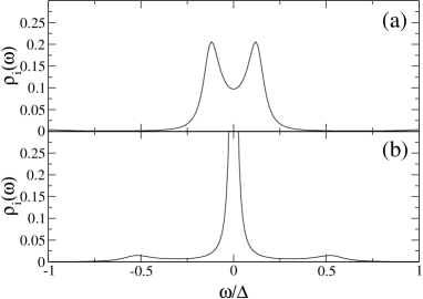
Figure 8: Phenomenological results for the impurity spectral densities. ($\Delta=1.0$, $\gamma=0.1$, and $b^{2}V^{2}=0.02$). a) At-resonance. b) Off-resonance.

III.4 Finite Temperature Results

The NRG calculation of the finite temperature spectral density $\rho_{i}(\omega,T)$ relies on the same approximations of the $T=0$ case. The spectral density at a fixed temperature $T$ is evaluated as above - using Eq. (6) instead of Eq. (7) - if $\omega>k_{B}T$. To calculate the spectral density at $\omega\lesssim k_{B}T$ a Hamiltonian $H_{N}$ with $N$ such that $\tilde{\omega}_{N}\sim k_{B}T$ is used.

When $T_{K}^{\infty}\sim\Delta$ and the Fermi energy lies between resonances, the off-resonance case, two energy scales are clearly observed in the temperature dependence of the susceptibility. In fact as the temperature is lowered they determine the onset of the plateau in $k_{B}T\chi$, that is given by $\Delta$, and the offset at $T_{K}^{eff}$ that is determined by $\alpha$. For the at-resonance case the static magnetic properties are dominated by the larger scale $\Delta$ since for $k_{B}T<\Delta$ the magnetic moment is completely screened. The spectral densities are also sensitive to the temperature and as we will see, there are changes in $\rho_{i}(\omega,T)$ each time the temperature approaches each one of the characteristic energy scales.

In Fig. 9(a) the spectral density $\rho_{i}(\omega,T)$ is shown at different temperatures for a system with the parameters as in Fig. 6. The Kondo peak develops and reaches its zero temperature value as soon as the temperature goes below $\Delta$. The parameters are the same as in Fig. 3 with $\alpha=0.35$.

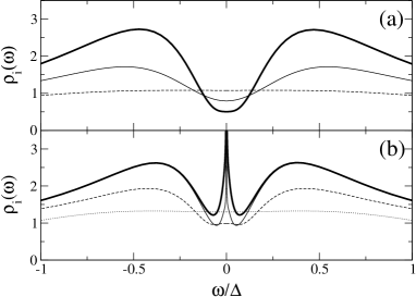
Figure 9: Impurity spectral density $\rho_{i}(\omega,T)$ for different temperatures. (a) At-resonance: $T=0$ (thick line), $T=0.23\Delta$ (thin line), and $T=0.7\Delta$ (dashed line) (b) Off-resonance: $T=0.0$ (thick line), $T=2.0\times 10^{-3}\Delta$ (thin line), $T=5.1\times 10^{-2}\Delta$ (dashed line), and $T=0.5\Delta$ (dotted line).

For the off-resonant situation the temperature evolution is shown in Fig. 9(b). In this last case the two characteristic temperatures are also reflected in the magnetic susceptibility from which we can extract their values as the onset and offset of the plateau in $\mu^{2}$. As can be seen from the figure, as the temperature is lowered, the broad satellite at $\omega\sim\Delta/2$ develops at a temperature corresponding to the onset of the plateau while a narrow Kondo structure develops at a temperature corresponding to the offset of the plateau. The first and second temperatures at which the narrow Kondo peak and the broad structure disappear indicate the decoupling of the impurity spin with the electron spin density at large ($r>R_{c}$) and short ($r<R_{c}$) distances respectively.

IV Summary and Discussion

We have presented a model for a Kondo impurity in a nanoscopic sample or grain coupled with a reservoir through a large barrier. The natural energy - or length - scale associated to the Kondo effect in a bulk material is to be compared with the new scale introduced by the confinement of electrons. These new scales modify the local density of states at the impurity site and consequently their thermodynamic and spectral properties.

The local density of states of the host material consists of resonant states separated by a characteristic energy $\Delta$ and with a width $\gamma$. While $\Delta$ is determined by the size ($R_{c}$) of the grain, the width of the resonances is determined by the transparency ($\alpha$) of the barrier. We have considered cases in which the Fermi energy lies at a resonance or between two of them.

The main results of the paper are the frequency and temperature dependence of the impurity spectral density $\rho_{i}(\omega,T)$. We have performed a detailed analysis of the structure of $\rho_{i}(\omega,T)$ for $\omega$ around the Fermi energy for the case $T^{\infty}_{K}\sim\Delta$. This regime with $T^{\infty}_{K}\sim\Delta$ is characterized by a interplay between electron-electron correlation and confinement effects. The width of the Kondo resonance ($T^{\infty}_{K}$) and the characteristic energy ($\Delta$) that defines the structure of the local density of states are of the same order and as a consequence the Kondo resonance shows a superstructure. When the Fermi energy lies at a resonance, the low temperature spectral density consists of a broad structure around the Fermi level. For large barriers, the spectrum presents a two peaked structure with a deep at the Fermi level, where the distance between peaks is given by the Kondo energy of the finite system. As the height of the barrier is decreased, the peaks merge into a single broader peak.

For the off-resonance case $\rho_{i}(\omega,T=0)$ presents structures at $\omega\sim\pm\Delta/2$ and a central Kondo-like peak at $\omega\sim 0$. In temperature dependence two energy scales can be distinguished, at which the two types of structures disappear. These two energy scales $\Delta$ and $T_{K}^{eff}$ are also reflected in the magnetic susceptibility. Phenomenological results based on the slave boson mean field theory for the impurity spectrum at zero temperature give results in qualitative agreement with the ones obtained with NRG.

Different experiments like the STM conductance for impurities in quantum corrals or small terraces or the transport through QD in nanoscopic rings could be used to test the theory.

This work was partially supported by the CONICET and ANPCYT, Grants N. 02151 and 99 3-6343.

References

- (1) D. Goldhaber-Gordon, H. Shtrikman, D. Mahalu, D. Abusch-Magder, U. Meirav, and M.A. Kaster, Nature (London) 391, 156 (1998); C. Dekker, Phys. Today 52, 22 (1999).
- (2) For a review, see A.C. Hewson, The Kondo problem to heavy fermions (Cambridge University Press, Cambridge, England, 1993).
- (3) V. Madhavan, W. Chen, T. Jamneala, M.F. Crommie, and N.S. Wiegreen, Science 280, 567 (1998).
- (4) K. Nagaoka, T. Jamneala, M. Grobis, and M.F. Crommie, Phys. Rev. Lett. 88, 077205 (2002).
- (5) H.C. Manoharan, C.P. Lutz, and D.M. Eigler, Nature 403 512 (2000).
- (6) Y. Meir, N.S. Wingreen, and P.A. Lee, Phys. Rev. Lett. 66, 3048 (1991).
- (7) K.G. Wilson, Rev. Mod. Phys 47, 773 (1975); H.R. Krishna-murthy, J.W. Wilkins and K.G. Wilson, Phys. Rev. B 21, 1044 (1980).
- (8) W.B. Thimm, J. Kroha, and J. von Delft, Phys. Rev. Lett. 82, 2143 (1999).
- (9) P.S. Cornaglia and C.A. Balseiro, cond-mat/0202489, Phys. Rev. B (to be published).
- (10) I. Affleck and P. Simon, Phys. Rev. Lett. 86, 2854 (2001); Hiu Hu, Guang-Ming Zhang, and Lu Yu, Phys. Rev. Lett. 86, 5558 (2001); Ian Affleck, cond-mat/0111321.
- (11) P.W. Anderson, Phys. Rev. 124 41 (1961).
- (12) P. Nozières, Proceedings of the 14th. International Conference on Low Temperature Physics, (Ed. M. Krusius and M. Vuorio, North-Holland, Amsterdam, 1975), Vol. 5, p 339
- (13) J. des Cloizeaux, in Theory of Consensed Matter, (IAEA, Vienna, 1968).
- (14) T. A. Costi, A. C. Hewson and V. Zlatic, J. Phys. Cond. Matt.6, 2519 (1994); Walter Hofstetter, Renormalization Group Methods for Quantum Impurity Systems, (Shaker Verlag, Aachen, Germany, 2000).
- (15) E.R. Gagliano and C.A. Balseiro, Phys. Rev. Lett. 59, 2999 (1987).