[

Absence of an equilibrium ferromagnetic spin glass phase in three dimensions

Abstract

Using ground state computations, we study the transition from a spin glass to a ferromagnet in 3-d spin glasses when changing the mean value of the spin-spin interaction. We find good evidence for replica symmetry breaking up till the critical value where ferromagnetic ordering sets in, and no ferromagnetic spin glass phase. This phase diagram is in conflict with the droplet/scaling and mean field theories of spin glasses. We also find that the exponents of the second order ferromagnetic transition do not depend on the microscopic Hamiltonian, suggesting universality of this transition.

]

The nature of the frozen phase in finite dimensional spin glasses [1] is still not understood. Many studies seem to support the many valley picture predicted by the mean field approach [2, 3] in which replica symmetry is broken (RSB). Nevertheless other approaches [4, 5] are not excluded; one open question is whether spin glass ordering can co-exist with ferromagnetism. The different theoretical predictions here are in conflict. Moreover, this question is of experimental relevance: it may be possible to test for the co-existence of the two types of orderings in doped ferromagnets that show glassy behavior.

In this paper we study the transition from a spin glass to a ferromagnet at zero-temperature for Ising spin models having nearest and next-nearest neighbor interactions in $d=3$. First, we find that RSB, which is associated with system-size excitations having $O(1)$ energies, persists in the presence of an excess of ferromagnetic over anti-ferromagnetic bonds. Second, our order parameter for RSB vanishes at the same concentration as where ferromagnetism sets in; in fact it seems that ferromagnetic and spin glass orderings, with or without RSB, do not co-exist. These properties are in conflict with the mean field and droplet/scaling theories [4, 5], the main theoretical frameworks for spin glasses. Finally, the critical exponents and Binder cumulant at criticality for the ferromagnetic transition are the same for our two models, and fully compatible with those found in a similar system [6], giving evidence for universality in this transition.

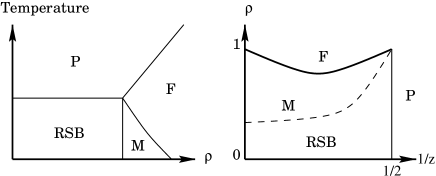
FIG. 1.: Left: Phase diagram in a mean-field model ($\rho$ is the excess concentration of ferromagnetic bonds, c.f. eq. 1). A mixed (M) phase, with both ferromagnetic (F) ordering and replica symmetry breaking (RSB), is present. At larger temperature the system is paramagnetic (P). Right: The role of the coordination on the presence of such a mixed phase in the mean field picture at temperature $T=0$ (artist’s view).

Theoretical expectations —

In the mean field picture, based on the infinite range Sherrington-Kirkpatrick (SK) model [7], one has the following sequence at low temperature when the concentration of ferromagnetic interactions is increased (see Fig. 1): (a) an RSB phase with no magnetization ($m=0$); (b) a “mixed” phase with both RSB and $m>0$; (c) a standard ferromagnetic phase. The same phase diagram arises in the Random Energy Model [8]. In these models the mixed phase follows from the existence of a spin glass phase in a magnetic field; indeed, a non zero magnetization creates an effective magnetic field, and thus mixed phases seem unavoidable in mean field. One can also consider finite connectivity generalizations [9, 10] of the SK model where a spin is connected at random to a finite number of other spins. A study of the associated phase diagram has been performed [11] for connectivity $3$ and again shows the presence of a mixed phase, while the limit of large connectivities brings us back to the SK model. Now the combination of spin glass ordering and very low connectivity most likely inhibits ferromagnetism, so the size of the mixed phase should grow as the connectivity increases. This is what we illustrate in Fig. 1. If mean field is a good guide for three dimensions, then a mixed phase should be easier to observe on lattices with large connectivities; for this reason we shall consider lattices with next-nearest neighbor interactions.

Within the droplet or scaling theories, the phase diagram is very different because any magnetic field destroys the spin glass ordering. For instance, within the droplet picture [4], the mixed phase is incompatible with compact droplets. Similarly, within the scaling picture [5], having a mixed phase would require a line of neutral fixed points connecting two unstable fixed points under the renormalization group, i.e., highly singular and non generic flows. Not surprizingly, the absence of a mixed phase is explicitly confirmed in the Migdal-Kadanoff bond-moving approach [12, 13]. This picture works very well in low dimensions, and in particular it agrees with the consensus of no mixed phase in dimensions $d\leq 2$ [14, 15]. Our focus in this work is the case $d=3$ where the question of a mixed phase remains open. Note that high temperature series cannot address this problem as the mixed phase resides beyond the first boundary of singularities. A good way to tackle it is via Monte Carlo; unfortunately, such studies have systematically avoided the question of the mixed phase, focusing instead on ordering from the paramagnetic side. The only attempt to search for an equilibrium mixed phase we are aware of is that of Hartmann [6] who worked at zero-temperature but was not able to estimate precisely the boundary of the spin glass phase and thus made no claims about the existence or not of a mixed phase.

The models —

We consider Edwards-Anderson-like Hamiltonians on a $L\times L\times L$ cubic lattice:

$$H_{J}(\{S_{i}\})=(1-\rho)\sum_{<ij>}J_{ij}S_{i}S_{j}-\rho\sum_{<ij>}S_{i}S_{j}$$ (1)

where $S_{i}=\pm 1$ are Ising spins and $\rho$ controls the amount of frustration in the system. The sums are over all nearest neighbor spins in the First Neighbor Model (FNM), and over nearest and next-nearest neighbor spins (a total of $18$) in the Second Neighbor Model (SNM). The quenched couplings $J_{ij}$ are independent random variables, taken from a Gaussian distribution of zero mean and unit variance and we impose periodic boundary conditions. This Hamiltonian has both a spin glass term and a ferromagnetic term; for $\rho=0$ we recover the standard spin glass model while for $\rho=1$ we have the usual Ising ferromagnet. We use sizes up to $L=12$ for the FNM and up to $L=8$ for the SNM. At these sizes, the heuristic algorithm [16] we use gives the ground state with very high probability so that our systematic errors are much smaller than our statistical ones.

Ferromagnetic ordering —

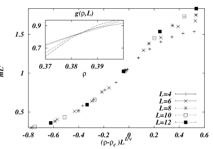
FIG. 2.: Scaling plot of $m$ as a function of $\rho$ in the First Neighbor Model; ${\rho}_{F}=0.385$, $\nu=0.9$ and $\beta=0.3$. The inset shows the Binder cumulant of $m_{J}$.

We first focus on the transition from a state where the magnetization per spin $m$ is zero to a ferromagnetic state ($m\neq 0$). Note that the Hamiltonian has the global symmetry $\{S_{i}\}\to\{-S_{i}\}$, so $m$ is an order parameter for the transition. For each instance, we determine the magnetization density $\pm m_{J}$ (since the $J_{ij}$ are independent continuous random variables, there are only two ground states, related by symmetry). Our order parameter is then

$$m=\left[{\overline{m_{J}^{2}}}~{}\right]^{1/2}$$ (2)

where ${\overline{~{}\cdot~{}}}$ denotes the average over the disorder variables $\{J_{ij}\}$.

For a large excess of ferromagnetic interactions ($\rho\approx 1$), $m$ will be close to $1$, while for a small excess ($\rho\approx 0$), $m$ will go to zero in the large volume limit.

FIG. 3.: Scaling plot of the mean value of $m$ as a function of $\rho$ in the Second Neighbor Model; ${\rho}_{F}=0.236$, $\nu=0.9$ and $\beta=0.3$. The inset shows the Binder cumulant of $m_{J}$.

For both the FNM and SNM, the transition appears to be of second order; indeed our distributions of $|m_{J}|$ always have a single peak whereas a first order transition should lead to two peaks at the transition point, one at $m>0$ and one at $m=0$. (These two peaks would be generated by those samples that are magnetized and those that are not.) To determine the critical value $\rho_{F}$, we have computed the Binder cumulant associated with the distribution of $m_{J}$:

$$g\left(\rho,L\right)={\frac{1}{2}}\left(3-{\frac{\overline{m_{J}^{4}}}{{\overline{m_{J}^{2}}}^{2}}}\right).$$ (3)

The different $L$ curves cross very well for both models, giving ${\rho}^{FNM}_{F}=0.385(5)$ and ${\rho}^{SNM}_{F}=0.236(5)$. Moreover, applying finite size scaling, we should have $g\left(\rho,L\right)={\tilde{g}}\left(L^{1/\nu}\left(\rho-\rho_{F}\right)\right).$ Doing so for the order parameter, we expect $m\left(\rho,L\right)=L^{-\beta/\nu}F\left(L^{1/\nu}\left(\rho-\rho_{F}\right)\right)$. The corresponding data collapse is very satisfactory as can be seen in Fig. 2 and 3. Furthermore, the values of the critical exponents are close for the two models: we find $\beta=0.3(1)$ and $\nu=0.9(2)$. These values are within the error bars of those found by Hartmann who studied the case where $J_{ij}=\pm 1$ [6], obtaining $\beta=0.2(1)$ and $\nu=1.1(3)$. Last but not least, the values of the Binder cumulant at the critical point are all close to one-another. These results give evidence in favor of universality in spin glasses, at least for this particular transition.

Replica symmetry breaking and sponges —

RSB literally means that $P(q)$, the probability distribution of spin overlaps taken between equilibrium configurations is not concentrated as in a ferromagnet. Unfortunately, estimations of $P(q)$ are plagued by finite size effets. Hartmann [6] measured the width of $P(q)$ among ground states of the $\pm J$ model but, because of subtleties intrinsic to that model, he was not able to determine the location of the spin glass phase boundary and thus made no claims about the existence of a mixed phase. In our work we use a different probe of RSB that seems to suffer far less from finite size effects. The starting point is to remark that in the presence of RSB several macroscopically different valleys dominate the system’s partition function, having $O(1)$ differences in free-energy. Extrapolating such behavior to zero-temperature, we expect to have system-size excitations above the ground state costing only $O(1)$ in energy. In our models, we characterize the system-size excitations by their topology, following the procedures developped in [17]. First, we produce an excitation by taking at random $2$ spins in the ground state, forcing them to change their relative orientation, and recomputing the new ground state with that constraint. By definition, the spins that are flipped in an excitation form a connected cluster; if it and its complement “wind” around in all three $(x,y,z)$ directions, we call it a sponge. (For instance a cluster winds in the $x$ direction if there exists a closed walk on it having non-zero winding number in $x$.) We use the proportion of such sponge-like (topologically non-trivial) events as an order parameter for RSB. In the droplet model, this quantity decays as $L^{-\theta}$ so asymptotically there are no large scale $O(1)$ excitations. As in [17], we increased the signal to noise ratio by first ranking the spins according to their local field; then we took the two spins at random from the list’s top $25\%$ (or $50\%$, both led to the same conclusions).

We have measured this order parameter as a function of $\rho$ and $L$. Our results are very similar in the FNM and the SNM. Looking at the plot in Fig. 4, there seems to be a phase transition in the FNM at ${\rho}^{FNM}_{RSB}\approx 0.380(5)$. Fitting these curves leads unambiguously to a non-zero large $L$ value for the order parameter when ${\rho}=0.37$ and to a zero value when ${\rho}=0.39$. In the SNM (see inset of Fig. 4), we find ${\rho}^{SNM}_{RSB}\approx 0.235(5)$ and the extrapolations away from this point behave as in the FNM. Note that, within statistical errors, the curves have a common crossing point. Furthermore, just as for $\rho=0$, up to the transition point the fraction of sponge-like events increases with $L$. It thus seems most likely that these excitations survive as $L\to\infty$ if $\rho<\rho_{RSB}$. This is as expected in the mean field approach, but not in the droplet/scaling pictures.

FIG. 4.: Fraction of sponge-like excitations versus $\rho$ in the FNM. (The inset shows the data for the SNM.) ${\rho}^{FNM}_{{RSB}}=0.380(5)$ (${\rho}^{SNM}_{{RSB}}=0.235(5)$).

However, the transition point ${\rho}_{\rm{RSB}}$ is close if not equal to ${\rho}_{\rm{F}}$ in both of our models, so it seems to us that there is no mixed phase having both sponge excitations and positive magnetization. This would be in contrast to the mean field prediction.

Domain wall wandering and ${\theta}_{\rm{DW}}$ —

We now study directly the spin glass ordering, be-it with or without RSB, so we no longer resort to $O(1)$ energy sponges. It is well known that spin glass ordering is sensitive to perturbations; the standard probe for this consists in comparing periodic and anti-periodic boundary conditions [5], thereby creating an interface in the system. The typical energy change for such a modification of boundary conditions should grow more slowly than $L^{2}$ in the spin glass phase, with $O(1)$ energy changes arising not too rarely, for instance with a probability going as an inverse power of $L$. Another important aspect of such an interface is associated with its position space properties: in a spin glass phase, it is “space spanning”. This can be made precise algorithmically by considering whether the interface winds around the whole lattice. We take this behavior to be an indication of the “fragility” of the ground state; we thus consider that we are in a spin glass phase when there is a positive probability that the interface is “spongy”, i.e., winds around the lattice.

We begin with the FNM. In Fig. 5 we show the fraction of instances where the interface is spongy.

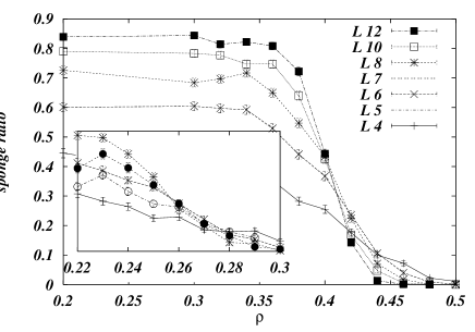
FIG. 5.: Fraction of spongy interfaces versus $\rho$ in the FNM. (The inset shows the data for the SNM.) The crossing points drift to the left, suggesting ${\rho}_{\rm{DW}}\approx{\rho}_{\rm{RSB}}$.

The data suggest a transition at ${\rho}_{\rm{DW}}{\leq}0.4$. However there is a systematic drift of the crossing points to the left so the most straight-forward interpretation of our results is ${\rho}_{\rm{RSB}}={\rho}_{F}={\rho}_{\rm{DW}}$; then the spin glass ordering disappears when the ferromagnetic ordering appears, the two orderings do not co-exist and there is no mixed phase.

If on the other hand one really believes mean field to be a good guide, one can assume that the mixed phase is present but only in a very small window, something like ${\rho}\in[0.38,0.40]$. To make such a window larger and thus to give creadence in favor of a mixed phase, we increase the connectivity of the lattice from $6$ to $18$ by going to the SNM. There, our analysis leads to ${\rho}_{\rm{DW}}\leq 0.255$; thus in this “improved” model, the most optimistic estimate for the window would be ${\rho}\in[0.236,0.255]$. However just as in the FNM, the crossing points of the curves drift and again ${\rho}_{\rm{DW}}-{\rho}_{\rm{RSB}}$ is very small if not zero, a result quite puzzling from the mean field perspective, not to mention the fact that RSB seems to be excluded in this window.

To pursue the search for a mixed phase, we have studied the FNM in $d=4$ for sizes $L\leq 5$. The behavior is similar to the case $d=3$, and in particular we obtain ${\rho}_{F}=0.315(5)$ and ${\rho}_{\rm{RSB}}=0.325(5)$ (data not shown). But the crossing points of the Binder cumulant which determine ${\rho}_{F}$ now shift towards larger values as $L$ increases. As a result, there is no compelling evidence for a mixed phase and probably $\rho_{DW}=\rho_{F}=\rho_{RSB}$.

Discussion and conclusions —

In spite of our attempts to render finite dimensional models mean-field-like, we are unable to confirm the mean field prediction that RSB and ferromagnetic order can co-exist. Since we also find quite clear signals for RSB via the existence of spongy clusters having $O(1)$ energies in the whole unmagnetized region, we cannot explain our results using the droplet/scaling theories either. (There is no RSB in those approaches.) Interestingly, all the results we obtain are compatible with the “Trivial-Non-Trivial” or TNT picture [17, 18]. In that picture, there are system-size excitations whose energies are $O(1)$; this leads to RSB, i.e. a non-trivial distribution of spin overlaps. Furthermore, they are also compact, with a surface fractal dimension $d_{s}<d$, leading to a trivial distribution of link overlaps. This TNT picture forbids a mixed phase as follows. Assume that the local magnetization density (in a big enough sub-volume of the whole) is self-averaging and equal to the global magnetization density. Activating compact system-size excitations will not affect the local magnetization but will change the global one unless $m=0$. A well behaved magnetization with TNT then forces $m=0$, i.e., no mixed phase.

Other numerical studies, in particular based on Monte-Carlo simulations, are needed. On the analytical side, a computation of the phase diagram on the Bethe lattice with RSB [19], or field theoric approaches for the mixed phase in the spirit of [20], would be welcome. Finally, experimentally, it may be possible to test whether magnetization and spin glass ordering can co-exist in equilibrium; however this will require careful checks that equilibrium is indeed reached.

REFERENCES

- [1] Spin Glasses and Random Fields, edited by A. P. Young (World Scientific, Singapore, 1998).
- [2] M. Mézard, G. Parisi, and M. A. Virasoro, Spin-Glass Theory and Beyond, Vol. 9 of Lecture Notes in Physics (World Scientific, Singapore, 1987).
- [3] E. Marinari et al., J. Stat. Phys. 98, 973 (2000).
- [4] D. S. Fisher and D. A. Huse, Phys. Rev. Lett. 56, 1601 (1986).
- [5] A. J. Bray and M. A. Moore, in Heidelberg Colloquium on Glassy Dynamics, Vol. 275 of Lecture Notes in Physics, edited by J. L. van Hemmen and I. Morgenstern (Springer, Berlin, 1986), pp. 121–153.
- [6] A. Hartmann, Phys. Rev. B 59, 3617 (1999).
- [7] D. Sherrington and S. Kirkpatrick, Phys. Rev. Lett. 35, 1792 (1975).
- [8] B. Derrida, Phys. Rev. B 24, 2613 (1981).
- [9] L. Viana and A. J. Bray, J. Phys. C 18, 3037 (1985).
- [10] C. de Dominicis and Y. Goldschmidt, J. Phys. A Lett. 22, L775 (1989).
- [11] C. Kwon and D. J. Thouless, Phys. Rev. B 37, 7649 (1988).
- [12] A. P. Young and B. W. Southern, J.Phys.C 10, 2179 (1977).
- [13] G. Migliorini and A. N. Berker, Phys. Rev. B. 57, 426 (1998).
- [14] N. Kawashima and H. Rieger, Europhys. Lett. 39, 85 (1997).
- [15] H. Nishimori, Statistical Physics of Spin Glasses and Information Processing: An Introduction (Oxford University Press, Oxford, UK, 2001).
- [16] J. Houdayer and O. C. Martin, Phys. Rev. E 64, 056704 (2001).
- [17] F. Krzakala and O. C. Martin, Phys. Rev. Lett. 85, 3013 (2000).
- [18] M. Palassini and A. P. Young, Phys. Rev. Lett. 85, 3017 (2000).
- [19] M. Mézard and G. Parisi, Eur. Phys. J. B 20, 217 (2001).
- [20] I. R. Pimentel, T. Temesvari, and C. D. Dominicis, Phys. Rev. B 65, 224420 (2002).