Ising magnets with mobile defects

Abstract

Motivated by recent experiments on cuprates with low-dimensional magnetic interactions, a new class of two–dimensional Ising models with short–range interactions and mobile defects is introduced and studied. The non–magnetic defects form lines, which, as temperature increases, first meander and then become unstable. Using Monte Carlo simulations and analytical low– and high–temperature considerations, the instability of the defect stripes is monitored for various microscopic and thermodynamic quantities in detail for a minimal model, assuming some of the couplings to be indefinitely strong. The robustness of the findings against weakening the interactions is discussed as well.

I Introduction

Low–dimensional magnetism in high-$T_{c}$ superconductors has attracted much interest, both theoretically and experimentally Review . In particular, striped structures in magnets derived from the $La_{2}CuO_{4}$ compound have been discussed rather extensively. Motivated by related analyses and, more specifically, by recent experiments Buch on $(Sr,Ca,La)_{14}Cu_{24}O_{41}$, we shall introduce a novel class of quite simple two–dimensional Ising models, mimicing $Cu^{2+}$ ions by spin-1/2 Ising variables and holes by non–magnetic defects ($S$= 0). Of course, the aim of the present study is not to offer a full, or partial explanation of the experimental subtleties. Indeed, beyond the experimental motivation, the model is hoped and believed to show various intriguing properties being of genuine theoretical interest.

locatWe consider the situation where the spins are arranged in chains, with antiferromagnetic interactions, $J_{a}$, between adjacent chains, and a ferromagnetic coupling, $J$, between neighbouring spins in the chains, augmented by an antiferromagnetic coupling, $J_{0}$, between next–nearest spins in the same chain with a defect in between them. The defects are allowed to move through the crystal, along the chains.

The defects tend to form stripes, perpendicular to the chains, which, for increasing temperature, first meander and then become unstable. To identify the impact of the defect mobility on the stripe instability, a ’minimal model’ is proposed by assuming indefinitely strong interactions in the chains, $J$ and $J_{0}$. This model is studied analytically, at low and high temperatures, and, for a wide range of temperatures, by using standard Monte Carlo techniques Binder . Contact will be made to well known descriptions of wall instabilities in two dimensions, as have been put forward, for instance, in the context of incommensurate superstructures in two dimensions Pokro and step roughening on vicinal surfaces Villain . Deviations from these standard scenarios will be discussed.

To study the robustness of the properties of the minimal model and to identify other possibly interesting aspects of this class of Ising models as well, we also considered cases with finite couplings in the chains. In addition, both for the minimal model and the ’full model’, the effect of an external magnetic field has been investigated.

The paper is organized accordingly. In the next section, we introduce the model and elucidate its experimental background. Then, we present our results on the minimal model, followed by a discussion on properties of the full model. A short summary concludes the article.

II Models and methods

We consider Ising models on a square lattice, setting the lattice constant equal to one. Each lattice site $(i,j)$ is occupied either by a spin, $S_{i,j}=\pm 1$, or by a defect corresponding to spin zero, $S_{i,j}=0$. The defects are assumed to be mobile along one of the axes of the lattice, which will be called the chain direction in the following. Neighbouring sites of the same chain, $(i,j)$ and $(i\pm 1,j)$, are not allowed to be occupied both by defects (short range repulsion between defects). The mobility of a defect may be influenced by a pinning potential, which, however, will be disregarded in most of the following analysis. Even for vanishing pinning, the defect cannot diffuse freely, in general, because an elementary move, characterized by exchanging a defect and a, possibly flipped spin at neighbouring sites, is affected by the magnetic interactions along and perpendicular to the chain direction. We assume a ferromagnetic coupling, $J>0$, between neighbouring spins, $S_{i,j}$ and $S_{i\pm 1,j}$, along the chain augmented by an antiferromagnetic interaction, $J_{0}<0$, between those next–nearest spins of the same chain, which are separated by a defect. Spins in adjacent chains, $S_{i,j}$ and $S_{i,j\pm 1}$, are coupled antiferromagnetically, $J_{a}<0$. Accordingly, the Hamiltonian of the model may be written as

$${\cal H}=-\sum\limits_{ij}(JS_{i,j}S_{i\pm 1,j}+J_{0}S_{i,j}S_{i\pm 2,j}(1-S_{i\pm 1,j}^{2})$$

$$+J_{a}S_{i,j}S_{i,j\pm 1})-H\sum\limits_{ij}S_{i,j}$$ (1)

where we included a field term. Note that the defects, $S_{ij}=0$, are separated, along the chains, by at least one spin. We shall assume that the number of defects is the same in each chain, determined by the defect concentration $\Theta$, denoting the total number of defects divided by the total number of sites.

The model describes, among others, the thermal distribution of defects, leading to rather intriguing properties, as will be shown below. In particular, at low temperatures, the defects tend to form stripes perpendicular to the chains which become unstable at higher temperatures. The model is believed to be of genuine theoretical interest.

The theoretical model may be motivated by rather recent experimental findings for the so called telephone number compound $(Sr,Ca,La)_{14}Cu_{24}O_{41}$ which contains two magnetically one-dimensional elements. One subsystem is a sheet like arrangement of $Cu_{2}O_{3}$ two-leg ladders, which is irrelevant in the context of the present paper. The second subsystem is an array of $CuO_{2}$ chains formed by edge sharing $CuO_{4}$ plaquettes. For this bond geometry with a $Cu-O-Cu$ bond angle close to 90 degree the Goodenough-Kanamori-Anderson rules predict a ferromagnetic exchange between nearest neighbour $Cu$ ions with spin $S=\frac{1}{2}$. This is confirmed by neutron diffraction studies of the magnetic structure in the ordered state which, in addition, show an antiferromagnetic coupling of the spins perpendicular to the chains Matsuda98 . To our knowledge the absolute value of the ferromagnetic coupling constant $J$ in the undoped chains has not been determined yet from inelastic neutron data. A mean field treatment of the magnetic susceptibility suggests a coupling constant of several meV Carter ; Buch .

A long range magnetic order of the $Cu$ spins is only observed for certain compositions of the telephone number compound. For many compositions the chains contain a large number of hole-like charge carriers. These holes imply non-magnetic $Cu$ sites Carter ; Ammerdimer ; KataevPRB which inhibit the formation of a long range ordered magnetic state. For example, in the stoichiometric compound $Sr_{14}Cu_{24}O_{41}$ about 60 percent of the $Cu$ sites in the chains are non-magnetic Osafune97 ; Regnault ; Nucker00 and the remaining spins form nearly independent dimers Regnault ; Ammerdimer . The analysis of this dimer state shows a rather large antiferromagnetic coupling $|J_{0}|\simeq 11$ meV between the two $Cu$ spins adjacent to a non-magnetic $Cu$ site Regnault ; Ammerdimer ; Remark1 . This coupling is about one order of magnitude larger than the antiferromagnetic coupling between $Cu$ ions in adjacent chains Regnault .

The experimental data mentioned so far yield at least three relevant magnetic coupling constants in the telephone number compounds: a ferromagnetic coupling $J$ of several meV between nearest neighbour $Cu$ ions in the chain, the antiferromagnetic $|J_{0}|\simeq 11$ meV for $Cu$ spins adjacent to holes Remark1 and an antiferromagnetic coupling $J_{a}$ between $Cu$ spins in adjacent chains which is of the order of 1 meV Regnault . For undoped chains the magnetic properties depend mainly on $J$ and $J_{a}$, whereas the behaviour for large hole content is determined by a single coupling constant, the antiferromagnetic exchange $J_{0}$. For small hole concentrations all three magnetic interactions and their interplay should be relevant. Experimentally such a situation is realized in $La_{5}Ca_{9}Cu_{24}O_{41}$ where the hole content in the chains amounts to about 10 percent Nucker00 . Studies of this compound reveal a very unusual suppression of the magnetic order in external fields which can not be explained in terms of conventional spin models Buch . It is tempting to attribute this strange behaviour to a magnetic field induced movement of the charge carriers which frustrates the antiferromagnetic interchain coupling.

As will be shown below our numerical results for the model Eq. (1) indeed reveal a movement of holes in external fields. We mention that the treatment within an Ising model is also related to experimental findings for the telephone number compound. Different experimental data for lightly doped chains show a strong Ising-like anisotropy Buch ; KataevPRL which was predicted by two independent theoretical treatments for spin chains formed by edge sharing $CuO_{4}$ plaquettes Aha .

To study the above Ising model with mobile defects, Eq. (1), we applied analytical low and high temperature considerations, and Monte Carlo techniques monitoring various thermodynamic and microscopic properties. In the simulations, we took into account flips of single spins as well as hops of a defect to a neighbouring site in the chain leaving a spin at the former defect site. Of course, simulations are performed on finite lattices with $L\times M$ sites ($L$ refers to the chain direction). Usually, we employed full periodic boundary conditions. In a few selected cases free boundary conditions perpendicular to the chain direction were applied, corroborating the results for periodic boundary conditions to be presented in the following. To investigate finite size effects, the linear dimensions, $L$ and $M$, were varied from 20 to 160. Typically, runs of at least $10^{6}$ Monte Carlo steps per spin were performed, averaging then over a few of such realizations to estimate error bars. The concentration of defects, $\Theta$, ranged from zero to 15 percent. In most cases, we set $\Theta=0.1$.

Physical quantities of interest include the specific heat, $C$, determined from energy fluctuations and the temperature dependence of the energy, the magnetization per site, $m$, and the correlation functions parallel, $G_{1}(r)=(\sum\limits_{ij}\langle S_{i,j}S_{i+r,j}\rangle)/LM$, and perpendicular, $G_{2}(r)=(\sum\limits_{ij}\langle S_{i,j}S_{i,j+r}\rangle)/LM$, to the chain direction. We also calculated other microscopic quantities describing the stability of the defect stripes and the ordering of the spins and defects in the chains. In particular, we computed the average minimal distance, $d_{m}$, between each defect in chain $j$, at position $(i,j)$, and those in the next chain, at $(i^{\prime},j+1)$ (i.e. $\sum\langle\min|i-i^{\prime}|\rangle$, dividing this sum over the defects by their number), the cluster distribution, $n_{d}(l)$, denoting the probability of a cluster with $l$ spins of equal sign in a chain (in analogy to the distribution of cluster lengths in percolation theory Stauffer ), and the normalized number of sign changes of neighbouring spins, $n_{c}$, in the chains. Finally, it turned out to be quite useful to visualize the microscopic spin and defect configurations as encountered during the simulation.

In case of the magnets mentioned above, the absolute values of both $J_{0}$ and $J$ are large compared to the coupling between chains, $J_{a}$. To describe then the behaviour of the Hamiltonian, Eq. (1), at low temperatures one may consider a simplified model in which the spins form intact clusters in the chains between two consecutive defects changing the sign at the defect, i.e. $J$ and $|J_{0}|$ are assumed to be indefinitely strong. Quantities can now be expressed in terms of $k_{B}T/|J_{a}|$. The thermal excitations are due to motion of the defects in the chains. Again, defects are separated by at least one spin. The analysis of this ’minimal model’ will be presented in the next section.

III Properties of the minimal model

III.1 Monte Carlo results

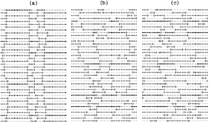
Figure 1: Typical Monte Carlo equilibrium configurations of the minimal model, $\Theta=0.1$and $H=0$, of size $L=M=$ 40 at temperatures $k_{B}T/|J_{a}|$= 0.6 (a), 2.6 (b), and 4.0(c).

Figure 2: Cluster distribution $n_{d}(l)$ at $k_{B}T/|J_{a}|$= 0 (circles), 0.5 squares, 1.0 (diamonds), 1.5 (triangles up), 2.5 (triangles left), and 4.0 (triangles down), for the minimal model, $\Theta=0.1$, and $H=0$, of size $L=M=40$. Results have been obtained by exact enumerations at zero temperature, and by simulations otherwise.

In the ground state of the minimal model with vanishing external field, $H=0$, the defects form straight lines perpendicular to the chains and separating antiferromagnetic domains of spins. The ground state is highly degenerate, with the degeneracy depending on the concentration $\Theta$ of defects. Each arrangement of straight defect lines, with a separation distance between the lines of at least two lattice spacings, has the same, lowest possible energy, resulting in a fast decay of the correlations $G_{1}$ parallel to the chains, while the spins are perfectly correlated perpendicular to the chains. The degeneracy may be (partly) lifted, for instance, by introducing a pinning potential or by applying an external field as will be discussed briefly below.

Increasing the temperature, $T>0$, the defects are allowed to move so that the stripes start to meander and finally break up, as exemplified in typical Monte Carlo configurations depicted in Fig. 1. It seems plausible that the destruction of the defect stripes by thermal fluctuations is accompanied by singular behaviour of thermodynamic quantities, like the specific heat, and various correlations functions. This suggestion is, indeed, supported by the numerical evidence discussed below. The effect of both phenomena, meandering and breaking up of the stripes, on various physical quantities are shown in Figs. 2 to 6, for the case $\Theta=0.1$. Note that in most of the figures we did not include error bars being, typically, not larger than the size of the symbols.

At low temperatures, deviations from the straight stripes may be characterised by kinks and kink–antikink pairs Pokro ; Villain ; Pers ; Selke. Actually, the minimal model resembles closely a terrace–step–kink (TSK) model describing step fluctuations on vicinal surfaces. The energies of the elementary excitations may be readily calculated. For instance, a kink with depth of one lattice spacing costs $-J_{a}$, a kink–antikink pair, created by moving a single defect by one site away from the perfect stripe, costs $-2J_{a}$, for a further diffusion of that defect by another lattice spacing away from the stripe an additional $-4J_{a}$ is needed, etc. The fact that consecutive defects in a chain cannot be closer than the minimum distance of two lattice spacings leads to the well known phenomenon of ’entropic repulsion’ Mullins ; Pers between meandering neighbour stripes. Due to the entropic repulsion, the meandering stripes tend to approach their average distance as given by the concentration of defects, $\Theta$ (here, at $\Theta=0.1$, the average distance is ten lattice spacings). This feature is seen, e.g., in the thermal behaviour of the cluster distribution, $n_{d}(l)$, where the distance between two neighbouring defects in a chain is, in the minimal model, equal to $(l+1)$. As shown in Fig. 2 for the moderate size $L=M=40$, at zero temperature, $n_{d}(l)$, calculated numerically by taking into account all degenerate ground states, decreases monotonically with the separation distance $l$. When turning on the temperature, the maximum of $n_{d}(l)$ moves towards equidistant spacing of defects, here $l=9$, and the shape of $n_{d}(l)$ may be approximated by a Gaussian or Wigner function, as has been discussed recently in the context of terrace width distributions for vicinal surfaces Einstein . Increasing the temperature furthermore, $T\longrightarrow\infty$, the defects take random positions in the chains, and $n_{d}(l)$ acquires, of course, again the same Poissonian form as at $T=0$ for random distribution of defect lines. The destabilization of the stripes is indicated, for example, by a rather rapid decrease, with temperature, of the probability to find defects at their average spacing, i. e. $n_{d}(l=9)$ for $\Theta=0.1$, see Fig. 5.

Figure 3: Parallel correlation function $G_{1}(r)$ at $k_{B}T/|J_{a}|$= 0 (circles), 0.5 (squares), 1.0 (diamonds), 1.5 (triangles up), 2.0 (triangles left), and 2.5 (triangles down), for the minimal model of size $L=M=60$, as obtained from exact enumeration, $T=0$, and simulations otherwise.

As depicted in Fig. 3, meandering and breaking up of the stripes may be also observed in the correlation function parallel to the chains, $G_{1}(r)$. Again, the behaviour at zero temperature has been determined numerically without difficulty, for fairly small system sizes, by averaging over all ground states. The correlations are seen to decay rapidly. The oscillations in $G_{1}(r)$, already hardly visible for $L=60$, as shown in Fig. 3, become less and less pronounced when enlarging $L$ at fixed $\Theta(=0.1)$. The asymptotics of $G_{1}(r)$, for large $L$, may be determined analytically, as discussed in the following subsection. Raising now the temperature, $T>0$, the correlations first become stronger, reflecting the ordering tendency which favour equidistant stripes due to the entropic repulsion, and then decrease quite drastically due to the thermal destabilization of the stripes. In fact, the perpendicular correlations, $G_{2}$, fall off rather rapidly in the same range of temperatures. Finally, when $T\longrightarrow\infty$, one encounters again the behaviour at zero temperature, with the defects at random positions.

Figure 4: Distance between defects in adjacent rows $d_{m}(T)$, simulating the minimal model of size $L=M=20$ (circles), 40 (squares), 60 (diamonds) and 80 (triangles up).

The destruction of the defect stripes is detected directly in the average minimal distance between defects in adjacent chains, $d_{m}$. Obviously, $d_{m}$ is equal to zero at $T=0$, and $d_{m}\approx 2\exp(-|J_{a}|/k_{B}T)$ at low temperatures, $k_{B}T\ll|J_{a}|$. In Fig. 4, data for various system sizes, $L=M$ ranging from 20 to 80, are displayed. While at low temperatures, $d_{m}(T)$ does not depend, in fact, significantly on the system size, it starts to rise rapidly at some characteristic temperature, with the height of the maximum in the temperature derivative of $d_{m}$ increasing strongly with larger system size. The location of the maximum, at $T_{d}^{max}$, signalling the breaking up of the stripes, moves to lower temperatures as $L$ gets larger. The quantitative behaviour is quite similar to the one of the specific heat, to be discussed below.

Figure 5: Temperature and size dependence of probability for next–nearest neighbour pairs of defects, $n_{d}(l=1)$ (open symbols) and pairs at average distance $n_{d}(l=9)$ (full symbols), simulating systems of size $L=M$= 20 (circles), 40 (squares), and 60 (diamonds).

One possible reason for the destabilization of the stripes are effectively attractive interactions between neighbouring defects or lines, mediated by the spins. Indeed, such an interaction may occur, for instance, for strongly fluctuating stripes so that three consecutive defects in one chain, $j$, are in the cage formed by pairs of defects in the adjacent chains, $j\pm 1$. Consequently, two of the three defects tend to form a pair of next–nearest neighbouring defects, as may be checked easily. In any event, the probability of such pairs of defects is obviously given by $n_{d}(l=1)$. Its temperature and size dependence is depicted in Fig. 5 (together with that of $n_{d}(l=9)$, as mentioned above), showing a drastic increase close to the characteristic temperature of the breaking up of the stripes, $T_{d}^{max}$. Note that this type of stripe instability is not included in the standard descriptions of wall instabilities in two dimensions Pokro ; Villain ; Pers ; Halperin , where either the number of walls is not fixed, giving rise to incommensurate structures, or dislocations play a crucial role, in the context of melting of crystals. Also the bunching of steps in TSK models with attractive step–step interactions Weeks or instabilities in polymer filaments due to attractive couplings Lipo ; Burk are quite different from the loss of stripe coherency we observe here. Of course, the breaking up of the stripes has to be distinguished from their meandering which may result in their roughness, driven by capillary wave excitations Villain .

Figure 6: Specific heat, $C$, for systems of size $L=M=$ 20 (circles), 40 (squares), and 80 (diamonds).

Figure 7: Size dependence of the location of the maximum in the specific heat, $T_{C}^{max}(L)$, as obtained from simulations of the minimal model, $\Theta=0.1$ and $H=0$, for $L=M=$ 20, 40, 60, 80, 100, and 160.

Meandering and destabilization of the stripes also show up in the specific heat, $C$, see Fig. 6 for systems with $L=M$ sites, $L$ ranging from 20 to 80. For each size, $C$ exhibits two maxima. The maximum at the lower temperature is almost independent of the system size, and it is related to the kink excitations of the stripes. The upper maximum, occurring at $T_{C}^{max}(L)$, signals the instability of the defect stripes. Its height increases with increasing system size, indicating possibly a phase transition in the thermodynamic limit, $L\longrightarrow\infty$. To estimate the transition temperature, we plotted $T_{C}^{max}$ versus $1/L$, with $L$ going up to 160, see Fig. 7. From a linear extrapolation we obtain approximately $k_{B}T_{C}^{max}(L=\infty)/|J_{a}|=1.05\pm 0.05$. Note that finite size analyses, usually for sizes up to 80, for other quantities, like $G_{1}$, $G_{2}$, and $n_{d}(l=9)$, lead to similar estimates for the possible transition temperature. However, the close agreement may be fortuituous, depending on the type of the transition. For instance, for a Kosterlitz–Thouless transition, the peak in the specific heat does not occur exactly at the transition temperature, as $L\longrightarrow\infty$. A detailed analysis of this subtle feature is, however, beyond the scope of the present study.

From simulations of the minimal model with $\Theta=0.05$ and $\Theta=0.15$, $L=M=40$, we infer that the characteristic temperature, at which the stripes become unstable, gets smaller when the concentration of defects, $\Theta$, is increased. This observation may be explained by the fact that the effectively attractive interactions, caused, for instance, by the cage effect described above, may set in obviously at lower temperature when the average distance between the stripes decreases.

Applying an external field, $H>0$, the ground states change when $H$ exceeds specific critical values. For $|2J_{a}|>H>|J_{a}|$, the stripes are no longer straight, but they form a zig–zag structure. In that structure, supposing the field favours the ’+’ spins, each ’+’ cluster comprises two more spins than the ’$-$’ clusters directly below and above that cluster in the two adjacent chains. Defects bounding these ’$-$’ clusters are located exactly below and above the first and last spins of the ’+’ cluster. Spins and defects in each second chain are arranged identically. Obviously, the zig–zag structures carry a non–vanishing net magnetization. The degeneracy of the ground state is still high, albeit somewhat smaller than in the case of straight stripes at $H<|J_{a}|$, because the minimum length of ’+’ clusters is now three, instead of one. For larger fields, $H>2|J_{a}|$, the ’$-$’ clusters shrink drastically: ’$-$’ spins occur only in the pairs of next–nearest neighbouring defects; all other spins point in the direction of the external field.

Monitoring various quantities at fixed defect concentration, $\Theta=0.1$, the stripes are observed to become unstable at lower temperatures for stronger fields, $0<H<2|J_{a}|$. Varying the field at fixed small temperature, for the same defect concentration, we found, that the destruction of the stripes seems to be accompanied by a fairly rapid increase in the magnetization, $m$, leading to an anomaly in the field derivative of the magnetization, similar to experimental findings on $(Sr,Ca,La)_{14}Cu_{24}O_{41}$ Buch . The change from straight to zig–zag stripes, on the other hand, leads to a jump in $m(H)$ at $H=|J_{a}|$ and $T=0$. The corresponding maximum in the field derivative of the magnetization is, however, extremely weak already at very low temperatures. More detailed investigations are needed to clarify the experimental relevance of these observations. They are beyond our present scope.

The high degeneracy of the ground states may be lifted by introducing a pinning potential. For example, in related simulations for $H=0$, we found that meandering and breaking up of the stripes seem to be qualitatively not affected by a weak one–dimensional, along the chain direction, harmonic regular pinning potential. More realistically, one may introduce a random pinning potential. If it is sufficiently strong, it is expected to destroy the defect lines even at zero temperature. In a weak random potential, the coherency of the defect lines gets lost or the lines collide only on a large spatial scale, the ’Larkin length’ Larkin . At some finite temperatures, the collision length between neighbouring lines due to thermal fluctuations becomes smaller than the Larkin length. Starting from this temperature, the random pinning potential can be neglected in thermodynamics, though, it can be dominant for dynamic phenomena. Thus, our model is thermodynamically robust with respect to weak random potential except of a very low temperature region, in which probably a glassy state occurs.

III.2 Analytical results

Here we derive the asymptotics of the spin correlation functions in the chains, $G_{1}(r)=\langle S_{i,j}S_{i+r,j}\rangle$, for sufficiently large distances $r$, first at zero temperature, also valid at infinite temperature, and then at non–vanishing, but small temperatures. We start with the obvious statement that

$$S_{i,j}S_{i+r,j}=(-1)^{n_{0}(i,i+r)}$$ (2)

where $n_{0}(i,i+r)$ is the number of defects or ’zeros’, in the interval $(i,i+r)$. Eq. (2) can be rewritten as

$$S_{i,j}S_{i+r,j}=(e^{i\pi n_{0}(i,i+r)}+e^{-i\pi n_{0}(i,i+r)})/2$$ (3)

Assuming that $\langle n_{0}(i,i+r)\rangle=\bar{n}_{0}(r)$ is sufficiently large, we apply the Gaussian statistics to the deviation $\delta n_{0}(r)=n_{0}(i,i+r)-\bar{n}_{0}(r)$. Thus, the asymptotic expression of the correlation function reads

$$G_{1}(r)\approx\cos\pi\bar{n}_{0}(r)\exp\left(-\frac{\pi^{2}}{2}\langle(\delta n_{0}(r))^{2}\rangle\right)$$ (4)

The average $\bar{n}_{0}(r)$ is related to the concentration of zeros $c_{0}=\Theta$ by $\bar{n}_{0}(r)=c_{0}r$. The calculation of $\langle\left(\delta n_{0}(r)\right)^{2}\rangle$ is more tricky. First we calculate, at zero temperature, the probability $p(n_{0},r)$ of a fixed value of $n_{0}$ at fixed $r$. We find, disregarding here the value of the minimal distance between defects,

$$p(n_{0},r)=\exp(-r(c\ln\frac{c_{0}}{c}+(1-c)\ln\frac{1-c_{0}}{1-c}))/$$

$$\sqrt{2\pi rc(1-c)}$$ (5)

with $c=n_{0}/r$. For large numbers, the probability (5) has the Gaussian form near the maximum leading to the final result:

$$\langle(n_{0}-\bar{n}_{0}(r)^{2}\rangle=rc_{0}(1-c_{0})$$ (6)

Plugging this expression into Eq. (4), we obtain the asymptotics of $G_{1}(r)=\langle S_{i,j}S_{i+r,j}\rangle$ at zero temperature

$$G_{1}(r,T=0)\approx\cos(\pi c_{0}r)\exp\left(-\frac{\pi^{2}}{2}c_{0}(1-c_{0})r\right)$$ (7)

The asymptotics is valid for $r\gg r_{c}$, with the correlation length $r_{c}=2/(\pi^{2}c_{0}(1-c_{0})$. The condition of having a minimal distance of $q+1$ spacings between consecutive defects can be taken into account by replacing $c_{(0)}$ by $c_{(0)}/(1-c_{(0)}q)$. For our model $q=1$.

Note that the above considerations hold also in the high–temperature limit, $T\longrightarrow\infty$, as mentioned before.

At finite, but small temperatures, $k_{B}T\ll|J_{a}|$, the long–distance asymptotics of the correlation function $G_{1}(r)$ changes dramatically due to the meandering of the defect stripes. This process may be described by the free–fermion approximation Pokro . In this approach the lines are represented as trajectories of free fermions. Their entropic repulsion is treated as statistical repulsion of the fermions. The meandering of the lines means that, going from one moment of discrete time to the next one, each fermion can move to the left or right by one site with the amplitude (or probability) $z=\exp(-2|J_{a}|/k_{B}T)$. These processes are described by the Hamiltonian

$${\cal H}=-z\sum\limits_{i}(a^{+}_{i+1}a_{i}+a^{+}_{i}a_{i+1})$$ (8)

where the fermion operators $a_{i}$ and $a^{+}_{i}$ obey cyclic bondary conditions $a^{(+)}_{i+L}$= $a^{(+)}_{i}$. The Hamiltonian is diagonalized by Fourier transformation

$${\cal H}=-2z\sum\limits_{p}(\cos p)\alpha^{+}_{p}\alpha_{p};$$

$$p=2\pi m/L(m=1,2,...L)$$ (9)

where

$$a_{k}=\sum\limits_{p}e^{ipk}\alpha_{p}/\sqrt{L}$$ (10)

The energy band in $p$–space extends from $-\pi$ to $\pi$, but it is filled only partly, from $-p_{F}$ to $p_{F}$, where $p_{F}=\pi c_{0}$ (to take into account the specific minimal distance between defects, $c_{0}$ has to be substituted here and in the following as before). It means that in the ground state $\langle\alpha^{+}_{p}\alpha_{p}\rangle=1$ for $|p|=p_{F}$, and $\langle\alpha^{+}_{p}\alpha_{p}\rangle$= 0 for $p_{F}<|p|<\pi$. In this approach the number of zeros between $i$ and $i+r$ is given in terms of the fermion operators by

$$n_{0}(i,i+r)=\sum_{k=i}^{i+r}a^{+}_{k}a_{k}$$ (11)

The average of this quantity is obviously equal to $rc_{0}$, as at zero temperature, but its variance, $\langle\delta n^{2}\rangle=\langle(n_{0}(r)-\bar{n}_{0}(r))^{2}\rangle$, is drastically different. Indeed,

$$\langle\delta n^{2}\rangle=\sum_{k,k^{\prime}=i}^{i+r}\langle:a^{+}_{k}a_{k}::a^{+}_{k^{\prime}}a_{k^{\prime}}:\rangle$$ (12)

where :$XY$: denotes the normal product of the operators $X$ and $Y$. Applying the Wick theorem, one obtains

$$\langle\delta n^{2}\rangle=\sum_{k,k^{\prime}=i}^{i+r}\langle a^{+}_{k}a_{k}^{\prime}\rangle\langle a_{k}a^{+}_{k^{\prime}}\rangle$$ (13)

with the same summation limits. The diagonal term of this sum, $k=k^{\prime}$, gives the contribution $rc_{0}(1-c_{0})$, as at zero temperature. However, it will be completely compensated by the non–diagonal terms. Indeed, the simultaneous correlation function for free fermions is known LL to be equal to

$$\langle a_{k}a^{+}_{k^{\prime}}\rangle=\sin(p_{F}(k-k^{\prime}))/(\pi(k-k^{\prime}))$$ (14)

It is easy to check that $\langle a_{k}a^{+}_{k^{\prime}}\rangle=-\langle a^{+}_{k}a_{k^{\prime}}\rangle$. In the limit of small $p_{F}$, the summation in Eq.(13) can be replaced by an integration, which can be explicitly performed without difficulty under the additonal condition $p_{F}r\gg 1$, giving

$$\langle\delta n^{2}\rangle_{nondiag}=-p_{F}r/\pi+(\ln r)/4\pi^{2}$$ (15)

The first term compensates the diagonal contribution. Thus, at $0<k_{B}T\ll|J_{a}|$, the correlation function $G_{1}(r)=\langle S_{i,j}S_{i+r,j}\rangle$ is finally approximated as

$$G_{1}(r,T=0)\approx\cos(\pi c_{0}r)/\sqrt{r}$$ (16)

Of course, the algebraic decay of the correlations is in accordance with previous findings on free fermions in two dimensions Pokro ; Villain ; Pers . The presence of a pinning potential is expected to establish long–range order in the correlations. Formally, there is no continuous change from the exponential decay of the correlations, at $T=0$, to the algebraic decay at non–vanishing temperatures. However, the final expression, Eq. (16), is valid only for a system whose size, $L$, perpendicular to the stripes exceeds the collision length of the fermions, $l_{coll}=1/(zc_{0}^{2})$, which goes to infinity as $T\longrightarrow 0$. At a fixed value of $L$, there exists a crossover temperature $T_{cr}\approx|J_{a}|/\ln(Lc_{0}^{2})$ at which the exponential decay of the correlations goes over into an algebraic one. Note that the size, $L\gg 1/(zc_{0}^{2})$, is rather large at the concentration we mostly considered in the simulations, $c_{0}=\Theta=0.1$, and the crossover effect plays no role there. However, such sizes are not big in experimental systems.

At large temperatures, the correlations $G_{1}$ are believed to decay exponentially, see Eq. (7) which also holds at infinite temperature. Thence one expects a transition from algebraic decay at low temperatures to an exponential decay at high temperatures, in accordance with the simulational results.

IV Beyond the minimal model

In the following, we shall present results on the full model, Eq. (1), with finite ferromagnetic couplings, $J$, between neighbouring spins in a chain and antiferromagnetic couplings, $J_{0}$, between next–nearest spins in a chain separated by a defect. In the simulations we choose $J_{0}/J=-6.25$ and $J_{a}/J$ ranging from zero to minus one. This choice is, again, motivated by the experimental findings mentioned above.

Figure 8: Specific heat, $C$, of the full model, Eq. (1), at $J_{a}/J=-0.3$, $H=0$, and $\Theta$= 0.1, as obtained from simulations for systems of size $L=M=$ 20 (circles), 40 (squares), and 80 (diamonds).

At zero temperature and small fields, one obtains the same highly degenerate ground states of perfectly straight or zig–zag stripes as in the minimal model. Likewise, the behaviour at low temperatures and $H<2|J_{a}|$ is characterised by the meandering of the stripes as in the minimal model, followed by the stripe instability at higher temperatures. However, the instability may be masked, for instance, in the specific heat at $J_{a}/J=-0.3$, $\Theta=0.1$, and $H=0$, for systems of sizes up to $L$= 80, as depicted in Fig. 8 and to be discussed in the following.

In this case, in addition to the weak, almost size–independent maximum at low temperatures due to stripe meandering, the specific heat displays a rather pronounced peak at higher temperatures being much stronger than the one in the minimal model. The peak, however, gets smaller when the system size increases. Indeed, it is non–critical, stemming from energy fluctuations by breaking bonds, $J$, between spins in the chains. It persists when setting $J_{a}=0$, i. e. in the one–dimensional limit exhibiting, of course, no phase transition at all. In that limit, the lower maximum in $C$ disappears, because there are no stripes. Actually, the defects and their mobility play an important role in breaking the bonds betwen spins in the chains. For instance, when a defect moves next to a flipped spin, the spin on the other side of the defect will be flipped rather easily, costing an energy of 2$J$ in the ferromagnetic coupling. In contrast, in chain without defects, an energy of 4$J$ is needed to create the elementary excitation comprising a pair of neighbouring spins with opposite signs.

We also analysed, for the case depicted in Fig. 8, the simulational data for the spin correlations, $G_{1}$ and $G_{2}$, the cluster distribution, $n_{d}(l)$, and the average distance between defects in adjacent chains, $d_{m}$. The data provide strong evidence that the defect stripes become unstable at about the same temperature, measured in $k_{B}T/|J_{a}|$, as in the minimal model. Thence the impact of the spin flips on the location of the stripe instability seems to be rather small for this choice of parameters. In principle, the spin flips may lead to new mechanisms, different from the effectively attractive interactions between the defects discussed for the minimal model, to destruct the coherency of the stripes. To detect the stripe instability in the specific heat at $J_{a}/J=-0.3$, presumably significantly larger systems have to be simulated. As shown in Fig. 8, e.g., for $L=M$= 80 merely a shoulder in $C$ starts to develop, at about the temperature where the minimal model shows a peak in $C$, compare with Fig. 6. Note that very long runs, especially for large systems, are needed to get sufficiently good statistics for the Monte Carlo data.

Applying a magnetic field, $H>0$, the breaking up of the stripes is found to shift to lower temperatures, as in the minimal model.

Figure 9: Cluster distribution, $n_{d}(l=1)$, in the full model, Eq. (1), at $H$= 0, $\Theta$= 0.1,and $J_{a}/J=-0.1$ (circles), $-0.3$ (squares), $-0.5$ (diamonds), and $-1.0$ (triangles), as obtained from simulations for systems of size $L=M$= 40, see Fig. 2.

When choosing a smaller, but non–vanishing ratio of $-J_{a}/J$, one gets closer to the minimal model. We did simulations for $J_{a}/J=-0.1$. In fact, there the instability of the defect stripes is also indicated by a maximum in the specific heat, as in the minimal model, already for rather small systems, e.g., $L=40$, followed by the large non–critical peak due to the spin flips in the chains.

On the other hand, when weakening $J$ with respect to $J_{a}$, the stripe instability, as indicated by the rapid increase of the minimal distance $d_{m}$, may occur quite close to the pronounced, non–critical maximum in $C$ being due to the spin flips in the chains. In particular, for $J_{a}/J=-0.5$ and, especially, $-1.0$, one then observes another clearly visible maximum nearby the non–critical peak in $C$ already for small and moderate system sizes, e.g. for $L$= 40, due to the stripe instabilty. The location of the instability, measured in units of $k_{B}T/J$, increases with increasing ratio $-J_{a}/J$. Interestingly enough, near the instability, the probability of finding pairs of next–nearest neighbouring defects, $n_{d}(l=1)$, now does not show any longer the overshooting phenomenon, compared to complete disorder at $T\longrightarrow\infty$, in contrast to the situation in the minimal model and for small ratios $J_{a}/J$, see Fig. 9. The stripes become unstable at temperatures of the order of the ferromagnetic spin coupling $J$, and then the tendency to form pairs of next–nearest neighbouring defects is diminished by thermal disordering.

V Summary

In this paper a two–dimensional Ising model with defects being mobile along the chain direction has been introduced. Albeit the model has been motivated by recent experiments on cuprates with low dimensional magnetic interactions, the model is believed to be of genuine theoretical interest as well.

In particular, based on analytical, asymptotical considerations at low and high temperatures as well as on Monte Carlo techniques, the model is found to desribe formation of defect stripes, their thermal meandering and, at higher temperatures, their destabilization.

The meandering and the instability of the stripes is discussed in the framework of a minimal model, assuming infinitely strong couplings between the spins along the chains. The instability is signalled by pronounced anomalies in spin correlation functions, in the spin cluster distribution along the chain, in the specific heat, and in the minimum distance between defects in neighbouring chains. The breaking up of the stripes seems to be caused by an effectively attractive interaction between the defects mediated by the spins.

The main features of the stripe instability persist when replacing the infinite couplings by, presumbaly, experimentally more realistic values. However, the anomaly in the specific may be masked for rather small systems, and thermal disordering and spin flips may also reduce the pairing tendency of the defects.

New experimental data on a stripe instability in $(Sr,Ca,La)_{14}Cu_{24}O_{41}$, together with a more detailed discussion on possible theoretical interpretations, will be presented elsewhere.

- (1) E. Dagotto, Rev. Mod. Phys. 66, 763 (1994); J. Zaanen and A. M. Oles, Ann. Phys.- Leipzig 5, 224 (1996)
- (2) U. Ammerdahl, B. Büchner, C. Kerpen, R. Gross, and A. Revcolevschi, Phys. Rev. B 62, R3592 (2000); A. Goukasov, U. Ammerdahl, B. Büchner, R. Klingeler, T. Kroll, and A. Revcolevschi, to be published
- (3) D.P. Landau and K. Binder, A Guide to Monte Carlo Simulations in Statistical Physics (Cambridge, University Press, 2000)
- (4) V.L. Pokrovsky and A.L. Talapov, Phys. Rev. Lett. 42, 65 (1979)
- (5) J. Villain, D.R. Grempel, and J. Lapujoulade, J. Phys. F 15, 809 (1985)
- (6) M. Matsuda, K.M. Kojima, Y.J. Uemura, J.L. Zarestky, K. Nakajima, K. Kakurai, T. Yokoo, S.M. Shapiro, and G. Shirane, Phys. Rev. B 57, 11467 (1998)
- (7) S.A. Carter, B. Batlogg, R.J. Cava, J.J. Krajewski, W.F. Peck, Jr., T.M. Rice, Phys. Rev. Lett. 77, 1378 (1996)
- (8) U. Ammerahl, B. Büchner, L. Colonescu, R. Gross, A. Revcolevschi, Phys. Rev. B 62, 8630 (2000)
- (9) V. Kataev, K.–Y. Choi, M. Grüninger, U. Ammerahl, B. Büchner, A. Freimuth, A. Revcolevschi, Phys. Rev. B 64, 104422 (2001)
- (10) T. Osafune, N. Motoyama, H. Eisaki, and S. Uchida, Phys. Rev. Lett. 78, 1980 (1997)
- (11) L.P. Regnault, J.P. Boucher, H. Moudden, J.E. Lorenzo, A. Hiess, U. Ammerahl, G. Dhalenne and A. Revcolevschi, Phys. Rev. B 59, 1055 (1999)
- (12) N. Nücker, M. Merz, C.A. Kuntscher, S. Gerhold, S. Schuppler, R. Neudert, M. S. Golden, J. Fink, D. Schild, S. Stadler, V. Chakarian, J. Freeland, Y.U. Idzerda, K. Conder, M. Uehara, T. Nagata, J. Goto, J. Akimitsu, N. Motoyama, H. Eisaki, S. Uchida, U. Ammerahl, and A. Revcolevschi, Phys. Rev. B 62, 14384 (2000)
- (13) The experimental data do not exhibit signatures of a large antiferromagnetic coupling between next nearest Cu ions for chains without holes suggesting that the holes are crucial for the size of as will be shown and discussed in a forthcoming publication.
- (14) V. Kataev, K.–Y. Choi, U. Ammerahl, B. Büchner, M. Grüninger, A. Freimuth, A. Revcolevschi, Phys. Rev. Lett. 86, 2882 (2001)
- (15) S. Tornow, O. Entin–Wohlmann, and A. Aharony, Phys. Rev. B60, 10206 (1999); V.Y. Yushankhai and R. Hayn, Eur. Phys. Lett. 47, 116 (1999)
- (16) D. Stauffer and A. Aharony, Introduction to Percolation Theory (London, Taylor and Francis, 1994)
- (17) E.E. Gruber and W.W. Mullins, J. Phys. Chem. Solids 28, 875 (1967)
- (18) B.N.J. Persson, Surf. Sci. Rep. 15, 1 (1992) W. Selke and A.M. Szpilka, Z. Physik B 62, 381 (1986)
- (19) T.L. Einstein, H.L. Richards, S.D. Cohen, and O. Pierre–Louis, Surf. Sci. 493, 460 (2001)
- (20) B.I. Halperin and D.R. Nelson, Phys. Rev. Lett. 41, 121 (1978)
- (21) D.J. Liu and J.D. Weeks, Phys. Rev. Lett. 79, 1694 (1997)
- (22) R. Bundschuh, M. Lässig, and R. Lipowsky, Eur. Phys. J. E 3, 295 (2000)
- (23) T.W. Burkhardt and P. Schlottmann, J. Phys. A 26, L501 (1993)
- (24) G. Blatter, M.V. Feigelman, V.B. Geshkenbein, A.I. Larkin, and V.M. Vinokur, Rev. Mod. Phys. 66, 1125 (1998)
- (25) L. D. Landau and E. M. Lifshitz, Statistical Physics (Oxford, Pergamon, 1980)