Non-equilibrium Kondo effect in asymmetrically coupled quantum dot

Abstract

The quantum dot asymmetrically coupled to the external leads has been analysed theoretically by means of the equation of motion ($EOM$) technique and the non-crossing approximation ($NCA$). The system has been described by the single impurity Anderson model. To calculate the conductance across the device the non-equilibrium Green’s function technique has been used. The obtained results show the importance of the asymmetry of the coupling for the appearance of the Kondo peak at nonzero voltages and qualitatively explain recent experiments.

I Introduction

Recent advances in nanotechnology have allowed the fabrication of structures containing quantum dots coupled to the external environment. The quantum dot consists of finite number of electrons confined to the small region of space. It behaves like an impurity in a metal PALee and allows the study of the many body correlations between electrons. However, unlike an impurity which parameters are fixed, the coupling of the quantum dot to the external leads and its other parameters can be changed in a highly controlled way. Most importantly the non-equilibrium transport non-eq can also be studied.

The discovery GGordon ; SaraCr of the Kondo effect Hewson in the quantum dots connected to external leads by tunnel junctions has resulted in an increased experimental GGordon2 -vKlitzing2 and theoretical multilevel -time-dep interest in this many body phenomenon. The Kondo effect in the quantum dot manifests itself at temperatures $T$ lower than the Kondo temperature $T_{K}$ as an increased conductance $G$ through the system. It is due to the formation of the so called Abrikosov-Suhl or Kondo resonance at the Fermi energy. This is a many body singlet state involving spin on the the quantum dot and the electrons in external leads.

The experiments GGordon ; SaraCr ; GGordon2 ; Wiel have confirmed the validity of the theoretical picture. They also discovered phenomena the explanation of which requires new theoretical ideas. In particular they have shown the non-orthodox and unexpected behavior of the systems in the Kondo regime. These are inter alia the observation of the Kondo peak at nonzero source-drain voltage vKlitzing ; Simmel , absence of the odd-even parity effects expected for these systems vKlitzing2 and observation of the singlet-triplet transition in a magnetic field. Besides the non-linear current-voltage characteristics it has been possible to measure charge distribution which led to the conclusion of spin-charge separation in a Kondo regime, observe the evolution of the transmission phase Ji and the detection of two different energy scales Wiel2 related to two stages of the spin screening process in systems with spin $S\geq 1$, with one of the Kondo temperatures as high as $4K$.

The great progress in theoretical understanding of the Kondo physics in real quantum dots has been made during last decade. The theory has concentrated on such important aspects as the Kondo-driven transport in multilevel quantum dots multilevel , the coupled quantum dots Ivanov , double-dot structures in which existence of the Kondo effect without spin-degree of freedom and new singlet-triplet effects have been predicted doubledot , the nature (weak vs strong coupling) of the Kondo effect at high voltage Kaminski , the spin-charge separation in the strongly correlated quantum dot spin-ch , the systems driven out of equilibrium by different means time-dep etc..

Here we shall focus our attention on the experimental observation vKlitzing ; Simmel of the Kondo effect at nonzero source drain voltages. To state the problem in the right perspective let us remind that in systems containing quantum dot, the Kondo effect manifests itself at low temperatures as an enhanced conductance observed at zero source-drain voltage, $V_{\rm SD}=0$ PALee ; non-eq ; Hewson . Occasionally, the Kondo peak in conductance appearing at nonzero voltages $V_{\rm SD}\neq 0$ vKlitzing has been observed and this unusual behavior, called anomalous Kondo effect remains unexplained. Recently this phenomenon has been studied systematically Simmel . The authors have fabricated the dot coupled weakly to one and strongly to another lead and observed the evolution of the peak at $V_{{\rm SD}}\neq 0$. The source-drain voltage $V_{{\rm SD}}$, at which the peak appears, scales roughly linearly with a gate voltage, $V_{g}$. In the experimental setup Simmel the additional electrode determines the asymmetry in the coupling of the dot to left and right leads.

It is the purpose of this paper to study the anomalous Kondo peak observed at non zero voltage. We shall present the results of the model calculations based on the non-equilibrium transport theory Keldysh applied to the quantum dot described by the Anderson model Anderson with asymmetric coupling to the leads. As we shall see the asymmetry in the couplings is the main factor which leads to this anomalous Kondo effect. The experimentally observed shifts of the Kondo peak to higher values of $V_{\rm SD}$ with increasing gate voltage can be satisfactorily explained by assuming that the values of the left and right barriers change together with the gate voltage, while the asymmetry in the couplings remains constant. This scenario is realized in experiment Simmel .

The organization of the rest of the paper is as follows. In section II we introduce the model, give the formula for the current through the quantum dot and discuss briefly the methods (equation of motion ($EOM$) with slave boson representation of electron operators and non-crossing approximation ($NCA$)) used to calculate on-dot Green’s function relegating some technical details to the appendix. In section III we present the results of our numerical calculations of the tunneling conductance across the asymmetrically coupled single level quantum dot in $U=\infty$ limit. Conclusions are given in section IV.

II The theory

For the sake of simplicity we discuss here the dot with single energy level. The theoretical analysis of the transport through quantum dot usually starts with the following, Landauer type, formula non-eq for the current

$$J={\frac{e}{\hbar}}\sum_{\sigma}\int d\omega[f_{L}(\omega)-f_{R}(\omega)]$$

$$\times{\frac{\Gamma^{L}_{\sigma}(\omega)\Gamma^{R}_{\sigma}(\omega)}{\Gamma^{L}_{\sigma}(\omega)+\Gamma^{R}_{\sigma}(\omega)}}{\left(\frac{-1}{\pi}\right)}{\rm Im}G_{\sigma}^{r}(\omega+i0^{+})$$ (1)

Here $f_{\lambda}(\omega)$ denotes the Fermi distribution function for lead $\lambda$ with chemical potential $\mu_{\lambda}$, $G_{\sigma}^{r}(\omega)$ is the (retarded) impurity Green’s function and $\Gamma^{\lambda}_{\sigma}(\omega)=2\pi\sum_{k}|V_{\lambda k}|^{2}\delta(\omega-\varepsilon_{\lambda k})$ is the effective coupling of localized electron to conduction band.

The current $J$ flowing across the system depends on the source-drain voltage $V_{SD}=(\mu_{L}-\mu_{R})/e$, where $e$ is the electron charge. The differential conductance of the system defined as $G(V_{SD})=\frac{dJ(V_{SD})}{dV_{SD}}$ is directly measured experimentally GGordon .

To calculate the on-dot Green’s function $G_{\sigma}(\omega+i0^{+})$ we shall describe the dot coupled to the external leads by the single impurity Anderson Hamiltonian Anderson

$$H=\sum_{\lambda k\sigma}\varepsilon_{\lambda k}c_{\lambda k\sigma}^{+}c_{\lambda k\sigma}+E_{d}\sum_{\sigma}d_{\sigma}^{+}d_{\sigma}$$

$$+Un_{\uparrow}n_{\downarrow}+\sum_{\lambda k\sigma}(V_{\lambda k}c_{\lambda k\sigma}^{+}d_{\sigma}+H.c.)$$ (2)

Here $\lambda=R,L$ denote the right ($R$) or the left ($L$) lead in the system. Other symbols have the following meaning: $c_{\lambda k\sigma}^{+}$ ($c_{\lambda k\sigma}$) denotes creation (annihilation) operator for a conduction electron with wave vector $\vec{k}$, spin $\sigma$ in the lead $\lambda$, $V_{\lambda k}$ is the hybridization matrix element between conduction electron of energy $\varepsilon_{\lambda k}$ in the lead $\lambda$ and localized electron on the dot. $E_{d}$ is the single particle energy at the dot. $n_{\uparrow}=d_{\uparrow}^{+}d_{\uparrow}$ is the number operator for electrons with spin up localized on the dot and $U$ is the (repulsive) interaction energy between two electrons. Our calculations are restricted to very low temperatures, much smaller than the orbital level spacing in quantum dot so it is legitimate to consider single energy level $E_{d}$.

There are various methods non-eq of calculating the on-dot Green’s function entering the current (1). Here we shall apply two of them: equation of motion method ($EOM$) and non-crossing approximation ($NCA$). In both cases we assume that the Coulomb repulsion $U$ between electrons on the dot is the largest energy scale. Therefore we take the limit $U=\infty$. The original correlated electron operators are expressed as products of auxiliary fermion and boson ones non-eq .

When using equation of motion method ($EOM$) we apply a mean field like approximation for the slave bosons and calculate all matrix elements of the Keldysh Green’s functions, including the distribution one EOM . In the process we consistently decouple all elements of the higher order Keldysh Green functions MAK-KIW . The relevant formulae and some technical details can be found in the appendix. As we shall see the method gives correct position of the Kondo peak. However, like the standard $EOM$ it leads to incorrect width of the peak and the occupations. Therefore we have used the non-crossing approximation ($NCA$), which is generally accepted technique of solving the problem at hand Hewson . In the $NCA$ one maps the infinite $U$ Anderson model onto the slave boson one and calculates both boson and fermion propagators. They are expressed by the coupled integral equations non-eq .

Where appropriate we shall present the results obtained by both techniques.

III Numerical results

Let us first discuss the relation between the experimental parameters and those entering the model and the theory. The effective coupling $\Gamma_{L}$ and $\Gamma_{R}$ have been estimated in ref.Simmel to be $170\;\mu eV$ and $80\;\mu eV$ respectively. Their values and the ratio $\Gamma_{L}/\Gamma_{R}\approx 2$ have been argued to remain constant during the measurements. The source-drain voltage $V_{SD}$ is the difference of the chemical potentials of the external leads. The (back)gate voltage $V_{g}$ controls the position of the on-dot energy level $E_{d}$. As already mentioned we stick here to the $U=\infty$ limit. In this limit there can be at most a single electron with energy $E_{d}$ on the dot at a time.

We start the presentation of the results with the comparison of the (equilibrium) density of states of a quantum dot coupled to two leads obtained by means of $NCA$ and $EOM$ approaches. It is shown in the Fig. (1).

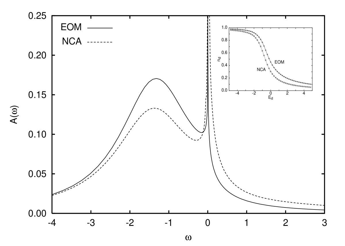
Figure 1: The equilibrium density of states on the quantum dot obtained within $EOM$ (solid line) and $NCA$ (dashed line). Note the relative shift of the spectral weight with respect to the chemical potential $\mu=0$ which results in different occupations shown in the inset. The parameters are: $E_{d}=-2$, $\Gamma_{L}=\Gamma_{R}=1$ and $T=10^{-3}$.

The main features of the $DOS$ remain the same in both approaches. However the height and the width of the Kondo peak is much larger in the $NCA$. Moreover the spectral weight is shifted towards higher energies. In turn this leads to different occupations shown in the inset of the Fig.(1).

Now let’s turn to the nonequilibrium ($\mu_{L}\neq\mu_{R}$) density of states. In this case the high energy features to large extend remain the same as in equilibrium (see Fig.(1)), so the only low energy $DOS$ is shown in the Fig.(2).

Figure 2: The nonequilibrium density of states obtained within $a)$ - $EOM$ and $b)$ - $NCA$ for the symmetric $\Gamma_{L}=\Gamma_{R}$ (solid lines) and asymmetrically coupled quantum dot with $\Gamma_{L}=2\Gamma_{R}$ (dashed) and $\Gamma_{L}=\frac{1}{2}\Gamma_{R}$ (dotted lines). $\mu_{R}=-\mu_{L}=0.2$ and the other parameters are the same as in Fig. (1).

The upper panel presents results obtained via equation of motion technique for Keldysh (matrix) Green’s function.In the lower panel the results obtained with the non-crossing approximation are shown. The coupling is asymmetric with $\Gamma_{L}/\Gamma_{R}=2$ (dashed lines) and $\frac{1}{2}$ (dotted lines). The case of the symmetric coupling $\Gamma_{L}=\Gamma_{R}$ is also shown (solid lines) for comparison. Few features have to be noted. First we see that the Kondo peak is always located at energies coinciding with those of the Fermi levels of the leads. Thus in non-equilibrium we get (in the density of states) two Kondo resonances pinned to Fermi energies of the left and right electrodes. Note also that the heights of the respective Kondo resonances strongly depend on the value of the hybridization. The overall shape of the density of states is similar. The positions of the Kondo peaks are roughly the same but they differ in width and heigths. The peaks obtained in $EOM$, are much narrower and smaller. As a result the curves in figure (2a) differ from that in figure (2b).

These details in the energy dependence of the density of states may shortly be a matter of direct measurements. In fact it has been recently predicted theoretically Lebanon that the on-dot density of states can be measured in a device containing quantum dot coupled to three leads. The very weakly coupled third lead will act as a tunneling tip in conventional tunneling microscope and will probe the non-equilibrium density of states. The conductance spectrum measured by this additional electrode has been shown Lebanon to follow the non equilibrium density of states, like one shown in Fig.(2).

Returning to our main subject we show in Fig.(3) the differential conductance spectrum corresponding to the same ’experimental setup’ as discussed previously in connection with figure (2).

Figure 3: The differential conductance ($G(eV_{SD})=dJ/d(eV_{SD}$)) obtained within $a)$ - $EOM$ and $b)$ - $NCA$ for the symmetric $\Gamma_{L}=\Gamma_{R}$ (solid lines) and asymmetrically coupled quantum dot with $\Gamma_{L}=2\Gamma_{R}$ (dashed) and $\Gamma_{L}=\frac{1}{2}\Gamma_{R}$ (dotted lines).

For comparison we have also plotted in this figure the conductance through the symmetrically coupled quantum dot. In the symmetric situation ($\Gamma_{L}=\Gamma_{R}$) the Kondo resonance is located exactly at zero bias ($V_{DS}=0$), but for $\Gamma_{L}>\Gamma_{R}$ ($\Gamma_{L}<\Gamma_{R}$) it is shifted to the negative (positive) voltages $V_{DS}$. This finding is in nice qualitative agreement with the experimental studies on the transport through the quantum dot in the presence of the asymmetric barriers Simmel . While the observed shifts calculated within $EOM$ and $NCA$ are of comparable magnitude the clear differences in their shape are visible. The $NCA$ peaks are much higher and more symmetric in vicinity of their maxima. For asymmetric coupling the Kondo resonance in the conductance is pinned to the position of the Fermi level of that lead which is more strongly coupled (larger $\Gamma$) to the dot. It is thus mainly the relative coupling which rules the value of the shift.

In Fig.(4) we show the systematic change of the $G(V_{DS})$ with increasing asymmetry $\Gamma_{L}/\Gamma_{R}$ of the coupling.

Figure 4: The differential conductance obtained within $a)$ - $EOM$ and $b)$ - $NCA$ for the different asymmetric couplings. The lower curve is for $\Gamma_{L}=\Gamma_{R}$ while the upper one - $\Gamma_{L}=5.5\Gamma_{R}$. Other parameters are $E_{d}=-10$ and $T=10^{-2}$ in units of $\Gamma_{R}$.

The upper curves in both panels corresponds to $\Gamma_{L}/\Gamma_{R}=5.5$ while lower one is for symmetric coupling $\Gamma_{L}/\Gamma_{R}=1$ in steps of 0.5. The increase of the asymmetry $\Gamma_{L}/\Gamma_{R}$ from $1$ to $5.5$ continuously moves the Kondo peak away from $V_{SD}=0$ position. We have checked that increasing asymmetry to still higher values does not lead to bigger shifts. This is easy to understand as for large asymmetry one of barriers is not transparent enough to produce the clear Kondo resonance in the density of states.

The position of the on-dot electron energy level $E_{d}$ influences anomalous Kondo peak for the asymmetric dot with $\Gamma_{L}/\Gamma_{R}=2$ to lesser extend. It is only important that it takes a value appropriate for observing a Kondo resonance. For all appropriate $E_{d}$ the shifts are of comparable magnitudes.

The data displayed in the figure (4) qualitatively agree with those plotted in figure (5) of vKlitzing and figure (3) of Simmel . However, theoretical shifts of the Kondo peak position are smaller than the experimental.

There may be additional factors which affect the position of the peaks. We have checked that the energy dependence of $\Gamma_{L,R}$ introduces only small quantitative differences in the density of states and differential conductance, and does not lead to better agreement between theory and experiment. Similarly the calculations within $EOM$ approach for finite values of $U$ show that finite $U$ leads to minor corrections as also does the presence of the additional energy levels in the vicinity of Fermi energy. In all the cases studied one gets usual behavior with Kondo peak located at $V_{SD}=0$ for symmetric coupling to both leads and the anomalous Kondo effect for asymmetric coupling. This proves the importance of the asymmetry in the observattion of it.

In experimental setup Simmel the changes of the gate voltage $V_{g}$, which in first place affect the position of the electron energy level also modify the height of the barriers and their transparency $V_{\bf k}$. This effect is of special importance in the quantum dots defined in the two dimensional electron gas where the voltage at a single electrode couples capacitively to other electrodes Buttiker . If we assume that (as in experiments) $\Gamma_{L}/\Gamma_{R}$ remains constant ($=2$) and that the decrease of the energy $E_{d}$ is accompanied by the simultaneous increase of the couplings $\Gamma_{R}$ and $\Gamma_{L}$ then the calculated shifts get larger.

The occurence of the Kondo resonace is possible at low enough temperature. It is also well known non-eq that changes of temperature move slightly the Kondo peak. We have checked this and found that if temperature is raised the position of the peak moves slightly away from the $V_{SD}=0$. At finite temperature the occupation of the dot changes and the Abrikosov-Suhl resonances smear out and this leads to small changes in the position of the Kondo peak.

We thus have combined all above contributions, i.e. assymetry in the couplings $\Gamma_{L}\neq\Gamma_{R}$, their $E_{d}$-dependence, and assumed high enough, but still below $T_{K}$, temperature to get larger shifts of the Kondo peak.

Figure 5: The $NCA$ calculated differential conductance as a function of source-drain voltage $V_{SD}$ for various values of the $E_{d}$ and $\Gamma_{L}$, $\Gamma_{R}$ at fixed $\Gamma_{L}/\Gamma_{R}=2$. The lowest curve correspond to $E_{d}=-3$, $\Gamma_{L}=1$, while upper one is for $E_{d}=-12$, $\Gamma_{L}=6.4$ in units of $\Gamma_{0}$ equal to initial coupling of the left lead. The temperature $T=5\;10^{-2}$ is below estimated Kondo temperatures.

We have shown the results in Fig.(5). The various curves have been calculated for $T=510^{3}$ which is below Kondo temperature. In the figure the change of the position of the on dot energy level is accompanied by the simultaneous change of the barrier transparency. The bottom curve in figure (5)corresponds to $E_{d}=-3\Gamma_{0}$, $\Gamma_{0}=\Gamma_{L}$, while the upper one corresponds to $E_{d}=-12\Gamma_{0}$, $\Gamma_{L}=6.4\Gamma_{0}$. Here $\Gamma_{0}$ is equal to experimentally estimated value of of the smaller of couplings Simmel . The ratio $\Gamma_{R}/\Gamma_{L}$ is kept constant and equal $2$ as estimated in Simmel . The data are in nice qualitative agreement with experiments. The theoretical shifts, however, are smaller than experimental by a factor of $5$-$10$. To check whether this is due to different asymmetry ratio we plot in figure (6) the results obtained for $\Gamma_{R}/\Gamma_{L}=4$. The shifts have increased.

Figure 6: The same as in Fig. (5) but for asymmetry $\Gamma_{L}/\Gamma_{R}=4$. The lowest curve correspond to $E_{d}=-4$, $\Gamma_{L}=1$, while upper one is for $E_{d}=-17.5$, $\Gamma_{L}=12.8$ in units of $\Gamma_{0}$ equal to initial coupling of the left lead.

IV Conclusions

We have found that the emergence of the Kondo peak at non zero voltages $V_{DS}\neq 0$ is caused by asymmetric coupling of the dot to the external electrodes. These results are in qualitative agreement with experimental data on the transport through the quantum dot asymmetrically coupled to the leads vKlitzing ; Simmel . The theoretical Kondo peaks in differential conductance, however, are narrower than experimental ones. Their maxima move to nonzero $V_{SD}$ with increasing the asymmetry or the position of the on-dot energy level. The simultaneous change of $E_{d}$ and $\Gamma_{L}$, $\Gamma_{R}$ can semi-quantitatively explain experimental data. More experimental results are needed to draw firm conclusions such as the applicability of simple Anderson model to asymmetrically coupled quantum dots. It follows from the presented studies that the asymmetry of the couplings is a necessary ingredient for the explanation of the anomalous Kondo effect. Within the Anderson model one always gets normal Kondo effect for symmetric couplings and small shifts of the Kondo peak to non-zero voltages for asymmetric couplings. Our inability to explain quantitatively the experimental data may indicate the necessity of much better theoretical treatment of the model or even better model for the description of these complicated systems. There is a possibility that the experimentally observed features, even though similar to, do not represent genuine Kondo effect. In fact some researches DGG-privat have seen very small shifts, consistent with present calculations, even for quite asymmetrically coupled quantum dots.

Appendix A

To find the current accross the system, Eq.(1), it is enough to calculate the on-dot retarded Green’s function.

The $NCA$ method to get $G^{r}_{\sigma}(\omega)$ has been extensively discussed previously non-eq and there is no need to repeat its derivation again. For the sake of completeness let us only note that we have adapted the formulae derived in the second paper of the reference non-eq .

The $EOM$ method to calculate the $GF$ is straightforward and in $U\rightarrow\infty$ limit leads to

$$G^{r}_{\sigma}(\omega)=\frac{1-\langle n_{-\sigma}\rangle}{\omega-E_{d}-\sum_{\lambda}\Sigma^{r}_{\sigma\lambda}(\omega)}$$ (3)

with the self-energy

$$\Sigma^{r}_{\sigma\lambda}(\omega)=\sum_{\lambda{\bf k}}|V_{\lambda{\bf k}}|^{2}\frac{1+f(\omega-\mu_{\lambda})}{\omega-\epsilon_{\lambda{\bf k}}}.$$ (4)

In the equation (3), $\langle n_{-\sigma}\rangle$ denotes the average on-dot occupation number of the spin $-\sigma$ electrons. In the equilibrium one calculates $\langle n_{-\sigma}\rangle$ self-consistently from the retarded Green’s function $G^{r}_{-\sigma}(\omega)$. Here we are dealing with nonequilibrium situation and $\langle n_{-\sigma}\rangle$ cannot be calculated directly from $G^{r}_{-\sigma}(\omega)$. Instead the nonequilibrium Keldysh Green’s function technique has to be used. The occupation of the dot at time $t$ is expressed via Keldysh ”lesser” Green’s function $\langle n_{\sigma}(t)\rangle=\langle c^{+}_{\sigma}(t)\;c_{\sigma}(t)\rangle=-iG^{<}_{\sigma}(t,t)$. In the steady state one gets

$$\langle n_{\sigma}\rangle=-i\int_{-\infty}^{\infty}\frac{d\omega}{2\pi}G^{<}_{\sigma}(\omega).$$ (5)

This shows that the consistent calculations of the retarded $GF$ requires the knowledge of ”lesser” one. The equation of motion for the ”lesser” $GF$ has been formulated by Niu et al EOM . For the Hamiltonian of the form $H=H_{0}+H_{I}$ they derived the following general equation for the ”lesser” GF

$$\langle\langle A|B\rangle\rangle^{<}_{\omega}=g^{<}(\omega)\langle[A,B]_{\pm}\rangle+g^{r}(\omega)\langle\langle[A,H_{I}]|B\rangle\rangle^{<}_{\omega}+g^{<}(\omega)\langle\langle[A,H_{I}]|B\rangle\rangle^{a}_{\omega},$$ (6)

here $g^{<(r)}(\omega)$ is the ”lesser” (retarded) $GF$ of the noninteracting part $H_{0}$ of Hamiltonian.

To treat strong correlations we use the version MAK-KIW of the slave boson technique and rewrite the Hamiltonian in the form

$$H^{SB}=\sum_{\lambda k\sigma}(\varepsilon_{\lambda k}-\mu_{\lambda})c^{+}_{\lambda k\sigma}c_{\lambda k\sigma}+\varepsilon_{d}\sum_{\sigma}f^{+}_{\sigma}f_{\sigma}+\sum_{\lambda k\sigma}V_{\lambda k}(c^{+}_{\lambda k\sigma}b^{+}f_{\sigma}+f^{+}_{\sigma}bc_{\lambda k\sigma}),$$ (7)

where new fermionic ($f^{+}_{\sigma},f_{\sigma})$ and bosonic ($b^{+},b)$ operators have been introduced. Calculating the on-dot Green’s function $G^{<}_{\sigma}(\omega)=\langle\langle b^{+}f_{\sigma}|f^{+}_{\sigma}b\rangle\rangle^{<}_{\omega}$ we have taken the third term of $H^{SB}$ as an interaction part $H_{I}$ and the first two terms of it as $H_{0}$.

The average occupation number is found to be

$$\langle n\rangle=-\frac{1}{2\pi}\sum_{\sigma}\int^{\infty}_{-\infty}d\omega\;\sum_{\lambda}{\rm Im}\Sigma^{r}_{\sigma\lambda}(\omega)f_{\lambda}(\omega)|G_{\sigma}^{r}(\omega)|^{2}.$$ (8)

Note that in turn it depends on the retarded Green’s function. This closes the system of equations.

References

- (1) T. K. Ng and P. A. Lee, Phys. Rev. 61, 1768 (1989); L. I. Glazman, and M. E. Raikh, Pis’ma Zh. Eksp. Teor. Fiz. 48, 378 (1988) [Engl. transl. JETP] Lett. 47, 452 (1988)]; S. Herschfield, J. H. Davies, and J. W. Wilkins, Phys. Rev. Lett. 67, 3720 (1991); Phys. Rev. bf B46, 7046 (1992).
- (2) Y. Meir N. S. Wingreen, and P. A. Lee, Phys. Rev. Lett. 70, 2601 (1993); N. S. Wingreen, and Y. Meir, Phys. Rev. B49, 11040 (1994); Y. Meir, N. S. Wingreen, P. A. Lee, Phys. Rev. Lett. 66, 3048 (1991).
- (3) D. Goldhaber-Gordon, H. Shtrikman, D. Mahalu, D. Abusch-Magder, U. Meirav, M. A. Kastner, Nature 391, 1569 (1998).
- (4) S. M. Cronenwett, S. M. Maurer, S. R. Pate, C. M. Marens, C. I. Durnöz, J. S. Harris, Jr., Phys. Rev. Lett. 81, 5904 (1998); S. M. Cronenwett, T. H. Oosterkamp, and L. P. Konwenhoven, Science 281, 540 (1998).
- (5) A.C. Hewson The Kondo Problem to Heavy Fermions (Cambridge Universitry Press, Cambridge, UK, 1993); L. Kouwenhoven, L. Glazman, Phys. World, January 2001, p.33.
- (6) D. Goldhbaber-Gordon, J. Göres, M. A. Kastner, H. Shtrikman, D. Mahalu, and U. Meirav, Phys. Rev. Lett. 81, 5225 (1998).
- (7) S. Sasaki, S. De Franceschi, J. M. Elzerman, W. G. van der Wiel, M. Eto, S. Tarucha, L. P. Kouwenhoven, Nature 405, 764 (2000).
- (8) W. G. van der Wiel, S. De Franceschi, T. Fujisawa, J. M. Elzerman, S. Tarucha, L. P. Kouwenhoven, Science 289, 2105 (2000).
- (9) Y. Ji, M. Heiblum, D. Sprinzak, D. Mahalu, H. Shtrikman, Science 290, 779 (2000); Y. Ji, M. Heiblum, H. Shtrikman, Phys. Rev. Lett. 88, 076601 (2002).
- (10) W. G. van der Wiel, S. De Franceschi, J. M. Elzerman, S. Tarucha, L. P. Kouwenhoven, J. Motohisa, F. Nakajima, T. Fukui, Phys. Rev. Lett. 88, 126803 (2002).
- (11) J. Schmid, J. Weis, K. Eberl, K. von Klitzing, Physica B256-258, 182 (1998).
- (12) F. Simmel, R. H. Blick, J. P. Kotthaus, W. Wegscheider, M. Bichler, Phys. Rev. Lett. 83, 804 (1999).
- (13) J.Schmid, J. Weis, K. Eberl, K. v. Klitzing, Phys. Rev. Lett. 84 5824 (2000).
- (14) T. Ivanov, Europhys. Lett. 40, 183 (1997); T. Ivanov, Phys. Rev. B56, 12339 (1997); T. Aono, M. Eto, K. Kawamura, J. Phys. Soc. Jpn. 67, 1860 (1998); R. Aguado, D. C. Langreth, Phys. Rev. Lett. 85, 1946 (2000).
- (15) T. Inoshita, A. Shimizu, Y. Kuramoto, H. Sakaki, Phys. Rev. B48, 14725 (1993); T. Inoshita, Y. Kuramoto, H. Sakaki, Superlatt. and Mictrostr. 22, 75 (1997); T. Pohjola, J. König, M. M. Salomaa, J. Schmid, H. Schoeller, G. Schön, Europhys. Lett. 40, 189 (1997); A. L. Chudnovsky, S. E. Ulloa, Phys. Rev. B63, 165316 (2001); M. Pustilnik, L. I. Glazman, Phys. Rev. Lett. 87, 216601 (2001).
- (16) M. Pustilnik, Y. Avishai, K. Kikoin, Phys. Rev. Lett. 84, 1756 (2000); M. Pustilnik, L. I. Glazman, Phys. Rev. Lett. 85, 2993 (2000); M. Pustilnik, L. I. Glazman, Phys. Rev. B64, 045328 (2001); M. Eto, Y. V. Nazarov, Phys. Rev. Lett. 85, 1306 (2000); M. Eto, Y. V. Nazarov, Phys. Rev. B64, 085322 (2001); D. Giuliano,A. Tagliacozzo, Phys. Rev. Lett. 84, 4677 (2000); D. Giuliano, B. Jouault, A. Tagliacozzo, Phys. Rev. B63, 125318 (2001); W. Hofstetter, H. Schoeller, Phys. Rev. Lett. 88, 016803 (2002).
- (17) L. I. Glazman, F. W. J. Hekking, A. I. Larkin, Phys. Rev. Lett. 83, 1830 (1999); A. Silva, S. Levit, cond-mat/0107595
- (18) Q. Sun, H. Guo, cond-mat/0109145; T. Aono, M. Eto, Phys. Rev. B64, 073307 (2001); V. N. Golovach, D. Loss, cond-mat/0109155.
- (19) A. Kaminski, Y. V. Nazarov, L. I. Glazman, Phys. Rev. B62, 8154 (2000); P. Coleman, C. Hooley, O. Parcollet, Phys. Rev. Lett. 86, 4088 (2001); A. Rosch, J. Kroha, P. Wölfle, Phys. Rev. Lett. 87, 156802 (2001); Y. W. Lee, Y. L. Lee, cond-mat/0105009.
- (20) M. H. Hettler, H. Schoeller, Phys. Rev. Lett. 74, 4907 (1995); T. K. Ng, Phys. Rev. Lett. 76, 487 (1996); Y. Goldin Y. Avishai, Phys. Rev. Lett. 81, 5394 (1998); A. Kaminski, Y. V. Nazarov, L. I. Glazman, Phys. Rev. Lett. 83,384 (1999); P. Nordlander, N. S. Wingreen, Y. Meir, Phys. Rev. B 61, 2146 (2000); M. Plihal, D. C. Langreth, P. Nordlander, Phys. Rev. B61, R13341 (2000); M. Plihal, D. C. Langreth, P. Nordlander, cond-mat/0108525; A. Schiller, S. Hershfield, Phys. Rev. B62, R16271 (2000); R. Lopez, R. Aguado, G. Platero, C. Tejedor, Physica E6, 379 (2000); R. Lopez, R. Aguado, G. Platero, C. Tejedor, Phys. Rev. B64, 075319 (2001); P. Aquado and D.C. Langreth, Phys. Rev. Lett. 85, 1946 (2000).
- (21) L. V. Keldysh, Zh. Eksp. Teor. Fiz. 47, 1515 (1965) [Sov. Phys. JETP 20, 1018 (1965)]; H. Haug, A. P. Jauho, ”Quantum Kinetics in Transport and Optics of Semiconductors”, Springer Verlag, Berlin 1996.
- (22) P. W. Anderson, Phys. Rev. 124, 41 (1961).
- (23) C. Niu, D. L. Lin, T. -H. Lin, J. Phys. Condens. Matt. 11, 1511 (1999).
- (24) M. Krawiec, K. I. Wysokiński, Solid State Commun. 115, 141 (2000).
- (25) Q. Sun, H. Guo, Phys. Rev. B64, 153306 (2001); E. Lebanon, A. Schiller, Phys. Rev. B65, 035308 (2002).
- (26) T. Christen and M. Buttiker, Europhys. Lett. 35, 523 (1996); C.A. Stafford, Phys. Rev. Lett. 77, 2770 (1996).
- (27) D. Goldhaber-Gordon, private communication.