Relaxation Phenomena in Supercomputer Job Arrivals

Abstract

We show that the distribution of supercomputer job submission interarrival times can be understood as a relaxation process. The process of deciding when to submit a job involves a complicated set of interactions between the users themselves, the queuing algorithm, the supercomputer, and a hierarchy of other decision makers. This is analogous to the hierarchically constrained dynamics found in glassy relaxation modelled by a stretched exponential. Empirical supercomputer log data shows that the tails of the distributions are well fit by a stretched exponential.

Today’s supercomputers have thousands of processors and perform sophisticated simulations on a wide variety of problems in material science, structural, and thermal dynamics. Supercomputers are an integral and enabling component in the complex system of Big Science. Among the most powerful supercomputers are those from the Advanced Simulation and Computing Initiative (ASCI)ASC . These machines were built for specific purposes to primarily serve a small group of users who end up dominating the cycles on the machine.

Supercomputers represent the largest single computing resources in the world and they must perform over a staggering range of conditions spanning small interactive jobs to very large jobs, both in terms of the number of processors involved (in the thousands) and for long time periods(on the order of a day or more for a single run). Similar to other complex systems, the workflow of jobs through a supercomputer system is a dynamic and complicated cycle of phases involving submission, dispatch, running, analysis, and resubmission. Often the “output” of a phase depends critically on one or more of the other phases. For example, the submission of a particular job at a particular time by a particular user depends on the time the user has to spend setting up the next run and the previous runs the user has to analyze. These in turn depend upon when it finished running on the machine, which depend upon when it was dispatched, which depend upon the prioritization constraints imposed by the facility managers via the queuing system. On top of these conditions is the laboratory hierarchy who approve projects and above that the governmental funding agencies and finally the elected officials who fund the facilities.

In 1854 Kohlrausch adapted Weber’s famous elasticity equation to explain the residual charge in a Leyden jar as a function of time and discovered the stretched exponential distributionKohlrausch (1854), namely, that the decay time probability of the relaxation process is given by

$$\phi(t)=e^{(-t/\tau)^{\alpha}}.$$ (1)

Since then his equation has found application in numerous relaxation processes of complex systems in nature including colloids, polymers, glasses, and more recently, radio emission from galaxies, earthquakes, oilfield reserve sizes as well as man-made phenomena such as certain market price variations and numbers of citationsLaherrere and Sornette (1998). In this paper we will show how job arrivals at a supercomputer can be mapped to a hierarchical relaxation process and therefore to Kohlrausch’s result.

Heavy-tailed distributions, defined here as those that drop off more slowly than an exponential, including the stretched exponential and power laws, have been reported in a number of manmade phenomena, specifically computer systems. Some examples of heavy tail distributions in computer systems include: computer networks both in terms of their connectivityWillinger et al. (2002) and their traffic patternsWillinger et al. (1996), file systemsGribble et al. (1998), video trafficBeran et al. (1995), software cachesVoldman et al. (1983), and the job size distributions on a single processorHarchol-Barter and Downey (1997). Ultimately, these computer systems are driven by some form of human activity interacting with algorithms hardcoded in the hardware or programmed into the software.

Heavy-tail distributions have important implications for both physical and manmade systems. In particular, heavy tails indicate a significant probability of very large events. In the case of earthquakes it means a meaningful chance for very large and damaging events. In the case of supercomputers it means the possibility that the machine may become overloaded for significant periods of time even if the average turnaround time is moderate. Significantly, the confluence of many large jobs impinging on a supercomputer as a consequence of heavy-tailed distributions both in job size and interarrival time can have serious consequences on the timeliness of the important work done at these facilities. Thus it is important to these facilities that the implications of these heavy-tails be characterized so that they may be taken into account in the design of queuing algorithms and in funding decisions for new hardware.

Despite the work in networks and single processor systems, little is known about the scaling behavior in the largest supercomputers. Given log data from thousands of jobs over a period of several months we can examine these issues quantitatively.

The complicated set of conditions for determining which job gets submitted and when is exactly the sort of conjunctive, i.e., multiplicative, process that is described by the stretched exponential distributionFrisch and Sornette (1997). More specifically, we can think of all the hierarchy of agents interacting in getting a job submitted to be in a discrete set of $N$ pseudospins arrayed in different levels for each agent class. In the case of Big Science the hierarchy is something like user $\rightarrow$ project $\rightarrow$ group $\rightarrow$ facility $\rightarrow$ laboratory $\rightarrow$ government agency $\rightarrow$ executive and legislative entities.

The relaxation function, $\phi$, the probability of the system being in a state at time $t$ is given by

$$\phi(N,t)=1/N\sum_{n=0}^{N}\langle S_{i}(0)S_{i}(t)\rangle$$ (2)

where $S_{i}(t)$ is the state of the $i^{th}$ pseudospin at time $t$ and $N$ is the number of levels. In terms of an ensemble of relaxation times we have

$$\phi(N,t)=\sum_{n=0}^{N}w_{n}\exp(-t/\tau_{n})$$ (3)

where $w_{n}$ is the relative number of pseudospins for level $n$. Following the arguments in Palmer et al. (1984) and Klafter and Shlesinger (1986), only $\mu_{n}\leq N_{n}$ actually contribute to the decision at the $n^{th}$-level of the hierarchy. Under this scenario the $\mu_{n}$ spins in the $n^{th}$-level are free to change only when spins in level $n-1$ have relaxed into one of their $2^{\mu_{n-1}}$ possible states. If we ignore intralevel correlations then

$$\tau_{n+1}=2^{\mu_{n}}\tau_{n}.$$ (4)

Defining $\tilde{\mu}_{k}=\mu_{k}\ln 2$ then

$$\tau_{n+1}=\tau_{0}\exp\left(\sum_{k=0}^{n}\tilde{\mu}_{k}\right).$$ (5)

For a glassy relaxation, $\mu_{n}$ should decrease rapidly enough to make Eq.(5) converge. One such condition is given by $\mu_{n}=\mu_{0}/n$. For the job submission hierarchy we are considering, $\mu_{0}$ is about $100-1000sec$, the average time between job submissions, the next level might be weekly meetings, a factor of ten thousand. For the highest levels in the hierarchy, the decisions are made on a much compressed scale relative to the next highest level. For example, the penultimate level meets quarterly and the highest level on a yearly scale, a difference of only a factor of $4$.

We also need to model the branching ratio between levels, or “span of control” in bureaucracy parlance. We model this as

$$w_{n}=w_{0}\lambda^{-n}.$$ (6)

Converting the sum to an integral we have

$$\phi(t)=w_{0}\int_{0}^{\infty}\lambda^{-n}\exp(-tn^{-\tilde{\mu}_{0}}/\tau_{0})dn$$ (7)

This equation cannot be solved in closed form so by the method of steepest descent expanding around the point $n\propto t^{\alpha}$ we finally obtain the desired result, Eq.(1), where $\tau$ defines a characteristic scale to the distribution (contrast this with a power law’s scale free behavior) and finally

$$\alpha=1/(1+\tilde{\mu}_{0})$$ (8)

is a measure of the heaviness of the tail. The smaller the value of $\alpha$, the heavier the tail.

Another way of looking at a relaxation process is as a random walk in a fractal spaceJund et al. (2001). When the relaxation process is described by a stretched exponential this is seen as the signature of a fractal morphology of the configuration space at the current temperature of the system. In this view the complex morphology of the job submission landscape as the set of necessary steps needed for submission fall into place is what drives the system into its heavy-tailed relaxation. Table 1 shows an analogy between job events and a spin relaxation process.

Table 1: Job event analogy to a spin relaxation process in Nature.

Process	Spin Glass	Job interarrival time
Energy Source	Heat	Project deliverables
Energy Storage	Spins	Pending work
Threshold	Glass transition	Job preparation
	temperature
Energy Release	Glass transition	Job submission

To demonstrate that supercomputer job submissions can be understood as a stretched exponential relaxation process, we analyzed job logs from the ASCI supercomputers ASCI-BlueMountain (Los Alamos National Laboratory), and ASCI-BluePacific (Lawrence Livermore National Laboratory)ASC . Each lab has devised its own method for queuing jobs based in part on the historical political realities at each labClearwater and Kleban (2002a). The important thing to keep in mind is that the queuing algorithm through its prioritization and “backfilling,” (running jobs that are not first in the queue but can run now without slowing down the first job in the queue) acts to alter the order that jobs were submitted and thus when they will be dispatched, run, and finally analyzed, all affecting the next job to be submitted and thus the interarrival submission times.

For all the analysis shown below we tried to fit other distributions such as the exponential, lognormal, and power law functions, but none provided as good a fit and over such a long range as the stretched exponential. Qualitatively, the exponential fell off more rapidly than the data and the power law not fast enough. The lognormal fit well for smaller values, but did poorly at larger values, as one would expect from its functional form. Intuitively, we might expect the stretched exponential to be applicable and fill in this intermediate range with a moderately heavy tail and a characteristic scale.

Blue Mountain at Los Alamos has 5418 processors in its large partition.There were 8171 jobs in this sample taken over a period of 83 days. The distribution of interarrival times is shown in Fig. 1. The best fit (short dashes) to a stretched exponential is shown with a characteristic time of $\tau=524$s and $\alpha=.57$. Fits to lognormal and exponential are also shown. As can clearly be seen, only the stretched exponential is able to model the data well over its entire range.

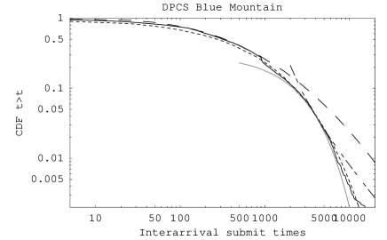
Figure 1: The cumulative distribution function for the time between job submissions. The average is 879s and the maximum is 161,311s. The solid curve is the data, the dashed are from a stretched exponential fit. The long dashed curve is a best fit to a lognormal, the gray curve is the best fit to an exponential, and the dot-dash is a power law over a restricted region.

The results from Blue Pacific at Livermore consisted of 57,430 jobs taken over a period of 63 days. Unlike Blue Mountain, Blue Pacific did not have any partitions and used about 1000 CPUs, although the full machine has more. The part of Blue Pacific we used was no longer fulfilling its primary mission to the ASCI program and is involved in more academic research.

Fig. 2 shows the cumulative distribution function for interarrival times. We have truncated our fit at 10,000 seconds because beyond that time the interarrival times are likely due to system issues and not user issues. For example, these events may correspond to outages in the machine or logging errors(about 10% of the log had bogus entries and were not used) that could anomalously effect the very long portion of the tail. For interarrival times up to 10,000s the parameters for the stretched exponential are a characteristic time of $\tau=1655$s and $\alpha=0.61$.

Figure 2: The cumulative distribution function for the interarrival time between job submissions. The solid curve is the log data, the dashed curve is the fitted stretched exponential.

The parameters we found for the stretched exponential fit are shown in Table 2. It is interesting to note that for the interarrival time distribution, both LSF and DPCS have similar exponents for large jobs, $\alpha_{LSF}=0.57$ and $\alpha_{DPCS}=0.61$.

Table 2: Stretched exponential parameters for LSF and DPCS data.

	Interarrival time
	$\tau$sec	$\alpha$
LSF	$524$	$0.57$
DPCS	$1655$	$0.61$

Our results have shown the applicability for the first time of the stretched exponential to describing distributions from supercomputer systems. Remarkably, the stretched exponential provided a good fit over the entire range of values for some of the cases we studied, spanning up to 8 orders of magnitude.

One interesting implication of the constrained hierarchical model we are using is the relationship between levels in the hierarchy, Eq.(4), which implies that relaxation (or response times in our case) take much longer as one gets farther from those doing the actual work. Interpreting the job submission process as a relaxation phenomenon where “barriers” to the decision to submit a certain sized job at a certain time must be overcome, the exponent $\alpha$ may be understood as related to the number of levels in a hierarchy that underlies the overall job submission processFrisch and Sornette (1997); Laherrere and Sornette (1998); Palmer et al. (1984).

We can test the convergence of 3 by using parameters derived from the supercomputers. Using the empirically determined value of $\alpha_{LSF}=0.57$, so that $\tilde{\mu}_{0}=0.75$ from Eq.(8). Values of $\mu_{n}<1$ correspond to weak constraints between levelsPalmer et al. (1984), not surprising in a scientific environment. Since we are plotting cumulative distribution functions, the $w_{n}$’s themselves don’t matter, but the span of control is critical. We choose $\lambda=5$ which is a typical span of control, $\lambda$ Eq. (7), in a high tech research lab. For $\tau_{0}$ we use the average time between job submissions, $787$s. We then plot $\phi(N,t)$ for $N=1$ to $4$ in Fig. 3. The sum converges quickly and approximates that of the exact stretched exponential. From an organizational standpoint this tells us that no more than 4 or so levels in the hierarchy are having any effect on the time scale at which work gets done.

Figure 3: The cumulative distribution function for the interarrival time between job submissions using the fitted values(heavy curve) and the first $\phi(N,t)$ for $N=1$ to $4$.

Both the supercomputers utilized in this research run under a “Fair Share”Henry (1984); Kay and Lauder (1988) algorithm (user priorities are decreased if they go over their “share”) so it will be interesting to see, when data becomes available, if another queuing algorithm, such as NQS (essentially first-in first-out) at Sandia has a similar characteristic exponent for job sizes and job interarrival times.

The characteristic scale implied by the stretched exponential distribution may prompt another look at some computer phenomena previously thought to exhibit scale-free behavior. It also tells us that the deviations from a power law are a fundamental part of the phenomenaLaherrere and Sornette (1998). After all, as big as these supercomputers are, they are still finite and their operators have put in additional constraints as well to satisfy administrative requirements, i.e., political realities. Together these constraints act to define a characteristic size of the distribution as well as the heaviness of the tail. For example, the size of jobs measured in terms of number of processors and run time was also found to be well modelled by a stretched exponential.Clearwater and Kleban (2002b)

In conclusion, we have shown that the interarrival time of jobs are not exponential nor do they posses pure power-law tails, but are somewhere in between and can be well fit by stretched exponentials over a large and important part of their range. These are indicative of finite scaling behaviors and have implications for the ultimate performance of these facilities because they relate to the frequency, and therefore the turnaround of big jobs that are the bread and butter of the ASCI supercomputers.

This paper would not have been possible with the expertise of many people who provided us with detailed knowledge of algorithms, data formats, as well as providing the job log data. The authors gratefully acknowledge the assistance of Stephany Boucher, Charles Hales, Michael Hannah, Steve Humphreys, Moe Jette, Wilbur Johnson, Tom Klingner, Jerry Melendez, Amy Pezzoni, Randall Rheinheimer, Phil Salazar, Bob Wood, and Andy Yoo. Sandia is a multiprogram laboratory operated by Sandia Corporation, a Lockheed Martin Company, for the United States Department of Energy under Contract DE-AC04-94AL85000.

References

- (1) eprint http://www.llnl.gov/asci/.
- Kohlrausch (1854) R. Kohlrausch, Pogg. Ann. Phys. Chem. 91, 179 (1854).
- Laherrere and Sornette (1998) J. Laherrere and D. Sornette, European Physics Journal B 2, 525 (1998).
- Willinger et al. (2002) W. Willinger, R. Govindan, S. Jamin, V. Paxson, and S. Shenker, Proceedings of the National Academy of Sciences 99, 2573 (2002).
- Willinger et al. (1996) W. Willinger, M. Taqqu, and A. Erramilli (1996).
- Gribble et al. (1998) S. D. Gribble, G. S. Manku, D. S. Roselli, E. A. Brewer, T. J. Gibson, and E. L. Miller, in Measurement and Modeling of Computer Systems (1998), pp. 141–150, URL citeseer.nj.nec.com/236792.html.
- Beran et al. (1995) J. Beran, R. Sherman, M. S. Taquu, and W. Willinger, IEEE Transactions on Communications 43 (1995).
- Voldman et al. (1983) J. Voldman, B. Mandelbrot, L. Hoevel, and P. R. J. Knight, IBM Journal of Research and Development 27, 164 (1983).
- Harchol-Barter and Downey (1997) M. Harchol-Barter and A. Downey, ACM Transactions in Computer Systems 15 (1997).
- Frisch and Sornette (1997) U. Frisch and D. Sornette, Phys. I France 7 (1997).
- Palmer et al. (1984) R. G. Palmer, D. L. Stein, E. Abrahams, and P. W. Anderson, Phys. Rev. Lett. pp. 958–961 (1984).
- Klafter and Shlesinger (1986) J. Klafter and M. F. Shlesinger, Proc. Nat. Acad. Sci. 83, 848 (1986).
- Jund et al. (2001) P. Jund, R. Julien, and I. Campbell, Phys. Rev. E 63, 036131 (2001).
- Clearwater and Kleban (2002a) S. H. Clearwater and S. D. Kleban, in 16th International Parallel & Distributed Processing Symposium (2002a).
- Henry (1984) G. J. Henry, AT&T Bell Lab. Tech. Journal 63, 1845 (1984).
- Kay and Lauder (1988) J. Kay and P. Lauder, Comm. of the ACM 31, 44 (1988).
- Clearwater and Kleban (2002b) S. H. Clearwater and S. D. Kleban, Tech. Rep. SAND2002-2378C, Sandia National Laboratories (2002b).