Exact integral equation for the renormalized Fermi surface

Abstract

The true Fermi surface of a fermionic many-body system can be viewed as a fixed point manifold of the renormalization group (RG). Within the framework of the exact functional RG we show that the fixed point condition implies an exact integral equation for the counterterm which is needed for a self-consistent calculation of the Fermi surface. In the simplest approximation, our integral equation reduces to the self-consistent Hartree-Fock equation for the counterterm.

In his authoritative book on interacting Fermi systems Nozières wrote fourty years ago Nozieres64 : “In practice, we shall never try to calculate the Fermi surface, which is much too difficult.” What is the reason for this difficulty? Formally, the Fermi surface of an interacting Fermi system is defined as the set of all wavevectors ${\bf{k}}_{F}$ satisfying Luttinger60

$$\epsilon_{{\bf{k}}_{F}}-\mu+\Sigma({\bf{k}}_{F},i0)=0\;,$$ (1)

where $\epsilon_{\bf{k}}$ is the energy dispersion in the absence of interactions, $\mu$ is the chemical potential, and $\Sigma({\bf{k}},\omega)$ is the exact self-energy of the interacting system footnotereal . For simplicity we assume an infinite and spin-rotationally invariant system at zero temperature, so that $\Sigma({\bf{k}},\omega)$ is independent of the spin. Unfortunately, the function $\Sigma({\bf{k}}_{F},i0)$ in Eq. (1) is not known a priori, so that the calculation of the true Fermi surface requires the solution of the many-body problem.

For weak interactions, one might try to determine the Fermi surface perturbatively by simply calculating $\Sigma({\bf{k}},i0)$ in powers of the interaction and substituting the result into Eq. (1). However, in general the perturbation series contains anomalous terms Kohn60 with unphysical singularities, which are generated because the ground state of the non-interacting system evolves into an excited state of the interacting system when the interaction is adiabatically switched on. As discussed by Nozières Nozieres64 , this artificial level crossing can be avoided by introducing counterterms which are determined by the requirement that the Fermi surface remains fixed as the interaction is adiabatically switched on. This intuitive idea can be implemented perturbatively as follows Nozieres64 ; Feldman96 : Suppose we would like to know the true Fermi surface of a system with Hamiltonian ${H}={H}_{0}+{H}_{1}$, where ${H}_{1}$ describes some general two-body interaction and the non-interacting part is given by

$${H}_{0}=\sum_{{\bf{k}},\sigma}\epsilon_{\bf{k}}c^{\dagger}_{{\bf{k}}\sigma}c_{{\bf{k}}\sigma}\;.$$ (2)

Here $c_{{\bf{k}}\sigma}$ are the usual annihilation operators of fermions with momentum ${\bf{k}}$ and spin $\sigma$. An expansion in powers of $H_{1}$ leads to Feynman diagrams where vertices corresponding to $H_{1}$ are connected by propagators $G_{0}({\bf{k}},\omega)=[\omega-\epsilon_{\bf{k}}+\mu]^{-1}$. These are singular for $\omega=0$ and $\epsilon_{\bf{k}}=\mu$, which is not the true Fermi surface defined in Eq. (1). If the perturbative expansion is truncated at a finite order, this leads to the unphysical divergencies mentioned above Kohn60 . To avoid these, we add the counterterm $\sum_{{\bf{k}}\sigma}\Sigma({\bf{k}}_{F},i0)c^{\dagger}_{{\bf{k}}\sigma}c_{{\bf{k}}\sigma}$ to $H_{0}$ and subtract it again from $H_{1}$, writing $H=H_{0}^{\prime}+H_{1}^{\prime}$, with

$${H}_{0}^{\prime}=\sum_{{\bf{k}}\sigma}[\epsilon_{\bf{k}}+\Sigma({\bf{k}}_{F},i0)]c^{\dagger}_{{\bf{k}}\sigma}c_{{\bf{k}}\sigma}\;,$$ (3)

and $H_{1}^{\prime}=H_{1}-\sum_{{\bf{k}}\sigma}\Sigma({\bf{k}}_{F},i0)c^{\dagger}_{{\bf{k}}\sigma}c_{{\bf{k}}\sigma}$. Here ${\bf{k}}_{F}$ is the wavevector closest to ${\bf{k}}$ lying on the Fermi surface, see Fig. 1.

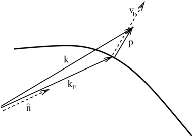
Figure 1: Decomposition ${\bf{k}}=\hat{\bf{n}}k_{F}(\hat{\bf{n}})+{\bf{p}}$ of a wavevector ${\bf{k}}$ into a component ${\bf{k}}_{F}=\hat{\bf{n}}k_{F}(\hat{\bf{n}})$ on the Fermi surface and a component ${\bf{p}}$ in the direction of the local Fermi velocity ${\bf{v}}_{F}$. The thick solid line is a part of the Fermi surface. This construction defines ${\bf{k}}_{F}$ and $\hat{\bf{n}}$ as a function of ${\bf{k}}$. Here ${\bf{v}}_{F}=\nabla_{{\bf{k}}}\epsilon_{{\bf{k}}}|_{{\bf{k}}={\bf{k}}_{F}}$ is defined in terms of the gradient of the free dispersion at the true Fermi surface, so that ${\bf{v}}_{F}$ is not necessarily perpendicular to the Fermi surface.

Using Eq. (1), the corresponding free propagator can then be written as $G_{0}^{\prime}({\bf{k}},\omega)=[\omega-\epsilon_{\bf{k}}+\epsilon_{{\bf{k}}_{F}}]^{-1}$, which by construction is singular on the true Fermi surface. But how do we find the counterterm necessary to calculate $\epsilon_{{\bf{k}}_{F}}$? Following the usual strategy adopted in field theory ZinnJustin89 , we may expand the irreducible self-energy associated with the modified interaction $H_{1}^{\prime}$ perturbatively in powers of $H_{1}^{\prime}$ and require that, order by order in perturbation theory, the corrections vanish when we set $\omega=0$ and ${\bf{k}}={\bf{k}}_{F}$. This renormalized perturbation theory leads to complicated integral equations for $\Sigma({\bf{k}}_{F},i0)$, which must be solved numerically Neumayr02 .

A few years ago Anderson Anderson93 critically discussed a simplified version of the renormalized perturbation theory outlined above, where $\Sigma({\bf{k}}_{F},i0)$ is replaced by a constant $\delta\mu$. He correctly pointed out that in general it is not allowed to ignore the momentum-dependence of the counterterms, and argued that in two dimensions the effective interaction between electrons with opposite spin and wavevectors on the true Fermi surface depends in a subtle way on the boundary conditions which cannot be adequately taken into account perturbatively. To gain a better understanding of this problem, it should be useful to have an algorithm for calculating the Fermi surface which does not rely on the perturbative expansion of counterterms in powers of the interaction. In this work we show that such an algorithm follows in a straightforward way from the exact functional renormalization group (RG) approach described in Ref.Kopietz01 .

In the past decade several authors have used Wilsonian RG methods to study interacting Fermi systems Kopietz01 ; Benfatto90 ; Polchinski92 ; Shankar94 ; Zanchi96 ; Salmhofer98 ; Halboth00 ; Binz02 , using different versions of the RG. In particular, the RG transformations used in Refs. Zanchi96 ; Salmhofer98 ; Halboth00 ; Binz02 exclusively focus on the mode elimination step. Although such a procedure is sufficient if one considers only the one-loop flow of marginal couplings, in general a complete Wilsonian RG transformation consists not only of the mode elimination, but includes also the rescaling of momenta, frequencies and fields Ma76 . While the field rescaling (i.e. the wavefunction renormalization) becomes only important beyond the one-loop approximation, the RG flow of all relevant and irrelevant couplings is determined in an essential way by the rescaling step even at the one-loop level. We emphasize that the rescaling of momenta and frequencies is more than a trivial mathematical change of variables – it is crucial to detect possible fixed points of the RG and to calculate critical exponents Ma76 . Moreover, as will be shown below, the length and time rescaling is very helpful for a derivation of the self-consistent Hartree-Fock approximation within the framework of the exact RG. The importance of rescaling in the presence of a Fermi surface has been emphasized by Polchinski Polchinski92 and by Shankar Shankar94 . In Ref.Kopietz01 we have shown how the exact functional RG approach developed previously Zanchi96 ; Salmhofer98 ; Halboth00 can be modified to include the rescaling step. Here, we shall show that the rescaling is crucial to obtain a non-perturbative definition of the Fermi surface as a fixed point manifold of the RG. We obtain an explicit algorithm for calculating the Fermi surface which does not rely on the iterative procedure of fixing the counterterms order by order in perturbation theory. The fixed point property of the Fermi surface has also been emphasized by Ferraz Ferraz02 , who recently discussed the Fermi surface renormalization in a special two-dimensional system using the field theoretical RG.

The exact functional RG can be formulated in terms of an infinite hierarchy of coupled differential equations for the irreducible $2n$-point vertices $\Gamma^{(2n)}_{\xi}(K_{1}^{\prime},\ldots,K_{n}^{\prime};K_{n},\ldots,K_{1})$, where $K=(\sigma,{\bf{k}},i\omega)$ is a collective label for spin projection $\sigma$, momentum ${\bf{k}}$, Matsubara frequency $i\omega$. Here $\xi$ is an infrared cutoff with units of energy which regularizes the singularity of the free propagator. To scale wavevectors toward the Fermi surface, it is convenient to perform a non-linear coordinate transformation in momentum space, ${\bf{k}}=\hat{\bf{n}}k_{F}(\hat{\bf{n}})+\hat{\bf{v}}_{F}\xi q/|{\bf{v}}_{F}|$, and eliminate ${\bf{k}}$ in favor of the dimensionless variable $q$ and the unit vector $\hat{\bf{n}}$. Here $k_{F}(\hat{\bf{n}})$ is the length of ${\bf{k}}_{F}$ parameterized by $\hat{\bf{n}}$, and ${\bf{v}}_{F}=\nabla_{\bf{k}}\epsilon_{\bf{k}}|_{{\bf{k}}_{F}}$ is the Fermi velocity of the non-interacting system at the true ${\bf{k}}_{F}$, see Fig. 1. The corresponding unit vector is denoted by $\hat{\bf{v}}_{F}={\bf{v}}_{F}/|{\bf{v}}_{F}|$. Geometrically, $q={\bf{v}}_{F}\cdot{\bf{p}}/\xi={\bf{v}}_{F}\cdot({\bf{k}}-\hat{\bf{n}}k_{F}(\hat{\bf{n}}))/\xi$ measures the distance of a given ${\bf{k}}$ from the Fermi surface in units of the infrared cutoff. We also define rescaled frequencies $\epsilon=\omega/\xi$, and label the degrees of freedom by $Q=(\sigma,\hat{\bf{n}},q,i\epsilon)$ instead of $K$. To implement the scaling toward the Fermi surface Polchinski92 we consider the RG flow of the following rescaled vertices Kopietz01

$$\tilde{\Gamma}_{t}^{(2n)}(Q_{1}^{\prime},\ldots,Q_{n}^{\prime};Q_{n},\ldots,Q_{1})=$$ (4)

$$\nu_{0}^{n-1}\xi^{n-2}\left[Z_{t}^{\hat{\bf{n}}_{1}^{\prime}}\cdots Z_{t}^{\hat{\bf{n}}_{n}^{\prime}}Z_{t}^{\hat{\bf{n}}_{n}}\cdots Z_{t}^{\hat{\bf{n}}_{1}}\right]^{1/2}$$

$$\times\Gamma^{(2n)}_{\xi}(K_{1}^{\prime},\ldots,K_{n}^{\prime};K_{n},\ldots,K_{1})\;.$$

Here $t=-\ln(\xi/\xi_{0})$ is a logarithmic flow parameter, $\nu_{0}=\int\frac{d{\bf{k}}}{(2\pi)^{D}}\delta(\epsilon_{{\bf{k}}}-\epsilon_{{\bf{k}}_{F}})$ is the density of states (per spin projection) of the non-interacting system at the true Fermi surface, and

$$Z_{t}^{\hat{\bf{n}}}=\left[1-\left.\frac{\partial\Sigma_{\xi}({\bf{k}}_{F},\omega+i0)}{\partial\omega}\right|_{\omega=0}\right]^{-1}$$ (5)

is the wavefunction renormalization factor, where $\Sigma_{\xi}({\bf{k}},i\omega)$ is the irreducible self-energy of the system with infrared cutoff $\xi=\xi_{0}e^{-t}$. To determine the true Fermi surface self-consistently it turns out to be useful to subtract the counterterm $\Sigma({\bf{k}}_{F},i0)$ from the irreducible two-point vertexKopietz01 , defining

$$\tilde{\Gamma}_{t}^{(2)}(Q)=\frac{Z_{t}^{\hat{\bf{n}}}}{\xi}\Gamma^{(2)}_{\xi}(K)=-\frac{Z_{t}^{\hat{\bf{n}}}}{\xi}\left[\Sigma_{\xi}(K)-\Sigma({\bf{k}}_{F},i0)\right]\;.$$ (6)

The subtracted two-point vertex satisfies the exact flow equation Kopietz01

$$\partial_{t}\tilde{\Gamma}_{t}^{(2)}(Q) = (1-\eta_{t}^{\hat{\bf{n}}}-q\partial_{q}-\epsilon\partial_{\epsilon})\tilde{\Gamma}_{t}^{(2)}(Q)$$ (7)

$$- \int_{Q^{\prime}}\dot{G}_{t}(Q^{\prime})\tilde{\Gamma}_{t}^{(4)}(Q,Q^{\prime};Q^{\prime},Q)\;,$$

where $\eta_{t}^{\hat{\bf{n}}}=-\partial_{t}\ln Z_{t}^{\hat{\bf{n}}}$ is the flowing anomalous dimension (which vanishes for large $t$ if the system is a Fermi liquid). The integration measure in Eq. (7) is defined by

$$\int_{Q}=\sum_{\sigma}\int\frac{dS_{\hat{\bf{n}}}}{S_{D}}\int dqJ({\hat{\bf{n}}},q)\int\frac{d\epsilon}{2\pi}\;\;,$$ (8)

where $dS_{\hat{\bf{n}}}$ is a surface element and $S_{D}$ is the surface area of the unit sphere in $D$ dimensions, and $J({\hat{\bf{n}}},q)$ is the Jacobian associated with the transformation ${\bf{k}}\rightarrow(\hat{\bf{n}},q)$ divided by $\nu_{0}\xi^{2}$. The function $\dot{{G}}_{t}(Q)$ in Eq. (7) is defined by

$$\dot{{G}}_{t}(Q)=\frac{\delta(\tilde{\Omega}_{Q}-1)}{Z_{t}^{\hat{\bf{n}}}\left[i\epsilon-\xi_{t}^{\hat{\bf{n}}}(q)\right]+\tilde{\Gamma}_{t}^{(2)}(Q)}\;,$$ (9)

where $\xi_{t}^{\hat{\bf{n}}}(q)=(\epsilon_{{\bf{k}}_{t}}-\epsilon_{{\bf{k}}_{F}})/{\xi}$, with ${\bf{k}}_{t}=\hat{\bf{n}}k_{F}(\hat{\bf{n}})+\hat{\bf{v}}_{F}\xi_{0}e^{-t}q/|{\bf{v}}_{F}|$. Here $\tilde{\Omega}_{Q}$ is some function that measures the distance from the Fermi surface, for example $\tilde{\Omega}_{Q}=|\xi_{t}^{\hat{\bf{n}}}(q)|\approx|q|$. The flow equation of the rescaled irreducible four-point vertex $\tilde{\Gamma}_{t}^{(4)}(Q_{1}^{\prime},Q_{2}^{\prime};Q_{2},Q_{1})$ is not explicitly needed in this work; it can be found in Ref.Kopietz01 .

The shape of the Fermi surface of the interacting system is determined by the RG flow of the couplings

$$\tilde{\mu}_{t}^{\hat{\bf{n}}}\equiv\tilde{\Gamma}_{t}^{(2)}(\sigma,\hat{\bf{n}},q=0,i\epsilon=i0)\;.$$ (10)

From Eq. (7) we see that these couplings satisfy the exact flow equation

$$\partial_{t}\tilde{\mu}_{t}^{\hat{\bf{n}}}=(1-\eta_{t}^{\hat{\bf{n}}})\tilde{\mu}_{t}^{\hat{\bf{n}}}+\dot{\Gamma}_{t}^{(2)}(\hat{\bf{n}})\;,$$ (11)

with

$$\dot{\Gamma}_{t}^{(2)}(\hat{\bf{n}})=-\int_{Q^{\prime}}\dot{G}_{t}(Q^{\prime})\tilde{\Gamma}_{t}^{(4)}(Q_{0},Q^{\prime};Q^{\prime},Q_{0})\;,$$ (12)

where $Q_{0}=(\sigma,\hat{\bf{n}},q=0,i\epsilon=i0)$. Note that in dimensions $D>1$ there are infinitely many couplings $\tilde{\mu}_{t}^{\hat{\bf{n}}}$, labelled by the unit vector $\hat{\bf{n}}$. Obviously, each $\tilde{\mu}_{t}^{\hat{\bf{n}}}$ with $\eta_{\infty}^{\hat{\bf{n}}}=\lim_{t\rightarrow\infty}\eta_{t}^{\hat{\bf{n}}}<1$ is relevant, so that some fine tuning of the bare couplings $\tilde{\mu}_{0}^{\hat{\bf{n}}}$ is necessary to force $\tilde{\mu}_{t}^{\hat{\bf{n}}}$ to flow into a fixed point of the RG. Because a finite limit $\tilde{\mu}_{\infty}^{\hat{\bf{n}}}=\lim_{t\rightarrow\infty}\tilde{\mu}_{t}^{\hat{\bf{n}}}$ means that we have found the true Fermi surface of the interacting system Kopietz01 , we conclude that the detailed shape of the Fermi surface is sensitive to the numerical values of the bare couplings of the theory. Polchinski Polchinski92 pointed out that such a fine tuning of the bare couplings is unnatural, because physical effects which depend on the precise shape of the Fermi surface are not protected against small perturbations.

To further elucidate the relation between the relevant couplings $\tilde{\mu}_{t}^{\hat{\bf{n}}}$ and the shape of the Fermi surface, let us explicitly derive from Eq. (11) a self-consistency condition for the Fermi surface. Therefore it is useful to transform Eq. (11) into an integral equation,

$$\tilde{\mu}_{t}^{\hat{\bf{n}}}=e^{t-\int_{0}^{t}d\tau\eta_{\tau}^{\hat{\bf{n}}}}\left[\tilde{\mu}_{0}^{\hat{\bf{n}}}+\int_{0}^{t}dt^{\prime}e^{-t^{\prime}+\int_{0}^{t^{\prime}}d\tau\eta_{\tau}^{\hat{\bf{n}}}}\dot{\Gamma}^{(2)}_{t^{\prime}}(\hat{\bf{n}})\right]\;.$$ (13)

Suppose now that we have adjusted the bare couplings such that for $t\rightarrow\infty$ the flowing couplings $\tilde{\mu}_{t}^{\hat{\bf{n}}}$ indeed approach finite fixed point values. Assuming that the associated anomalous dimensions $\eta_{\infty}^{\hat{\bf{n}}}$ are smaller than unityfootnoteeta , we conclude from Eq. (13) that the limit $\tilde{\mu}_{\infty}^{\hat{\bf{n}}}=\lim_{t\rightarrow\infty}\tilde{\mu}_{t}^{\hat{\bf{n}}}$ can only be finite if the initial values $\tilde{\mu}_{0}^{\hat{\bf{n}}}$ are chosen such that

$$\tilde{\mu}_{0}^{\hat{\bf{n}}} = -\int_{0}^{\infty}dte^{-t+\int_{0}^{t}d\tau\eta_{\tau}^{\hat{\bf{n}}}}\dot{\Gamma}^{(2)}_{t}(\hat{\bf{n}})$$

$$= \int_{0}^{\infty}dte^{-t+\int_{0}^{t}d\tau\eta_{\tau}^{\hat{\bf{n}}}}\int_{Q^{\prime}}\dot{G}_{t}(Q^{\prime})\tilde{\Gamma}_{t}^{(4)}(Q_{0},Q^{\prime};Q^{\prime},Q_{0})\;.$$

This is an implicit equation for $\tilde{\mu}_{0}^{\hat{\bf{n}}}$, relating it to the values of the two-point vertex and the four-point vertex on the entire RG trajectory. Keeping in mind that the right-hand side of Eq. (LABEL:eq:integral2) implicitly depends on $\tilde{\mu}^{{\hat{\bf{n}}}}_{t}$ and that according to Eq. (6)

$$\Sigma({\bf{k}}_{F},i0)-\Sigma_{\xi_{0}}({\bf{k}}_{F},i0)=\xi_{0}\tilde{\mu}_{0}^{\hat{\bf{n}}}/Z_{0}^{\hat{\bf{n}}}\;,$$ (15)

it is obvious that Eq. (LABEL:eq:integral2) can be regarded as an integral equation for the counterterm $\Sigma({\bf{k}}_{F},i0)$, the solution of which yields the true shape of the Fermi surface. At this point it is instructive to transform Eq. (LABEL:eq:integral2) back to unrescaled variables, choosing for simplicity the initial conditions $\Sigma_{\xi_{0}}({\bf{k}}_{F},i0)=0$ and $Z_{0}^{\hat{\bf{n}}}=1$. Using the above definitions we find that Eq. (LABEL:eq:integral2) is equivalent with

$$\Sigma({\bf{k}}_{F},i0) = \sum_{\sigma^{\prime}}\int\frac{d{\bf{k}}^{\prime}}{(2\pi)^{D}}\frac{d\omega^{\prime}}{2\pi}\frac{\Theta(\xi_{0}-\xi_{{\bf{k}}^{\prime}})}{i\omega^{\prime}-\epsilon_{{\bf{k}}^{\prime}}+\mu-\Sigma_{\xi_{{\bf{k}}^{\prime}}}(K^{\prime})}$$ (16)

$$\times\Gamma^{(4)}_{\xi_{{\bf{k}}^{\prime}}}({\bf{k}}_{F},i0,\sigma,{\bf{k}}^{\prime},i\omega^{\prime},\sigma^{\prime};{\bf{k}}^{\prime},i\omega^{\prime},\sigma^{\prime},{\bf{k}}_{F},i0,\sigma)\;,$$

where $\xi_{{\bf{k}}^{\prime}}=|\epsilon_{{\bf{k}}^{\prime}}-\epsilon_{{\bf{k}}_{F}^{\prime}}|$. Note that the right-hand side of Eq. (16) involves the flowing self-energy and four-point vertex at the scales $\xi=\xi_{{\bf{k}}^{\prime}}$ which depend on the distance from the true Fermi surface. We emphasize that the exact integral equation (16) and the equivalent rescaled equation (LABEL:eq:integral2) fix the counterterm $\Sigma({\bf{k}}_{F},i0)$ from the requirement that for $t\rightarrow\infty$ all couplings approach finite fixed point values.

If the system is a Luttinger liquid, then the rescaled version (LABEL:eq:integral2) of the self-consistency equation is more convenient than the unrescaled version (16), because for a Luttinger liquid the marginal part of the four-point vertex vertex $\Gamma^{(4)}_{\xi}$ without wavefunction renormalization factors diverges for $\xi\rightarrow 0$, while the rescaled four-point vertex $\tilde{\Gamma}^{(4)}_{t}$ defined in Eq.(4) approaches for $t\rightarrow\infty$ a finite limit. In this case the divergence of the unrescaled $\Gamma^{(4)}_{\xi}$ is canceled by the vanishing wavefunction renormalization factors at the Luttinger liquid fixed point Busche02 .

Given a solution $\Sigma({\bf{k}}_{F},i0)$ of Eq. (16), we may calculate the compressibility of the system by substituting the result for $\Sigma({\bf{k}}_{F},i0)$ into Eq. (1) and solving for $k_{F}(\hat{\bf{n}})$, which implicitly depends on the chemical potential $\mu$. According to the Luttinger theorem Luttinger60 the density $n(\mu)$ of the system is determined by the volume enclosed by the Fermi surface,

$$n(\mu)=\sum_{\sigma}\int\frac{d{\bf{k}}}{(2\pi)^{D}}\Theta(k_{F}(\hat{\bf{n}})-|{\bf{k}}|)\;,$$ (17)

so that we obtain for the compressibility $\chi_{n}$

$$n^{2}\chi_{n}=\frac{\partial n}{\partial\mu}=\sum_{\sigma}\int\frac{dS_{{\hat{\bf{n}}}}}{(2\pi)^{D}}k_{F}^{D-1}(\hat{\bf{n}})\frac{\partial k_{F}(\hat{\bf{n}})}{\partial\mu}\;.$$ (18)

Note that the compressibility is a functional of the shape of the true Fermi surface of the many-body system, i.e. the compressibility characterizes the RG fixed point. Because the rescaling of momenta and frequencies is crucial to obtain fixed points of the RG Ma76 , the compressibility and other uniform susceptibilities are not so easy to calculate within alternative versions of the RG which omit the rescaling Salmhofer98 ; Halboth00 ; Binz02 .

From our point of view, the Fermi surface is a fixed point manifold of the RG, so that it is meaningless to talk about the RG flow of the Fermi surface. However, it is possible to define a “flowing Fermi surface” ${\bf{k}}_{F,t}$ via Kopietz01

$$\epsilon_{{\bf{k}}_{F,t}}-\mu+\Sigma_{\xi_{0}e^{-t}}({\bf{k}}_{F,t},i0)=0\;,$$ (19)

which by construction approaches the true Fermi surface for $t\rightarrow\infty$. If we choose the initial conditions at $t=0$ (corresponding to $\xi=\xi_{0}$) such that $\Sigma_{\xi_{0}}({\bf{k}}_{F,0},i0)=0$, then ${\bf{k}}_{F,0}$ is the Fermi surface of the non-interacting system at the same chemical potential as the interacting system. This corresponds to a non-interacting system at the density $n_{0}(\mu)=\sum_{\sigma}\int\frac{d{\bf{k}}}{(2\pi)^{D}}\Theta(k_{F,0}(\hat{\bf{n}})-|{\bf{k}}|)$, which is in general different from the density $n(\mu)$ of the interacting system given in Eq. (17). Note that in Fermi liquid theory one usually works at constant density. However, as discussed by Nozières Nozieres237 , for a self-consistent calculation of the Fermi surface it is more convenient to determine the counterterm at constant chemical potential $\mu$, and calculate the corresponding density afterwards footnotedens . The practical advantages of such a procedure have been recognized previously in Ref. Gonzalez00 . Moreover, in the field-theoretical approach advanced by Ferraz Ferraz02 the chemical potential is also a RG invariant.

In the simplest approximation Eqs. (LABEL:eq:integral2) and (16) reduce to the Hartree-Fock self-consistency equation for the counterterm $\Sigma({\bf{k}}_{F},i0)$. To see this, we approximate the flowing four-point vertex in Eq. (16) as follows

$$\Gamma^{(4)}_{\xi_{{\bf{k}}^{\prime}}}({\bf{k}}_{F},i0,\sigma,{\bf{k}}^{\prime},i\omega^{\prime},\sigma^{\prime};{\bf{k}}^{\prime},i\omega^{\prime},\sigma^{\prime},{\bf{k}}_{F},i0,\sigma)$$ (20)

$$\approx\Gamma^{(4)}_{\xi=0}({\bf{k}}_{F},i0,\sigma,{\bf{k}}^{\prime}_{F},i0,\sigma^{\prime};{\bf{k}}^{\prime}_{F},i0,\sigma^{\prime},{\bf{k}}_{F},i0,\sigma)$$

$$\equiv\Gamma_{0}^{(4)}({\bf{k}}_{F},\sigma;{\bf{k}}_{F}^{\prime},\sigma^{\prime})\;,$$

i.e. we project all momenta onto the Fermi surface, ignore the frequency dependence, and replace the flowing vertex by its fixed point value. Moreover, at this level of approximation we may also replace $\Sigma_{\xi_{{\bf{k}}^{\prime}}}(K^{\prime})\rightarrow\Sigma({\bf{k}}_{F}^{\prime},i0)$ on the right-hand side of Eq. (16). For $\xi_{0}\rightarrow\infty$ we then obtain the Hartree-Fock self-consistency equation

$$\Sigma({\bf{k}}_{F},i0) = \sum_{\sigma^{\prime}}\int\frac{d{\bf{k}}^{\prime}}{(2\pi)^{D}}\Gamma_{0}^{(4)}({\bf{k}}_{F},\sigma;{\bf{k}}_{F}^{\prime},\sigma^{\prime})$$ (21)

$$\times \Theta\left(\mu-\epsilon_{{\bf{k}}^{\prime}}-\Sigma({\bf{k}}_{F}^{\prime},i0)\right)\;.$$

For a given interaction vertex $\Gamma_{0}^{(4)}({\bf{k}}_{F},\sigma;{\bf{k}}_{F}^{\prime},\sigma^{\prime})$, Eq. (21) can be used to study possible Fermi surface instabilities such as the Pomeranchuk instability Pomenanchuk58 at the Hartree-Fock level, which should always be the first step before more elaborate methods are used. A trivial generalization of Eq. (21) with a spin-dependent counterterm $\Sigma({\bf{k}}_{F},i0,\sigma)$ leads to the self-consistent Hartree-Fock equation for spontaneous ferromagnetism, implying the usual Stoner instability for strong enough interactions in the spin-channel. More generally, if we allow for other types of symmetry breaking, within the same approximations as above the exact RG fixed point equation for the two-point vertex can be reduced to the Hartree-Fock self-consistency equation for the corresponding order parameter. Note that no approximation has been made in deriving Eqs. (LABEL:eq:integral2) and (16), so that these exact fixed point equations (or generalizations thereof for other types of symmetry breaking) can serve as a starting point for a systematic calculation of corrections to the Hartree-Fock approximation.

In summary, in this work we have shown how the true Fermi surface of an interacting Fermi system can be defined self-consistently as a fixed point property of the RG. Our main result are the two equivalent integral equations (LABEL:eq:integral2) and (16), which determine the counterterm $\Sigma({\bf{k}}_{F},i0)$ necessary to calculate the Fermi surface from Eq. (1). In the simplest approximation, Eq. (16) reduces to the Hartree-Fock self-consistency condition for the counterterm. However, systematic improvements are possible.

Very recently Dusuel and Douçot Dusuel02 presented a detailed analysis of the Fermi surface deformations in quasi one-dimensional electronic systems, using perturbation theory and the RG method. They realized that some “slight modification” of the Wilson-Polchinski RG approach is necessary in order to use this approach for a self-consistent calculation of the Fermi surface, but admitted that a practical implementation of such a modification remains to be attempted. We have shown here that the necessary modification of the functional RG used in Refs. Zanchi96 ; Salmhofer98 ; Halboth00 ; Binz02 is simply the usual rescaling step Kopietz01 , which is an essential part of the “orthodox” Wilsonian RG Ma76 . We conclude that the functional RG approach for interacting Fermi systems in the form advanced in Ref. Kopietz01 provides an elegant solution to the difficult Nozieres64 problem of self-consistently constructing the true Fermi surface.

We thank Lorenz Bartosch, Tom Busche, Alvaro Ferraz, Volker Meden, Walter Metzner for discussions. This work was partially supported by the DFG via Forschergruppe FOR 412, Project No. KO 1442/5-1.

References

- (1) P. Nozières, Theory of Interacting Fermi Systems, (Benjamin, New York, 1964).
- (2) J. M.Luttinger, Phys. Rev. 119, 1153 (1960).
- (3) We assume that is real, which is always true for Fermi liquids, where the damping of quasiparticles with wavevectors precisely on the Fermi surface vanishes.
- (4) W. Kohn and J. M. Luttinger, Phys. Rev. 118, 41 (1960).
- (5) J.Feldman, M. Salmhofer, and E. Trubowitz, J. Stat.Phys. 84, 1209 (1996); J.Feldman, H. Knörrer, M. Salmhofer and E.Trubowitz, ibid. 94, 113 (1999).
- (6) See, for example, J. Zinn-Justin, Quantum Field Theory and Critical Phenomena, (Clarendon Press, Oxford, 1989).
- (7) A. Neumayr and W.Metzner, cond-mat/0208431.
- (8) P. W. Anderson, Phys. Rev. Lett. 71, 1220 (1993)
- (9) P. Kopietz and T. Busche, Phys. Rev. B 64, 155101 (2001).
- (10) G. Benfatto and G. Gallavotti, J. Stat. Phys. 59, 541 (1990); Phys. Rev. B 42, 9967 (1990).
- (11) J. Polchinski, Effective Field Theory and the Fermi Surface, in Proceedings of the 1992 Theoretical Advanced Study Institute in Elementary Particle Physics (World Scientific, Singapore, 1992).
- (12) R. Shankar, Rev. Mod. Phys. 66, 129 (1994).
- (13) D. Zanchi and H. J. Schulz, Phys. Rev. B 54, 9509 (1996); Z. Phys. B 103, 339 (1997); Phys. Rev. B 61, 13609 (2000).
- (14) M. Salmhofer, Renormalization (Springer, Berlin, 1998); C. Honerkamp, M. Salmhofer, N. Furukawa, and T. M. Rice, Phys. Rev. B 63, 45114 (2001); M. Salmhofer and C. Honerkamp, Prog. Theor. Phys. 105, 1, (2001); C. Honerkamp and M. Salmhofer, Phys. Rev. B 64, 184516 (2001); C. Honerkamp, Ph.D. thesis, ETH Zürich, (2000).
- (15) C. J. Halboth and W. Metzner, Phys. Rev. B 61, 4364 (2000); Phys. Rev. Lett. 85, 5162 (2001); C. J. Halboth, Ph.D. thesis, Shaker-Verlag, Aachen, (1999).
- (16) B. Binz, D. Baeriswyl and B. Douçot, Eur. Phys. J. B 25, 69 (2002); B. Binz, Ph. D. thesis, cond-mat/0207067.
- (17) See, for example, S. K. Ma, Modern Theory of Critical Phenomena, (Benjamin/Cummings, Reading, MA, 1976).
- (18) A. Ferraz, cond-mat/0203376.
- (19) For the coupling becomes irrelevant and approaches a constant value (even without fine tuning) provided the other couplings flow into a fixed point. In this case the gradient of the momentum distribution with respect to is finite for all , so that a sharp Fermi surface does not exist.
- (20) T. Busche, L. Bartosch, and P. Kopietz, cond-mat/0202175, (J. Phys. C: Cond. Mat., in press).
- (21) See the discussion on p. 237 of Ref.Nozieres64 .
- (22) To compare the Fermi surface of the interacting system with the corresponding Fermi surface without interactions at the same density , we should first calculate the density corresponding to the Fermi surface of the interacting system from Eq. (17), and then determine such that . Given , we may calculate the Fermi surface of the non-interacting system at the density from the roots of .
- (23) J. González, F. Guinea, and M. A. H. Vozmediano, Phys. Rev. Lett. 84, 4930 (2000).
- (24) I. Ia. Pomeranchuk, Zh. Eksp. Teor. Fiz. 35, 524 (1958) [Sov. Phys. JETP 8, 361 (1958)].
- (25) S. Dusuel and B. Douçot, cond-mat/0208434.