A Possible Via For Proving The Approach Of The Hubbard Ground States Toward Stripes And Other Doping States

Abstract

We suggest a simple way for rigorously establishing constraints on the form of the ground states of the Hubbard and t-J models and extended longer (yet finite) range variants for various dopings, once “exact” numerical results are established for these Hamiltonians on finite size clusters with two different (both open and periodic) boundary conditions. We demonstrate that strong bounds will be established if non-uniform minima subject periodic boundary conditions are found. An offshoot of our proposal might enable rigorously establishing the strong tendency toward especially stable stripe formation at the magical commensurate doping of 1/8 on the infinite lattice, as well as at other dopings.

]

I Introduction and Outline

The contents of this very simple note amount to the observation that finite size numerical calculations can yield precise information on the form of the ground state on the infinite lattice. In particular, we will ask what might be stated if two exact numerical computations find non-uniform minima when both subjected to both open and closed boundary conditions. We will show that in such instances, the majority of the finite size fragments of the true ground state extending over the infinite lattice will display inhomogeneities intermediate between those obtained in the open and closed boundary condition miniminization on the finite fragment. Though the considerations that we have in mind are very general and apply to any finite range model, we will specifically address the two dimensional Hubbard and related models. The well known Hubbard model is given by

$$H=-t\sum_{\langle ij\rangle,\sigma}(c_{i\sigma}^{{\dagger}}c_{j\sigma}+c_{i\sigma}^{{\dagger}}c_{j\sigma})+U\sum_{i}n_{i\uparrow}n_{i\downarrow},$$ (1)

where $c_{i\sigma}^{{\dagger}}$ creates an electron on site $i$ with spin $\sigma$ and $j$ is a nearest neighbor of $i$. This model contains both the movement of the electrons (hopping) ($t$, kinetic energy) and the interactions of the electrons if they are on the same site ($U$, potential energy). The Hubbard model is one of the simplest possible models of interacting electrons. In the large $U$ limit, the model reduces to the well known t-J model

$$H=-t\sum_{\langle ij\rangle,\sigma}(c_{i,\sigma}^{\dagger}c_{j,\sigma}+H.c.)+J\sum_{\langle ij\rangle}\vec{S}_{i}\cdot\vec{S}_{j}$$ (2)

where $\vec{S}_{i}=\sum_{\sigma\sigma^{\prime}}c_{i\sigma}^{\dagger}\vec{\sigma}_{\sigma,\sigma^{\prime}}c_{i,\sigma^{\prime}}$ is the spin of the electron at site $i$, $\vec{\sigma}$ are the Pauli matrices, and there is a constraint of no double occupancy of any site $i$ ($n_{i}=\sum_{\sigma}c_{i,\sigma}^{\dagger}c_{i,\sigma}$ has expectation values 0 or 1).

Numerical calculations on the t-J model with open and cylindrical boundary conditions have found non-uniform “stripe” patterns [1] which have earlier been predicted earlier by approximate solutions to the Hubbard model [2], and argued for, very convincingly, by the addition of the strong Coulomb effects present in the cuprates [3]. At the moment, there is no clear consensus as to whether these patterns display the genuine ground state of the bare Hubbard (or t-J) Hamiltonian or amount to a finite size artifact. We will argue that if periodic boundary condition calculations reproduce a similar periodic pattern for the bare Hubbard model or its more physical extension containing a few additional finite range Coulomb contributions then the existence of stripes is essentially proved for the infinite lattice within bounds that we will derive.

The outline is as follows: In section(II), we will introduce a simple discrete representation for depicting the charge and spin densities at various sites or plaquettes. All of the bounds that we derive will pertain to the way in which the global ground state tiling the infinite lattice will look in this representation. Our motivation for employing a discrete representation is obtain energy spectra for each representation whose minima are separated from each other by finite gaps. Next, in section(III), we label the various possible discrete configurations on a finite size fragment as “good” or “bad” depending on whether they appear as the ground state minima in various cases. If the numerical calculation on the finite size fragment reflects the true state of affairs, then in covering the true ground state on the infinite lattice we will find that within most finite size fragments the discrete configurations look much the same (up to trivial translations) as those suggested by the finite size numerical calculation. Ideally, each finite size fragment will look like that suggested by the numerical calculation (and will be “good”). In this short note we derive a bound on the number of “bad” textures that appear in the true ground state on the infinite lattice but are not anticipated from the finite size calculations (i.e. are not finite size minima). The actual bound that we derive is explicitly stated in section(IV).

In section(V), we quickly outline the path that we will follow in order to derive these bounds. In section(VIII), we derive lower bounds on the ground state energies in the various discrete sectors by examining the open boundary condition problem. In section(IX), trivial upper bounds on the global ground state energy density are attained by looking at the periodic boundary condition problem. In section(X), we fuse our lower and upper bounds to derive a bound on the number of “bad” blocks appearing in a covering of the global ground state minima which are not anticipated from finite size calculations. It is important to emphasize that as the discrete representation of the ground state is up to the user, we do not need to examine matters in detail. As discussed in section(XI), any single given calculation on the finite size system with open and closed boundary condition is sufficient to prove that in most finite size blocks the charge and spin expectation values will interpolate, in one global ground state spanning the entire lattice, between the values obtained in both numerical problems. Although the particular problem that we have in mind is that of stripes, these simple considerations are very general.

II A discrete representation

We can coarse grain a two dimensional Hubbard system to ask the state of each individual plaquette. This is schematically illustrated for half of the plaquettes in Fig.(1), which is reproduced from [4]. In what follows we will endow the electronic states with discrete bar code patterns specifying the coarse grained electronic states within each plaquette.

The bar code specification, detailed below, is completely up to the user. Given a wave-function $|\psi\rangle$ on the infinite system or finite size cluster, we compute the number and total spin expectation values for each individual plaquette on which the wave-function has support. To be more precise, if $R$ is a plaquette in the finite cluster $\lambda$ or in the infinite lattice $\Lambda$, with vertices labeled by $R_{1\leq i\leq 4}$, then the net charge and squared spin of $R$ are

$$\langle\psi|\sum_{i}n_{R_{i}}|\psi\rangle\equiv n_{R}$$ (3)

$$\langle\psi|[\sum_{i}\vec{S}_{R_{i}}]^{2}|\psi\rangle\equiv S_{R}(S_{R}+1).$$ (4)

We might specify plaquettes with occupancy $n_{R}$, to have an integer number of $[n_{R}+1/2]$ holes, with $[...]$ the integer part “function”. If greater accuracy is desired we may quantize the value of bar-coded charge in multiples of half a hole etc. We may similarly, arbitrarily decide to call the projected spin states within the plaquette as singlet, triplet etc. according to the appropriately rounded off value of $S_{R}$. Of course, the user may decide to round off the number density according to his or her own whim and based on the value of $n_{R}$, decide that $R$ is a plaquette with no holes, one holes, two holes etc. The bar code representation, does not do justice to the rich Hubbard states. This mapping, in the RG spirit, is not invertible. All of our proposed bounds pertain to bounding the frequency of these various bar code patterns.

Now, suppose, that we want to see if stripes are formed, or if some other interesting states might emerge (or not) for various dopings. In the coarse grained representation, this amounts to seeing charge and spin nestled in the corresponding plaquettes compromising these configurations. The cutoff criteria for rounding off the number and spin expectation values $n_{R}$ and $S_{R}$ might be readjusted to see most crisply the patterns that we wish to probe.

As the astute reader might have guessed, the purpose of focusing on abbreviated discrete coarse grained representations of the Hubbard states is that, the bottom of the energy spectra of discrete bar code sectors tend to be separated by finite gaps. Finite gaps are usually a good thing when we wish to prove the occurrence or non-occurrence of certain configurations.

If we wish to probe only the charge degrees of freedom, we may examine the occupancy of each individual site (and no longer focus on plaquettes) to see if it is occupied by, say, half a hole, or by a hole or by nothing whatsoever.

The bar code specification of the states need not be uniform. For instance, in what follows, to better incorporate open boundary condition aberrations of the ground states close to the boundary, we may partition the finite cluster $\lambda$ into plaquettes everywhere deep inside the cluster and take a coarser covering (e.g., by a three by three plaquette cluster) toward the edges: the bar code of the coarser covering toward the edges will be more loose and will enable more states. The coarse covering and rounding at the edges can be arbitrarily loose (it may uniformly set to a bar code symbol enabling all possible spin and charge distributions within) to effectively excise a finite thickness halo surrounding the boundary of $\lambda$. The reader can invent and improve such definitions.

FIG. 1.: This figure is reproduced from Altman and Auerbach. Each plaquette on one dual sublattice is in a certain coarse grained state. The two and one hole states along with spin triplet and singlet states are clearly seen. The very interesting work of Altman and Auerbach focuses on the plaquettes (non overlapping minimal clusters) residing on only one sublattice- thereby breaking translational invariance. In the current note, we consider covering the lattice with all maximally overlapping clusters $\{\lambda\}$, wherein translational symmetry is unbroken.

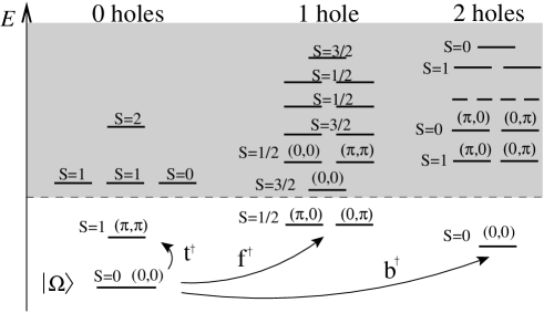
FIG. 2.: This figure is reproduced from Altman and Auerbach. The diagram displays the exact results from the exact diagonalization of a single plaquette. Aside from the undoped plaquette with singlet correlations (the vacuum $|\Omega\rangle$), the three lowest lying excited states (the triplet, the low energy fermion (the single hole), and the low lying boson (two holes)) are the the states of most relevance in the low energy sector of problem. In the low energy world, having a certain bar code pattern generally goes hand in hand with a high amplitude for the corresponding low energy eigenstates of the pattern associated with each of the individual plaquettes.

III A simple classification

Let us imagine that numerical results hint very strongly at a certain abbreviated ground state of the Hubbard or t-J model (e.g a bar code representation of the DMRG results of White and Scalapino along with a coarser covering toward the edges to better remove the effect of boundary conditions toward the edges). If a certain periodic abbreviated ground state appears with some period $L$ then the appearance of such a state and its cousins generated by translations (relying on the observed periodicity) on a finite $L\times L$ (or larger) slab $\lambda$ will be termed “good”. All other states not related by symmetry and not appearing in the numerical ground state will be defined as “bad”.

If the numerical results indeed reflect the true state of affairs and are not an artifact of spurious boundary conditions or other finite size effects, then in tiling the real physical infinite lattice $\Lambda$ with all maximally overlapping windows $\{\lambda\}$, we should observe many more “good” states than “bad”.

IV What are we after?

In a nutshell, we wish to show how we can bound the number of “bad” bar coded states in all maximally overlapping clusters $\{\lambda\}$ vis a vis the number of the “good” candidate states.

The bound that we will momentarily arrive at trivially reads

$$N_{b}\leq(\frac{\delta}{\Delta})N_{g}.$$ (5)

The quantities $\delta$ and $\Delta$ are gaps that we will detail below.

V The Means

Although not the most efficient, we will examine the energy of the system. The two gaps (or gap and anti-gap) $\Delta$ and $\delta$ are tied to the energy of the cluster $\lambda$ when subjected to open and periodic boundary conditions respectively. $\Delta$ denotes by (at least) how much the energy of any bar code configuration apart from the bar code sector of the true numerical ground state on the finite size cluster is elevated relative to the absolute energy minimum on the finite size cluster $\lambda$.

As will be shown below, a trivial lower bound on the energy of the system may be obtained by covering the entire lattice $\Lambda$ with all maximally overlapping finite blocks $\{\lambda\}$, consequently registering the bar code representation within each block $\lambda$, and finally summing the lower bounds on the energies of each of the bar code patterns that appear while tiling the system with all these maximally overlapping windows $\{\lambda\}$. The gap $\Delta$ computed by examining constrained open boundary condition minima is the lower bound on the energy increase each time a “bad” bar coded pattern is encountered.

A trivial upper bound on the true ground state energy of the infinite system may be obtained by merely minimizing the energy on a $\lambda$ subject to periodic boundary conditions. Obviously, the open boundary condition minimum will be lower (or the same) when compared to its periodic boundary condition counterpart. The difference between the two is denoted by $\delta$. As the size of the cluster $\lambda$ becomes larger and larger, the periodic boundary condition and open boundary condition must veer toward each other. Small delta ($\delta$) is indeed small for large enough $L$.

There is one detail which we have so far tucked away under the rug- in evaluating the energies on finite size cluster $\lambda$ we must renormalize the parameters $t,U,...$ such that the sum of the Hamiltonians on each individual cluster

$$H=\sum_{\{\lambda\}}h_{\lambda}$$ (6)

is the global Hamiltonian on the entire system $\Lambda$. The number of nearest neighbor pairs differs from the number of the number of sites and consequently the parameters associated with these (t and U respectively) must be readjusted. A similar occurrence happens if longer range (yet obviously finite) interactions are introduced.

VI Translational Symmetry

Translational symmetry is not broken in the scheme presented here. The reader will note that we examine all maximally overlapping blocks $\{\lambda\}$ in concert. We are not looking at a specific subset of clusters- that would indeed break translational symmetry.

This maximally overlapping covering is a bit non-traditional. Virtual hole evaporation and other processes that one might worry will not taken into account when examining small fragments of the cluster are very transparently accounted for by this and many other coverings. The maximal overlapping covering is more important for easily incorporating correctly longer range interactions (next nearest neighbor and beyond) The reader can invent a multitude of other variants.

VII Chemical Potential and Doping

Throughout the minimization procedures, the number of holes is not held fixed over each of the small clusters $\lambda$. A chemical potential term is inserted instead to provide the correct density of holes over the entire lattice $\Lambda$. The renormalization of the chemical potential term with the size of the block $L$ is identical to the scaling of the on-site Hubbard repulsion term $U$.

VIII Lower Bounds (via Constrained Open Boundary Condition Minima)

Here we give the reader a flavor of how constrained lower bounds may be easily generated and employed. In order to set the stage for things to come and to distill the essentials, we will start by examining the situation when the cluster $\lambda$ is the minimal single plaquette. Later on we will show how all of this may be trivially extended for larger covering clusters.

The state of the system is a linear combination of the states in the basis vectors in the Hilbert space spanned by

$$|e_{\alpha}^{\prime}\rangle=|1^{\prime}\rangle\otimes|2^{\prime}\rangle...\otimes|N^{\prime}\rangle,$$ (7)

where $|i^{\prime}\rangle$ specifies the state of the electron (including. its absence- i.e. a hole) at site $i$.

Now, let us imagine duplicating the basis vectors at every site. At each site $i$ we assign two basis vectors $|i^{A}\rangle$ and $|i^{B}\rangle$.

Let us furthermore define the even sublattice basis state by

$$|e_{A}\rangle=|Plaquette_{0}\rangle\otimes|Plaquette_{2}\rangle\otimes...$$ (8)

where each of the plaquettes $\{|Plaquette_{2n}\rangle\}$ lies in the even (A) sublattice.

Each plaquette basis state vector in the even sublattice is given by a direct product of the electronic basis state vectors at each one of its four sites

$$|Plaquette_{2k}\rangle=\prod_{i^{A}\in Plaquette_{2k}}|i^{A}\rangle$$ (9)

where, as before, $|i^{A}\rangle$ denotes the individual electronic state at site $i$.

Similar definitions and expressions may be written for the odd (B) sublattice.

As we must constrain

$$|i^{A}\rangle=|i^{B}\rangle$$ (10)

for each lattice site $i$, the Hilbert space spanned by

$$|e_{\beta}\rangle=|e_{A}\rangle\otimes|e_{B}\rangle$$ (11)

contains the physical Hilbert space of Eqn.(7) as a special subspace.

Now, let us write the full (range one Hubbard or t-J) Hamiltonian as

$$H=\frac{1}{2}(H_{A}+H_{B})$$ (12)

with $H_{A}$ having non-vanishing matrix elements only within the $\{|e_{A}\rangle\}$ (which is the same as the $\{|i_{A}\rangle\}$) subspace. Similarly, $H_{B}$ has matrix elements only within the $B$ subspace. The factor of one half in Eqn.(12) was inserted due to the doubling of degrees of freedom. Each electronic state makes an appearance twice- once in the $\{|i_{A}\rangle\}$ basis and once in the $\{|i_{B}\rangle\}$ basis. Now, note that the decomposition of Eqn.(12) is such that each Hamiltonian on the right hand side does not connect sites on different plaquettes- there are no inter-plaquette interactions in either $H_{A}$ or $H_{B}$. We may write

$$H_{A}=\sum_{k}h_{2k}$$ (13)

$$H_{B}=\sum_{k}h_{2k+1}$$ (14)

where $\{h_{n}\}$ are Hamiltonians that reside only in the local basis of the $n-$th plaquette.

As we increased the size of the Hilbert space, the minimum over the real physical Hilbert space is bounded from below by the minimum attained by its extended replicated counterpart:

$$\min_{|e_{\alpha}^{\prime}\rangle}\{H\}\geq\frac{1}{2}\Big{[}\min_{|e_{A}\rangle}\{H_{A}\}+\min_{|e_{A}\rangle}\{H_{B}\}\Big{]}$$ (15)

$$=\frac{N}{4}[\min\{h_{2k}\}+\min\{h_{2k+1}\}].$$ (16)

This is a trivial bound on the ground state energy of the system.

Suppose now that we were not interested in the global ground state but rather a restricted minimum. We can minimize the energy of the system subject to the constraint that within each odd plaquette we have one boson (hole pair) and within each even plaquette we have one hole. As the replicated Hilbert space is larger than the physical one (it includes the latter as a special subset) we will still trivially have

$\min_{|e_{\alpha}^{\prime}\rangle}\{H\}$ such that within each odd plaquette we have a hole pair and within each even plaquette we have a single hole $\geq\frac{N}{4}[\min\{h_{2k}\}$ such that we have one hole in the $2k$-th plaquette + $\min\{h_{2k+1}\}$ such that we have a hole pair in the $(2k+1)$-th plaquette $].$

All that we are doing above is tiling the lattice with dominos and for each of the two sides of the domino ($A$ and $B$) we find the minimum.

If we want to prove lower bounds on a more complicated commensurate structure (not a checkerboard one as we just considered now e.g. one with hole pairs on the red squares and single holes on the black squares) then we can consider clusters instead of single plaquettes and dominos.

Suppose that we want to prove that the ground state for a certain filling generates a certain commensurate pattern which occupies finite $(L\times L)$ blocks (clusters). To do that, we might naively consider all possible bar code sectors. However, that is not necessary. As we will detail in section(XI), it is sufficient to find the periodic boundary condition minimum (whatever it may be) and to combine it with the unrestrained open boundary condition minimum in order to obtain powerful bounds on a properly defined “good” sector that includes both minima.

The number of naive bar code sectors is exponential in the area of the cluster. This number is lowered by symmetry. The bulk of these bar code configurations are likely of high energy and the number of contenders for the low lying configurations might not be as forbidding. If we are examining natural potential candidates for the states appearing at 1/8 doping, the commensurability is very low and the number of various sectors is very small. Instead, for merely establishing a minimal gap $\Delta$, we can simply compute the global minima anywhere outside the “good” bar code sectors and compare to the unconstrained global minima (occurring, by definition in the “good” bar code states.

To proceed with the analysis of the $(L\times L)$ case, we generate $L^{2}$ replicas of the electronic state $|i^{\prime}\rangle$ at each site. We envision covering the lattice with all maximally overlapping $(L\times L)$ blocks $\lambda$. We may next define Hamiltonians $\{h_{\lambda}\}$ residing in the local subspace of the $L\times L$ block. For a fragment (cluster) of size $L\times L$ plaquettes, there is a multiplicative factor of $1/(L(L+1))$ that comes in the definition of $h_{\lambda}$ for a pure nearest neighbor (e.g. t-J) model when evaluating the energy of the entire system by summing over the energies in all maximally overlapping $L\times L$ blocks $\lambda$.

Similarly, for the Hubbard model, in tiling the entire plane by maximally overlapping small $L\times L$ fragments $\lambda$ each site (U) is over-counted $(L+1)^{2}$ times while each kinetic term (t) is over-counted $L(L+1)$ times. Consequently, for the Hubbard model, one will need to examine the readjusted values of $t,U$ on the single $L\times L$ fragment of plaquettes so as to produce the correct energies on the entire lattice.

By covering the lattice with all $L\times L$ fragments $\{\lambda\}$ and computing the energy within each fragment, and summing all of the lower bounds on the energies together, we may derive very generous lower bounds on the energies of the global system when the latter is subject to the demand that an $L\times L$ cluster if it belongs to a certain bar code sector.

It is important to emphasize that the bar code notation does not provide quantum numbers. The bar code values simply code in for rounded off values of the various expectation values. Each bar code configuration corresponds to many possible quantum states. Each individual state in the real physical Hilbert space also makes an appearance in the extended replicated Hilbert space (but not the converse). As a consequence, in performing a constrained minimum over a certain bar code sector or its complement, any state in the real physical Hilbert space that satisfies the correct expectation values bounds on the number occupancies etc. also makes an appearance in the replicated Hilbert space and therefore the minimum in the replicated space is lower (or the same) as that of the real unreplicated Hilbert space.

FIG. 3.: A covering of a fragment of the lattice with all maximally overlapping clusters $\{\lambda\}$. Here the various clusters are labeled by varying thickness. Each plaquette makes an appearance in $L^{2}$ different clusters $\lambda$. In the figure above $L=2$.

IX Upper bounds - via The Periodic Boundary Condition Problem

It is very easy to find an upper bound on the energy of a minimizing $L\times L$ configuration when the latter is embedded in the infinite lattice. We simply note that by the variational principle,

$$\langle\psi_{var}|H|\psi_{var}\rangle\geq\min_{|e_{\alpha}^{\prime}\rangle}\{H\}.$$ (17)

Now let us choose the variational wave-function $|\psi_{var}\rangle$ to be the one that minimizes the Hamiltonian on an $L\times L$ system when subjected to periodic boundary conditions. Non-uniform states can easily (and do in many problems) appear as periodic boundary condition minima; periodic boundary conditions merely constrain the components of the allowed wave-numbers to be integer multiples of $(2\pi/L)$. As $|\psi_{var}\rangle$ satisfies periodic boundary conditions, the $L\times L$ wave-function may trivially cover the entire macroscopic lattice. This state will belong to some sector. If it does not belong to the true macroscopic ground state pattern, we might need to increase $L$ until the periodic boundary condition minimum will lie in the “good” ground state sector of the system.

Just as in the discussion in the previous section, we will need to renormalize the interaction parameters in an open finite block $h_{\lambda}$ so that the sum of all these,

$$\sum_{\lambda}h_{\lambda}=H.$$ (18)

The normalization will be the same as in the previous case of the derivation of lower bounds. After all, when tiling the plane with all possible $(L\times L)$ blocks $\{\lambda\}$, the number of single points (U) and “bonds” (t or J) that are being counted is unique. The ground state of the entire system is trivially bounded from above by

$$N\epsilon_{good},$$ (19)

with

$$\langle\psi_{var}|h_{\lambda}|\psi_{var}\rangle=\epsilon_{good},$$ (20)

where the expectation value is now evaluated for $|\psi_{var}\rangle$ on the open $L\times L$ cluster.

(Notwithstanding, when periodic boundary conditions are employed, and the final periodic $L\times L$ system is unraveled to cover the entire lattice each site (with its associated interaction energy $U$ in the Hubbard model), and each link (with its associated kinetic energy (t) and (for the t-J model) its associated exchange energy J) appear in exactly $L^{2}$ different blocks $\{\lambda\}$.)

Explicitly, $\delta=L/(L+1)\times$ (the minimum on $\lambda$ with periodic boundary conditions when also including bonds connecting opposite boundaries) - (open boundary condition minimum on $\lambda$ when constrained to lie outside the “good” bar-code sector).

The factor of L/(L+1) originates from the fact that when tiling the plane with clusters $\lambda$ there are no interactions amongst opposite sides of $\lambda$ that can be accounted for. The computation for the open and closed boundary condition blocks are done on equal footing.

If $\epsilon_{good}$ is of lower value than the lower bounds (see the previous section) which we will obtain for all other “bad” sectors then we immediately prove that the ground state of the entire lattice is favorably ($N_{b}\leq N_{g}$) in the same sector as the periodic boundary condition minimum. That is, in each $L\times L$ window we will likely see the same pattern modulu trivial translations. If $\epsilon_{good}$ is not lower than the lower bounds on the other sectors, we might need to increase the size of our $L\times L$ blocks and re-compute upper and lower bounds.

That the two bounds should cross is to be expected for coarse covering as, in the large $L$ limit, the periodic boundary condition state becomes the true ground state of the system, and changing it to a different sector (altering any given plaquette(s) to a different bar code state) will entail a finite energy penalty.

X Putting all of the pieces together- Gaps and Antigaps

If the energy gap separating the open boundary condition minimum on all “bad” sectors from the periodic boundary condition minimum within the “good” sector is $\Delta$ and if the open boundary condition minimum (within the “good” sector) is lower by $\delta$ compared to the periodic boundary condition minimum, then if within the maximal tiling of the plane with all maximally overlapping clusters, the number of clusters lying within the “good” sector is $N_{g}$ and the number of clusters lying within the “bad” sector is $N_{b}$ then the energy difference between that configuration is elevated by at least

$$\overline{\Delta}\equiv[N_{b}\Delta-N_{g}\delta]$$ (21)

relative to the periodic boundary condition minimum.

In the limit of large cluster size, both the periodic boundary condition minimum and the open boundary condition minimum must match with that of the global ground state energy state: $\delta\to 0$.

For large enough clusters, the lower bound, $\overline{\Delta}$, on the energy penalty as compared to the true global ground state becomes meaningful. Only bad clusters of number

$$N_{b}\leq(\frac{\delta}{\Delta})N_{g}$$ (22)

will not elevate the ground state according to our bound (i.e. will not lead to $\overline{\Delta}>0$). By their very definition, the gaps must satisfy $\delta<\Delta$ if both the open and periodic boundary condition minima give rise to the same bar coded state(s), and $N_{b}$ is always smaller than $N_{g}$. The bounds become increasingly serious as the ration $(\delta/\Delta)$ diminishes.

Note that as the open boundary condition problem is not translationally invariant, we will in general find patterns that are related to each other by translations on the global lattice yet have different minimal energies on the open boundary condition problem on the fragment (cluster). In such a case, the bounds will even improve. If several good patterns have relative “anti-gaps” $\delta_{i}$ then for those we will replace $N_{g}\delta$ in the bound by the appropriate sum of $\{\delta_{i}\}$. In the most stringent bound, we may set, of course, $\delta\equiv\max_{i}\delta_{i}$.

Even if we have a finite size block $\lambda$ for which the periodic boundary condition and the open boundary condition minima lie in different abbreviated bar code sectors, the more “detailed balance” equation,

$$\sum_{\{\lambda_{i}\}}(\Delta_{i}-\delta_{i})\leq 0,$$ (23)

will lead to a strong constraint.

XI A Possible Via For Proving Stripes On the Infinite Lattice

If results similar to the end product of the DMRG calculations of White and Scalapino [1] are found for a system with both open and closed boundary conditions (similar to the pattern depicted in Fig.(4)) then the existence of stripes on the infinite lattice will effectively be proven for that Hamiltonian. All states with densities in between (and including) the two extremes (the periodic and open boundary condition minima) will occur (up to trivial translations) at least 50% of the time. The proof is trivial: both the open and closed boundary condition minima lie in the same sector (this is how we readjusted the definition of the “good” sector) and consequently $\delta<\Delta$. Inserted in Eqn.(22), this demonstrates that $N_{b}\leq N_{g}$- i.e. “good” charge order will be observed in more than a half of the blocks $\{\lambda\}$. In general, Eqn.(23) will impose restrictions on the form of the ground state.

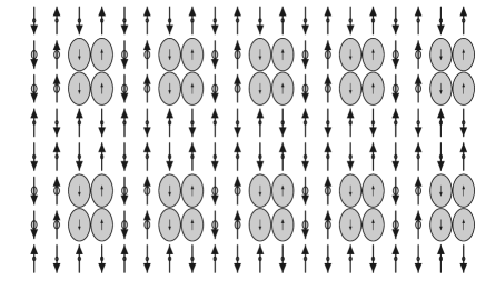
FIG. 4.: A bond centered stripe as attained in mean field theory. From M. Bosch et al. Earlier similar pictures were found by the detailed DMRG calculations of White and Scalapino.

If the stripes found by DMRG are a finite size artifact and indeed do result from the use of the open boundary conditions, then we can add additional short Coulomb repulsions (always present in the real system) to enhance non uniform charge order in both the open boundary condition problem (which already displays non-uniform order without this enhancement) and within the periodic boundary condition problem and to establish rigorous bounds on non-uniform charge and spin densities.

The real question is, of course, what system sizes are required before nonuniform charge order might be observed within the ground state of a system subjected to periodic boundary conditions. Periodic boundary conditions merely favor certain commensurate Fourier modes: non-uniform configurations do, of course, arise. Nevertheless, generically, charge density like oscillations within the ground state are far easier to observe in systems subject to open boundary conditions. If the commensurability is low, e.g. natural candidate ground states for 1/8 doping, then one might naively expect the periodic ground state not to deviate by much relative to that on an open fragment.

Acknowledgments

It is a pleasure to thank Assa Auerbach for numerous conversations and correspondence.

REFERENCES

- [1] S. R. White and D. J. Scalapino, Phys. Rev. Lett. 80, 1272 (1998), cond-mat/9907375
- [2] J. Zaanen and O. Gunnarsson, Phys. Rev. B 40, 7391 (1989); K. Machida, Physica C 158, 192 (1989); D. Poilblanc and T. M. Rice, Phys. Rev. B 39, 9749 (1989); H. J. Schulz, J. Physique, 50, 2833 (1989); M. Kato, K. Machida, H. Nakanishi, and M. Fujita, J. Phys. Soc. Jpn., 59, 1047 (1990); J. A. Verges et al., Phys. Rev. B 43, 6099 (1991); M. Inui and P. B. Littlewood, Phys. Rev. B 44, 4415 (1991)
- [3] V. J. Emery and S. A. Kivelson, Physica C 209, 597 (1993)
- [4] Ehud Altman and Assa Auerbach, Phys. Rev. B 65, 104508 (2002), cond-mat/0108087
- [5] M. Bosch, W. van Saarloos, and J. Zaanen, Phys. Rev. B 63,92501 (2001), cond-mat/0003236