THE PHYSICAL BASIS FOR PARRONDO’S GAMES

Abstract

Several authors [1, 2, 3, 4] have implied that the original inspiration for Parrondo’s games was a physical system called a “flashing Brownian ratchet [5, 6]” The relationship seems to be intuitively clear but, surprisingly, has not yet been established with rigor.

The dynamics of a flashing Brownian ratchet can be described using a partial differential equation called the Fokker-Planck equation [7], that describes the probability density, of finding a particle at a certain place and time, under the influence of diffusion and externally applied fields. In this paper, we apply standard finite-difference methods of numerical analysis [8, 9, 10] to the Fokker-Planck equation. We derive a set of finite difference equations and show that they have the same form as Parrondo’s games. This justifies the claim that Parrondo’s games are a discrete-time, discrete-space version of a flashing Brownian ratchet. Parrondo’s games, are in effect, a particular way of sampling a Fokker-Planck equation. Our difference equations are a natural and physically motivated generalisation of Parrondo’s games. We refer to some well established theorems of numerical analysis to suggest conditions under which the solutions to the difference equations and partial differential equations would converge.

The diffusion operator, implicitly assumed in Parrondo’s original games, reduces to the Schmidt formula for the integration of the diffusion equation. There is actually an infinite continuum of possible diffusion operators. The Schmidt formula is at one extreme of the feasible range. We suggest that an operator in the middle of the feasible range, with half-period binomial weightings, would be a better representation of the underlying physics.

Physical Brownian ratchets have been constructed and have worked [11, 12, 13, 14, 15]. It is hoped that the finite element method presented here will be useful in the simulation and design of flashing Brownian ratchets.

1 The Fokker-Planck equation

One of the classical problems of statistical physics, and physical chemistry, is to find a macroscopic statistical description for the diffusion of a dissolved molecule or ion in a uniform fluid solvent. The microscopic state of such a system has very many degrees of freedom, possibly even more than an Avogadro number of degrees of freedom. This gives rise to an equally large number of coupled equations of motion. It is completely impractical to solve such a large system with rigor. We must abandon the idea of an exact solution. We are forced to use a statistical description, where we can only describe the probability of certain events.

We denote the probability of finding a Brownian particle at a certain point on space, $z$, and time, $t$, by $p=p\left(z,t\right)$. The time-evolution of $p\left(z,t\right)$ is governed by a partial differential equation called the Fokker-Planck equation:

$$\frac{\partial^{2}}{\partial z^{2}}\left(D\left(z,t\right)p\left(z,t\right)\right)-\frac{\partial}{\partial z}\left(\alpha\left(z,t\right)p\left(z,t\right)\right)-\frac{\partial}{\partial t}p\left(z,t\right)=0~{}.$$ (1)

The functions $\alpha\left(z,t\right)$ and $D\left(z,t\right)$ are referred to as the infinitesimal first and second moments of diffusion. In practice, the infinitesimal second moment does sometimes depend on concentration of the solute, $p\left(z,t\right)$, but is usually regarded as constant and is called the “Fick’s law constant.” A typical value (for a hydrated sodium ion in water) would be of the order $D\approx 1.3\times 10^{-9}~{}\mbox{m}^{2}\mbox{s}^{-1}$. The infinitesimal first moment depends on the magnitude of externally imposed forces and on the mobility of the Brownian particle which is given by

$$u=\frac{Z_{e}}{6\pi\eta a}$$ (2)

where $Z_{e}$ is the electrical charge on the particle, $\eta$ is the kinematic viscosity of the solvent and $a$ is the effective radius of the particle. A typical value for the mobility (of a hydrated sodium ion in water) would be $u\approx 51.9\times 10^{-9}~{}\mbox{m}^{2}\mbox{s}^{-1}\mbox{volt}^{-1}$. Further descriptions and numerical data may be found in books on physical chemistry and statistical physics [16, 17, 18, 19]. If we apply an electrical potential, or voltage, of $V\left(z,t\right)$ then the infinitesimal first moment is given by

$$\alpha\left(z,t\right)=-u\frac{\partial}{\partial z}V\left(z,t\right)~{}.$$ (3)

The theory behind Equations 2 and 3 is due to Stokes and Einstein [20]. More information about the methods of solution and the applications of the Fokker-Planck equation can be found in Risken [7].

When we take into account the functional forms of $D$ and $\alpha$ then we can rewrite the Fokker-Planck equation as:

$$D\frac{\partial^{2}p}{\partial z^{2}}-\frac{\partial\alpha}{\partial z}p-\alpha\frac{\partial p}{\partial z}-\frac{\partial p}{\partial t}=0~{}.$$ (4)

This is the form of the Fokker-Plank equation which we will sample at regular intervals in time and space, to yield finite difference equations.

2 Finite difference approximation

Many Partial Differential Equations, or PDEs, including Equation 4, can be very difficult to solve analytically. One well established approach to this problem is to sample possible solutions to a PDE at regular intervals, called mesh points [8]. The true solution is approximated locally by a collocating polynomial. The values of the derivatives of the true solution are approximated by the corresponding derivatives of the collocating polynomial.

We can define local coordinates, expanded locally about a point $\left(z_{0},t_{0}\right)$ we can map points between a real space $\left(z,t\right)$ and an integer or discrete space $\left(i,j\right)$. Time, $t$, and position, $z$, are modelled by real numbers, $t,z\in\mathcal{R}$ and the corresponding sampled position, $i$, and sampled time, $j$, are modelled by integers $i,j\in\mathcal{Z}$. We sample the space using a simple linear relationship

$$\left(z,t\right)=\left(z_{0}+i\lambda,t_{0}+j\tau\right)$$ (5)

where $\lambda$ is the sampling length and $\tau$ is the sampling time.

In order to map Equation 4 into discrete space, we need to make suitable finite difference approximations to the partial derivatives. The notation is greatly simplified if we define a family of difference operators:

$$\Delta_{i,j}=p\left(z_{0}+i\lambda,t_{0}+j\tau\right)-p\left(z_{0},t_{0}\right).$$ (6)

In principle, this is a doubly infinite family of operators but in practice we only use a small finite subset of these operators. This is determined by our choice of sampling points. This choice is not unique and is not trivial. The set of sampling points is called a “computational molecule [8].” Some choices lead to over-determined sets of equation with no solution. Some other choices lead to under-determined sets of equations with infinitely many solutions. We chose a computational molecule called “Explicit” computation with the following sample points: $\left(i,j\right)\in\left\{(0,0),(-1,-1),(0,-1),(+1,-1)\right\}$.

We also need to make a choice regarding the form of the local collocating polynomial. This is not unique and inappropriate choices do not lead to unique solutions. A polynomial which is quadratic in $z$ and linear in $t$ is the simplest feasible choice:

$$p\left(z,t\right)=p\left(z_{0},t_{0}\right)+A_{1}\cdot\left(z-z_{0}\right)+A_{2}\cdot\left(z-z_{0}\right)^{2}+B_{1}\cdot\left(t-t_{0}\right)$$ (7)

where $A_{1}$, $A_{2}$ and $B_{1}$ are the real coefficients of the polynomial. Equations 5, 6 and 7 imply a simple system of linear equations that can be expressed in matrix form:

$$\left[\begin{array}[]{ccc}-\lambda&+\lambda^{2}&-\tau\\ 0&0&-\tau\\ +\lambda&+\lambda^{2}&-\tau\end{array}\right]\left[\begin{array}[]{c}A_{1}\\ A_{2}\\ B_{1}\end{array}\right]=\left[\begin{array}[]{c}\Delta_{-1,-1}\\ \Delta_{0,-1}\\ \Delta_{+1,-1}\end{array}\right]~{}.$$ (8)

These can be solved algebraically, using Cramer’s method to obtain expressions for $A_{1}$, $A_{2}$ and $B_{1}$:

$$A_{1}=\frac{p\left(z_{0}+\lambda,t_{0}-\tau\right)-p\left(z_{0}-\lambda,t_{0}-\tau\right)}{2\lambda}$$ (9)

and

$$A_{2}=\frac{p\left(z_{0}-\lambda,t_{0}-\tau\right)-2p\left(z_{0},t_{0}-\tau\right)+p\left(z_{0}+\lambda,t_{0}-\tau\right)}{2\lambda^{2}}$$ (10)

and

$$B_{1}=\frac{p\left(z_{0},t_{0}\right)-p\left(z_{0},t_{0}-\tau\right)}{\tau}~{}.$$ (11)

These are all intuitively reasonable approximations but their choice is not arbitrary. Equations 9, 10, 11 form a complete and consistent set. We could not change one without adjusting the others. We can evaluate the derivatives of Equation 7 to obtain a complete and consistent set of finite difference approximations for the partial derivatives:

$$\frac{\partial p}{\partial z}=A_{1}=\frac{p\left(z_{0}+\lambda,t_{0}-\tau\right)-p\left(z_{0}-\lambda,t_{0}-\tau\right)}{2\lambda}$$ (12)

and

$$\frac{\partial^{2}p}{\partial z^{2}}=2A_{2}=\frac{p\left(z_{0}-\lambda,t_{0}-\tau\right)-2p\left(z_{0},t_{0}-\tau\right)+p\left(z_{0}+\lambda,t_{0}-\tau\right)}{\lambda^{2}}$$ (13)

and

$$\frac{\partial p}{\partial t}=B_{1}=\frac{p\left(z_{0},t_{0}\right)-p\left(z_{0},t_{0}-\tau\right)}{\tau}~{}.$$ (14)

We can apply the same procedure to $\alpha\left(z,t\right)$ to obtain

$$\frac{\partial\alpha}{\partial z}=A_{1}=\frac{\alpha\left(z_{0}+\lambda,t_{0}-\tau\right)-\alpha\left(z_{0}-\lambda,t_{0}-\tau\right)}{2\lambda}~{}.$$ (15)

Equations 12, 13, 14 and 15 can be substituted into Equation 4 to yield the required finite partial difference equation:

$$p\left(z_{0},t_{0}\right)=a_{-1}\cdot p\left(z_{0}-\lambda,t_{0}-\tau\right)+a_{0}\cdot p\left(z_{0},t_{0}-\tau\right)+a_{+1}\cdot p\left(z_{0}+\lambda,t_{0}-\tau\right)$$ (16)

where

$$a_{-1}=\frac{\frac{D\tau}{\lambda^{2}}+\frac{\alpha\left(z_{0},t_{0}\right)\tau}{2\lambda}}{\frac{\alpha\left(z_{0}+\lambda,t_{0}-\tau\right)-\alpha\left(z_{0}-\lambda,t_{0}-\tau\right)}{2\lambda}\tau+1}$$ (17)

and

$$a_{0}=\frac{-2\frac{D\tau}{\lambda^{2}}+1}{\frac{\alpha\left(z_{0}+\lambda,t_{0}-\tau\right)-\alpha\left(z_{0}-\lambda,t_{0}-\tau\right)}{2\lambda}\tau+1}$$ (18)

and

$$a_{+1}=\frac{\frac{D\tau}{\lambda^{2}}-\frac{\alpha\left(z_{0},t_{0}\right)\tau}{2\lambda}}{\frac{\alpha\left(z_{0}+\lambda,t_{0}-\tau\right)-\alpha\left(z_{0}-\lambda,t_{0}-\tau\right)}{2\lambda}\tau+1}~{}.$$ (19)

We can overload the arguments of $p$ and write them in terms of the discrete space $\left(i,j\right)$ using the mapping defined in Equation 5.

$$p_{i,j}=a_{-1}\cdot p_{i-1,j-1}+a_{0}\cdot p_{i,j-1}+a_{+1}\cdot p_{i+1,j-1}~{}.$$ (20)

The meaning of the arguments should be clear from the context and from the use of subscript notation, $p_{i,j}$, rather than function notation, $p(z,t)$. Equation 20 is precisely the form required for Parrondo’s games.

3 Parrondo’s games

In the original formulation, the conditional probabilities of winning or losing depend on the state, $i$, of capital but not on any other information about the past history of the games:

• Game A is a toss of a biased coin:

  $$p_{win}=\frac{1}{2}-\epsilon$$ (21)

  where $\epsilon$ is an adverse external bias that the game has to “overcome”. This bias, $\epsilon$, is typically a small number such as $\epsilon=1/200$, for example [1, 3].

• Game B depends on the capital, $i$:

  If $(i\bmod 3)=0$

  , then the odds are unfavorable.

  $$p_{win}=\frac{1}{10}-\epsilon$$ (22)

  If $(i\bmod 3)\neq 0$

  , then the odds are favorable.

  $$p_{win}=\frac{3}{4}-\epsilon~{}.$$ (23)

It is straightforward to simulate a randomized sequence of these games on a computer using a very simple algorithm [4].

3.1 Game A as a partial difference equation

We can write the requirements for game A in the form of Equation 20.

$$p_{i,j}=\left(\frac{1}{2}-\epsilon\right)\cdot p_{i-1,j-1}+0\cdot p_{i,j-1}+\left(\frac{1}{2}+\epsilon\right)\cdot p_{i+1,j-1}~{}.$$ (24)

This implies a constraint that $a_{0}=0$ which implies that ${D\tau}/{\lambda^{2}}=1/2$ which defines the relative scales of $\lambda$ and $\tau$ so we can give it a special name:

$$\beta=\frac{D\tau}{\lambda^{2}}~{}.$$ (25)

The constraints on $a_{-1}$ and $a_{+1}$ imply a value for Parrondo’s “$\epsilon$” parameter:

$$\epsilon=\left\{\frac{\lambda}{4D}\right\}\alpha\left(z_{0},t_{0}\right)$$ (26)

which can be related back to an externally imposed electric field, $E=-\partial V/\partial z$ using equations 2 and 3:

$$\epsilon=\left(\frac{\lambda}{4D}\right)\left(\frac{Z_{e}}{6\pi\eta a}\right)\left(-\frac{\partial V}{\partial z}\right)~{}.$$ (27)

The small bias, $\epsilon$, is proportional to the applied external field which justifies Parrondo’s original intuition.

3.2 Game B as a partial difference equation

There is still zero probability of remaining in the same state which implies a constraint that $a_{0}=0$ which implies that we still have the same scale, $\beta=\frac{1}{2}$. If we are in state $i$ then we can denote the probability of winning by
$q_{i}=P\left(\mbox{win}|\mbox{initial position is}~{}i\right)$. We can write the difference equations for game B in the form:

$$p_{i,j}=q_{i-1}\cdot p_{i-1,j-1}+0\cdot p_{i,j-1}+\left(1-q_{i+1}\right)\cdot p_{i+1,j-1}~{}.$$ (28)

which, together with Equations 17, 18 and 19, gives

$$\frac{q_{i-1}}{1-q_{i+1}}=\frac{a_{-1}}{a_{+1}}=\frac{1+\frac{\lambda}{2D\tau}\alpha_{i,j}}{1-\frac{\lambda}{2D\tau}\alpha_{i,j}}$$ (29)

which implies that

$$\alpha_{i,j}=2\lambda\beta\frac{q_{i-1}-\left(1-q_{i+1}\right)}{q_{i-1}+\left(1-q_{i+1}\right)}~{}.$$ (30)

This can be combined with Equation 3 and then directly integrated to calculate the required voltage profile. We can approximate the integral with a Riemann sum:

$$V_{i}=-\frac{2\beta}{u}\sum_{k=0}^{i}\frac{1-\left(\frac{1-q_{k+1}}{q_{k-1}}\right)}{1+\left(\frac{1-q_{k+1}}{q_{k-1}}\right)}$$ (31)

so we can construct the required voltage profile for the ratchet which means that, given the values of $q_{i}$, it is possible to construct a physical Brownian ratchet that has a finite difference approximation which is identical with Parrondo’s games. We can conclude that Parrondo’s games are literally a finite element model of a flashing Brownian ratchet.

We note that game B, as defined here, is quite general and actually includes game A as a special case.

3.3 Conditions for convergence of the solution

We would like to think that as long as $\beta=D\tau/\lambda^{2}$ is preserved then the solution to the finite partial difference equation 20 would converge to the true solution of the partial differential equation 4, as the mesh size, $\lambda$ goes to zero. Fortunately, there is a theorem due to O’Brien, Hyman and Kaplan [21] which establishes that the numerical integration of a parabolic PDE, in explicit form, will converge to the correct solution as $\lambda\rightarrow 0$ and $\tau\rightarrow 0$ provided $\beta\leq\frac{1}{2}$. Similar results may also be found in standard texts on numerical analysis [8, 9, 10].

We see that Parrondo’s choice of diffusion operator, with $\beta=\frac{1}{2}$ is at the very edge of the stable region.

3.4 An appropriate choice of scale

There is a possible range of values for $\beta$. As $\beta\rightarrow 0$ we require the time step $\tau\rightarrow 0$ which means that the number of time steps required to simulate a given time interval, $T$, increases without bound $N_{\mbox{steps}}=T/\tau\rightarrow\infty$. It is computationally infeasible to perform simulations with very small values of $\beta$. On the other hand, the value of $\beta=1/2$ implied in Parrondo’s games is at the very limit of stability. In fact, the presence of small roundoff errors in the arithmetic could cause the the discrete simulation to diverge significantly from the continuous solution.

We propose that choosing $\beta=1/4$, in the middle of the feasible range, is most appropriate. If we consider the case of pure diffusion, with $\alpha=0$, then Equation 20 reduces to

$$p_{i,j}=\beta\cdot p_{i-1,j-1}+\left(1-2\beta\right)\cdot p_{i,j-1}+\beta\cdot p_{i+1,j-1}$$ (32)

and if we choose $\beta=1/4$ then this reduces to

$$p_{i,j}=\frac{1\cdot p_{i-1,j-1}+2\cdot p_{i,j-1}+1\cdot p_{i+1,j-1}}{4}$$ (33)

which is the same as Pascal’s triangle with every second row removed. The solution to the case where the initial condition is a Kronecker delta function, $p_{i,0}=\delta_{i,0}$ is easy to calculate:

$$p_{i,j}=\frac{1}{2^{2j}}\cdot\left({}^{2j}_{j+i}\right)=\frac{1}{2^{2j}}\cdot\frac{\left(2j\right)!}{\left(j+i\right)!\left(j-i\right)!}$$ (34)

which is a half period, or double frequency, binomial. We can invoke the Laplace and De Moivre form of the Central Limit Theorem which establishes a correspondence between Binomial (or Bernoulli) distribution and the Gaussian distribution to obtain

$$p_{i,j}=\frac{1}{\sqrt{2\pi\left(\frac{j}{2}\right)}}\exp\left(\frac{-i^{2}}{j}\right)~{}.$$ (35)

This expression is only approximate but is true in the limiting case as $j\rightarrow\infty$.

In the case where $\alpha=0$; the Fokker Planck Equation 4 reduces to a diffusion equation:

$$D\frac{{\partial}^{2}p}{\partial{z}^{2}}-\frac{\partial p}{\partial t}=0$$ (36)

Einstein’s solution to the diffusion equation is a Gaussian probability density function:

$$p\left(z,t\right)=\frac{1}{\sigma\sqrt{2\pi}}\exp\left(\frac{-z^{2}}{2\sigma^{2}}\right)$$ (37)

where the variance, $\sigma^{2}$, is a linear function of time:

$$\sigma^{2}=2Dt~{}.$$ (38)

It is possible to verify that this is a solution by direct substitution:

$$D\frac{{\partial}^{2}p}{\partial{z}^{2}} = \frac{\partial p}{\partial t}$$ (39)

$$= \left(\frac{-1}{2t}\right)\cdot\left(1-\left(\frac{z}{\sigma}\right)^{2}\right)\cdot p\left(z,t\right)~{}.$$ (40)

If we sample this solution in Equation 37 using the mapping in Equation 5 then we obtain Equation 35 again. This is an exact result. We conclude that the choice of $\beta=1/2$ is very appropriate for the solution to the diffusion equation. We suggest that this would also be true for the Fokker-Planck equation, in the case where $\alpha$ is “small.” The appropriate choice of $\beta$, given arbitrarily large, or rapidly varying, $\alpha$ is still an unsolved problem. In general, we would expect that much smaller values, $\beta\rightarrow 0$, would be needed to accommodate more extreme choices of alpha.

3.5 An example of a simulation

We simulated a physically reasonable ratchet with a moderately large modulo value, $M=8$. (The value for the original Parrondo’s games was $M=3$.) We used the value of $\beta=1/4$. The simulation was based on a direct implementation of Equation 20 in Matlab. We chose a sampling time of $\tau=12~{}\mu\mbox{s}$ and a sampling distance of $\lambda\approx 0.25\mu\mbox{m}$. The result is shown in Figure 1, where we indicate how the expected position of a particle can move within a Brownian flashing ratchet during four cycles of the modulating field. We can see a steady drift of the mean position of the particle in response to the ratchet action.

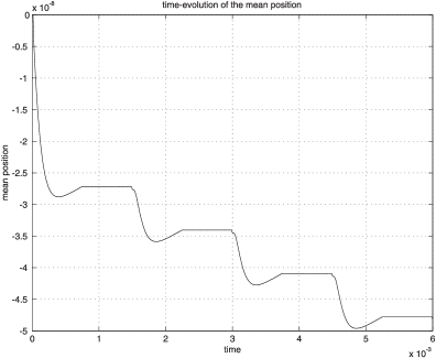
Figure 1: Time-evolution of the mean of the distribution $p(z,t)$. When the field is asserted, the mean position of the particles moves in a generally “downward” direction. There is some relaxation towards the end of that part of the cycle. When the field is turned off, the mean remains constant although diffusion causes the field to spread. The total shift in mean position of this ratchet is very modest, about $0.005~{}\mu$m, compared with the spacing between the teeth of the ratchet, of $2.0~{}\mu$m. Part of the motivation of this work is to optimise the transport effect of the Brownian ratchet, subject to constraints.

This simulation includes a total of 500 time samples. Note that the average rate of transport quickly settles down to a steady value, even after only four cycles of the ratchet.

4 Conclusions

We acknowledge the similar, but independent, work of Heath [22] et al. The focus of our paper is different. We seek to establish the physical, and mathematical, basis of Parrondo’s games and to derive a practical numerical technique for simulation.

We conclude that Parrondo’s games are a valid finite-element simulation of a flashing Brownian ratchet, which justifies Parrondo’s original intuition. We have established that Parrondo’s “$\epsilon$” parameter is a reasonable way to simulate a gradual externally imposed electric field, or voltage gradient. We have established that Parrondo’s implied choice of the $\beta$ parameter does lead to a stable simulation but we suggest that the choice of $\beta=1/4$ is more appropriate from a mathematical point of view.

Finally, we have generalised Parrondo’s games, in the form of a set of finite difference equations 20 and we have shown that these can be implemented on a computer.

References

- [1] G. P. Harmer and D. Abbott, Parrondo’s paradox, Statistical Science 14 { 2 } (1999) 206–213.
- [2] G. P. Harmer and D. Abbott, Parrondo’s paradox: Losing strategies cooperate to win, Nature 402 (1999) 864.
- [3] G. P. Harmer, D. Abbott and P. G. Taylor, The paradox of Parrondo’s games, Proc. Roy. Soc. Lond. A 456 { 1994 } (2000) 247–259.
- [4] G. P. Harmer, D. Abbott, P. G. Taylor and J. M. R. Parrondo, Brownian ratchets and Parrondo’s games, Chaos 11 { 3 } (2001) 705–714.
- [5] C. R. Doering, Randomly Rattled Ratchets, Il Nuovo Cimento 17D { 7 – 8 } (1995) 685–697.
- [6] C. R. Doering, L. A. Dontcheva and M. M. Klosek, Constructive role of noise: Fast fluctuation asymptotics of transport in stochastic ratchets, Chaos 8 { 3 } (1998) 643–649.
- [7] H. Risken, The Fokker-Planck Equation, Springer, Berlin (1985).
- [8] L. Lapidus, Digital Computation for Chemical Engineers, McGraw-Hill Book Co. Inc., New York (1962).
- [9] F. Scheid, Numerical Analysis, McGraw-Hill Book Co. Inc., New York (1968).
- [10] W. H. Press, S. A. Teukolsky. , W. T. Vetterling. and B. P. Flannery. Numerical recipes in C, Cambridge University Press, (1988).
- [11] L. P. Faucheux, L. S. Bourdieu, P. D. Kaplan and A. J. Libchaber, Optical thermal ratchet, Phys. Rev. Lett. 74 { 9 } (1995) 1504–1507.
- [12] G. W. Slater, H. L. Guo and G. I. Nixon, Bidirectional transport of polyelectrolytes using self-modulating entropic ratchets, Phys. Rev. Lett. 78 { 6 } (1997) 1170–1173.
- [13] D. Ertas, Lateral separation of macromolecules and polyelectrolytes in microlithographic arrays, Phys. Rev. Lett. 80 { 7 } (1998) 1548–1551.
- [14] T. A. Duke and R. H. Austin, Microfabricated sieve for the continuous sorting of macromolecules, Phys. Rev. Lett. 80 { 7 } (1998) 1552–1555.
- [15] J. S. Bader, R. W. Hammond, S. A. Henk, M. W. Deem, G. A. McDermott, J. M. Bustillo, J. W. Simpson, G. T. Mulhern and J. M. Rothberg, DNA transport by a micromachined Brownian ratchet device, PNAS 96 { 23 } (1999) 13165–13169.
- [16] R. B. Bird, W. E. Stewart, E. N. Lightfoot Transport Phenomena, John Wiley & Sons, New York (1960).
- [17] F. Reif, Statistical Thermal Physics , McGraw-hill Book Co.,Singapore (1965).
- [18] P. W. Atkins, Physical Chemistry, Oxford University Press, Oxford (1978).
- [19] E. L. Cussler, Diffusion; Mass transfer in fluid Systems, Cambridge University Press, Cambridge (1997).
- [20] A. Einstein, Investigations on the Theory of the Brownian Movement, Dover, New York (1956)
- [21] G. G. O’Brien, M. A. Hyman and S. Kaplan J. Math. Phys. 29 (1951) 223.
- [22] D. Heath, D. Kinderlehrer, Kowalczyk Discrete and continuous Ratchets: From Coin Toss to Molecular Motor, Website: http//math.smsu.edu/journal Discrete and Continuous Dynamical systems Series B 2 { 2 } (2002) 153–167.