“Vortex-melting front” in thin superconductors with pinning

Abstract

Magneto-optical observations of a second flux front, which occurs at the second peak in the magnetization of Bi₂Sr₂CaCu₂O_x single crystals related to the known first order “vortex-lattice melting”, are reconsidered. We show that, in thin samples, electrodynamics necessarily leads to an extended region in which the magnetic induction adopts a nearly constant value close to that at which the phase transition occurs at thermal equilibrium. In this region a dynamical phase mixture of vortex “solid” and “liquid” should exist. Interestingly, the observed second flux front does not mark the “melting” front, as it was naively interpreted earlier, but indicates the disappearance of the last “solid droplets”.

I Introduction

One of the most fascinating features of the vortex structure in layered superconductors is the so-called “melting” of the vortex ensemble. It is clearly established by now that this transition is a first-order phase transition above which the long-range correlation along the vortex lines is lost.[1] The most thoroughly investigated material, in which the “vortex melting” occurs well below the second critical field, is the high-$T_{c}$ superconductor Bi₂Sr₂CaCu₂O_x (BSCCO). There are attempts to add some other phase transition lines to the $B$-$T$ phase diagram of this material ($B$ is the local induction and $T$ the temperature). For example, the field of abrupt increase of the screening current with increasing $B$, the so-called second peak of the magnetization, was ascribed to a second order phase transition connected with the “melting” line at a tricritical point. However inspection of the available data suggests that the line of the second peak in the phase diagram is the continuation of the “melting” line into the low-temperature area where bulk currents do not completely relax during the experiment.[2]

It is natural to assume that, in spite of the macroscopic irreversibility, the vortex phases are in equilibrium locally. Then the unified “melting line” including the second peak-line, which shifts as one curve under the introduction of additional disorder and/or change of anisotropy by oxygen doping or electron irradiation, [2, 3] is the only first-order phase transition line. Recently the absence of the tricritical point at the border of observable pinning was elegantly demonstrated by unmasking the equilibrium magnetization step at the vortex melting point from the hysteretic magnetization using ac demagnetization. [4] This picture implies different pinning properties of these two vortex phases with correspondingly different current–voltage characteristics, which were extracted from local Hall probe measurements of the magnetic relaxation in the vicinity of the second magnetization peak at different temperatures and starting fields.[5] The resulting jump of the screening current at the first-order phase transition is then observed as a second front of the penetrating magnetic flux.

Magneto-optical observations of this second magnetization front initially did not bring much new information and did not attract enough attention. [6, 7] Such experiments were initially interpreted straightforwardly as the direct observation of the phase boundary which was already well established by local Hall probe measurements.[8, 5] However, after more careful consideration it became clear that the suggested “naive” interpretation is not compatible with the (macroscopic) electrodynamics of thin samples. Namely, in thin superconductors a sharp boundary between two different screening currents should produce the same logarithmic peak in the induction as at the sample edges. However, this moving peak is not observed in experiments. The correct theory indeed yields that a transition region with finite width and smooth current distribution should be expected, as it is known from the exact solutions for the penetration of perpendicular flux into thin samples, see e.g.  Ref. [9]. We propose here a model which predicts that this transition area in thin samples should inevitably contain a mixture of both phases.

A comprehensive description of the peculiarities of magnetic flux dynamics became particularly important when new observations of metastable vortex phases under fast remagnetization were reported. [10, 11] In order to separate new dynamic effects from the (already complicated) geometry-dependent “regular” flux dynamics occurring when the vortex phases are in local equilibrium, we make a step backward in our investigations and describe the equilibrium case more carefully. The nature of flux flow at the phase transition is simulated qualitatively using an algorithm developed for the flux dynamics in thin conductors with nonlinear current-voltage law. [12]

II Magneto-optical observations

The penetration of a magnetic field into BSCCO single crystals was visualized by means of the magneto-optical imaging technique using a ferrimagnetic garnet indicator film with in-plane anisotropy. [13, 14, 15] In general, higher light intensity in the image means higher local magnetic induction normal to the sample surface. The images were recorded by a CCD camera during the continuous ramp of the perpendicular magnetic field with $dB_{a}/dt=200$ G s^-1 and digitalized every 250 ms by a video-frame grabber card. The camera was working at the standard TV frame frequency of 25 Hz, so each image of the obtained movie is an average over about 40 ms. The increase of $B_{a}$ during the acquisition of a single image is comparable to the measurement noise. The relatively fast ramp of the field was used in order to observe the critical slope of the initial penetration, which otherwise relaxes. The intensity profiles measured across the digital images were calibrated in terms of field units using an additional recording under equivalent conditions but above $T_{c}$. A separate calibration curve was obtained from the additional “empty” images for each point on the flux profiles. In this way we reduce the effect of inhomogeneities in the illumination and in the sensitivity of the indicator across the image. For demonstration, an underdoped BSCCO crystal grown at the FOM-ALMOS center (the Netherlands) by the traveling-solvent floating zone technique under 130 mbar O₂ partial pressure[16] was specially selected for the uniformity of flux penetration and for the low field $B_{\rm sp}\approx 180$ G at which the second magnetization peak occurs. The crystal was cut into a rectangle with dimensions $1450\times 700\times 43\,\mu$m³.

The initial penetration into the zero-field-cooled sample resembles the numerous magneto-optical observations of the Bean-like critical states in type-II superconductors. The crystal edges are well observed as a sharp change from the very bright field outside the sample and the grey interior. The flux penetrating from the crystal edges is visible as a grey belt (higher brightness represents higher

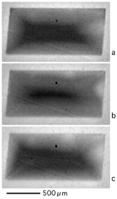
FIG. 1.: Magneto-optical imaging of the flux penetration into a zero-field-cooled BSCCO single crystal at $T=28.8$ K in continuously ramped $B_{a}$ with ramp-rate of 200 G s^-1. In every image, light areas correspond to high induction, while dark areas have low induction; however, the intensity-to-induction mapping (look-up table) in different images is selected separately in order to reveal specific details. Selected snapshots from the movie: (a) $B_{a}=200$ G, ordinary flux front below $B_{\rm sp}$. The dark area in the center is the Meissner area with $B=0$, the bright area around the crystal corresponds to the applied field $B_{a}$ and the grey belt at the edges represents the classical Bean-like penetration with a critical slope of $B$. (b) $B_{a}=300$ G: the second flux front appears as a new, sharp increase of the image brightness at the top and right sample edges, while the initial field profile persists in the sample center. (c) $B_{a}=450$ G: the second flux front above $B_{\rm sp}$. Note that the dark central part now corresponds to $B\sim B_{\rm sp}$, unlike the similar frame (a), where this value is represented by a light grey tone. The calibrated flux profiles for the entire image sequence, shown in Fig. 2, are taken along a vertical line crossing the sample at its center downwards.

local value of the perpendicular magnetic induction) which squeezes the central (dark grey) Meissner area in which $B$ is zero (Fig. 1 a). The gradual decrease of the brightness of the penetrated perimeter corresponds to the well-known Bean gradient of the penetrating flux. When the field at the edges reaches $B_{\rm sp}$, a second sharp flux front starts to penetrate from the crystal edges (Fig. 1 b). [6, 7, 11] When the second flux front has penetrated deep into the sample, the resulting image is becoming nearly identical to the initial penetration (compare Fig. 1 a and b). However, one should remember that the induction in the central dark area in Fig. 1 c approximately corresponds to that in the light grey field outside the sample in Fig. 1 a, where $B=0$ in the center.

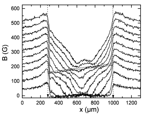
FIG. 2.: Magnetic flux profiles across the sample shown in Fig.1 at $T=28.8$ K. The field of the first order “vortex melting” is indicated by two dashed lines. The position of the sample edges is marked by vertical dotted lines with arrows at the abscissa. The profiles represent a sequence of images taken every 0.25 s, i.e., at intervals $\Delta B_{a}=50$ G. The images for the profiles number 4, 6 and 9 (counting from the bottom) are shown in Fig.1 a, b, and c, respectively.

The whole course of flux penetration during field ramping from zero to 500 G is visualized in Fig. 2 by $B(x)$ profiles measured across the sample width. After reaching a well-determined field level the increase of the induction $B$ pauses and $B$ is stabilized until a new flux front approaches which increases $B$ further. The plateau of constant induction is associated with the phase transition at $B_{\rm sp}$. The slight inclination of this plateau, which is marked by two dashed lines, is due to inhomogeneity of the crystal. To our knowledge, such inhomogeneity is found in all BSCCO crystals and is inevitable (see e.g. Refs. [17, 18]). During the subsequent decrease of the field a similar feature appears at the same line $B_{\rm sp}$ without notable hysteresis in the transition field. The second flux front looks very similar to what the ordinary Bean-like flux profile would have looked like if some flux relaxation had occurred during a temporal halt of the field ramp. Another close analogy exists with respect to flux penetration into a superconductor after field cooling. That analogy, in particular, shows that the initial interpretation of the second front as a phase boundary separating regions with very different critical currents, is not compatible with the perpendicular geometry of the experiment. Such a sharp border between two currents at a definite field is possible only in the longitudinal geometry, where it occurs at the junction of two different field gradients. In perpendicular geometry, however, any flux front penetrating into a thin superconductor is accompanied by strong sheet currents inside the screened area. [9, 19]

III Model calculations and discussion

In order to understand the experimental observations, let us first consider the simplest possible situation of a superconducting strip occupying $|x|<a$, $|z|<d/2$ ($d\ll a$) in which the vortex matter undergoes a first order transition at $B_{z}=B_{\rm sp}$. In the vortex solid below $B_{\rm sp}$, the critical current is zero, and in the vortex liquid above $B_{\rm sp}$, it has some non-zero value $J_{c}$. In other words, the critical current discontinuously jumps from zero to $J_{c}$ as the vortex matter melts. Furthermore, let us neglect surface and geometrical barriers. The flux penetration into this strip is illustrated in Fig. 3. As long as the applied field $B_{a}\parallel z$ does not exceed $B_{\rm sp}$, the strip is perfectly transparent to the field (flat profiles 1 and 2 in Fig. 3). Once the applied field exceeds $B_{\rm sp}$, the internal induction is stabilized at the value $B_{\rm sp}$, and further flux penetration is screened by a non-zero $J(x)$. The distribution of this $J(x)$ and of the internal induction are described by the well–known solution of Ref. [9]:

$\displaystyle\begin{array}[]{ccc}J(x)&=&\!\left\{\begin{array}[]{ll}\left(2J_{c}/\pi\right)\arctan\frac{cx}{\sqrt{b^{2}-x^{2}}},&~{}~{}~{}~{}|x|<b\\ J_{c}x/|x|,&~{}~{}~{}~{}b<|x|<a\end{array}\par\right.\\ &&\\ B(x)&=&\left\{\par\begin{array}[]{ll}B_{\rm sp},&~{}|x|<b\\ B_{\rm sp}+B_{c}{\rm arctanh}\frac{\sqrt{x^{2}-b^{2}}}{c|x|},&~{}b<|x|<a\\ B_{\rm sp}+B_{c}{\rm arctanh}\frac{c|x|}{\sqrt{x^{2}-b^{2}}},&~{}|x|>a\end{array}\par\right.\par\end{array}$

where $B_{c}=\pi\mu_{0}J_{c}/d$ is the characteristic field, $\pm b=a/\cosh[(B_{a}-B_{\rm sp})/B_{c}]$ is the position of the flux front, and $c=\sqrt{a^{2}-b^{2}}$. For Fig. 3, we chose $B_{c}=\frac{1}{2}B_{\rm sp}$. The situation is illustrated by the profiles 3 and 4. In the region in which $B>B_{\rm sp}$, the current $J=J_{c}$, while in the region with $B=B_{\rm sp}$, the strip geometry imposes the smooth decrease of $J$ to zero in the interval between the “second” flux front and the sample center. While it is evident that the former region is occupied by the high field vortex liquid, the latter region must also consist of vortex liquid, since the vortex solid (with zero critical current) cannot sustain the non-zero $J(x)$. Therefore, the observed flux front does not correspond to the front of phase transformation.

The above consideration, based on the simple Bean model, does not account for a non-zero current in the solid phase, nor for the possibility of flux creep. We include these effects using the algorithm previously developed for studying the flux penetration into thin superconductors with a nonlinear current–voltage law $E(J,J_{c})=\rho_{0}|J/J_{c}|^{\sigma}J$ where $J$ is the sheet current (the current density integrated over the strip thickness). [12] We model the sharp jump of the current-voltage law from $E^{-}(J)=E(J,J^{-}_{c})$ in the low-field low-pinning phase ($J_{c}=J^{-}_{c}$) to $E^{+}(J)=E(J,J^{+}_{c})$ in the high-field high-pinning phase ($J_{c}=J^{+}_{c}$) by introducing a step in $J_{c}(B)$ at the transition field $B_{\rm sp}$:

$$J_{c}(B)=J_{c0}+\frac{\Delta J_{c}}{2}\tanh\frac{B-B_{\rm sp}}{\Delta B}\,,$$ (1)

with jump width $\Delta B\ll B_{\rm sp}$ and jump height $\Delta J_{c}=J^{+}_{c}-J^{-}_{c}$. Other models of steps in the current–voltage characteristics, e.g. a jump in the creep exponent $\sigma(B)$, or different values of the parameters, give qualitatively similar results.

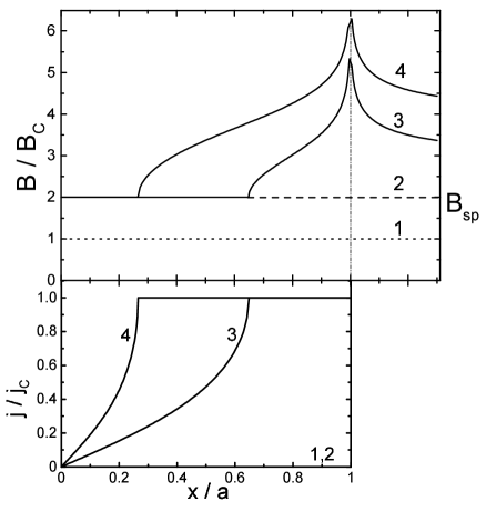
FIG. 3.: A simplified model for the flux penetration in the presence of a first order vortex matter phase transition. the critical current is zero for $B<B_{\rm sp}$ and equal to 1 for $B>B_{\rm sp}$. Profiles 1 to 4 correspond to $B_{a}=B_{c}$, $2B_{c}$, $3B_{c}$, and $4B_{c}$. The field $B_{\rm sp}$ is equal to $2B_{c}$.

The following graphs (Fig. 4 a–c) show profiles (across the strip) of the magnetic field $B(x)$, screening current $J(x)$, and the electric field $E(x)$ under a constant ramp rate of the external field $dB_{a}/dt=1$ for $\sigma=20$, $B_{\rm sp}=1$, $\Delta J_{c}=0.5$ and $\Delta B=0.04$, in dimensionless units where $J^{+}_{c}=1$ (critical sheet current), $a=1$ (half width of the strip), $B=H$, $dE/dx=dB/dt$ (left-hand coordinate system), and $\rho_{0}=1$. Our computed profiles of the induction $B(x)$ (Fig. 4a) well resemble the experimental profiles (Fig. 2). The initial penetration at $B<B_{\rm sp}$ is the same as was calculated analytically [9] and numerically [12]. As usual, the corresponding $J(x)$ in the flux penetrated area saturates at the “spatial projection” $J_{sat}^{-}$ of the low field current–voltage characteristic. The reason for this is very simple: after the complete penetration of the field, $B$ increases everywhere with the same constant rate. From the Maxwell law $dE(x)/dx=dB(x)/dt$ it follows that $E^{-}(J^{-}_{\rm sat}(x))=x\,dB_{a}/dt\propto x$ everywhere. Thus $J^{-}_{\rm sat}(x)=$ $J^{-}(x\,dB_{a}/dt)$, where $J^{-}(E)$ is the inverse function of

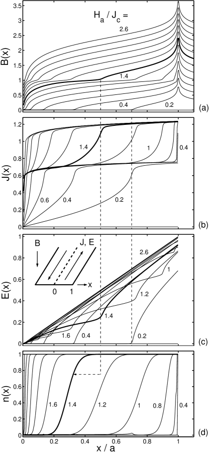
FIG. 4.: Computed flux penetration into a superconducting strip with a sharp jump of the critical current from $J^{-}_{c}=0.75$ to $J^{+}_{c}=1.25$ at the vortex-lattice phase-transition field $B_{\rm sp}=1$: (a) perpendicular induction $B(x)$, (b) screening sheet current $J(x)$, (c) electrical field $E(x)$, and (d) relative concentration of the two phases $n(x)$ for $B_{a}=0.2$, 0.4, $\dots$ 2.6. The right dashed vertical line indicates the well-known initial penetration front at $B_{a}=0.2$ with a sharp decrease of $J(x)$ from the critical value $J^{-}_{\rm sat}\approx 0.7$ and $E(x)$ dropping to zero. To illustrate the correlation between $B(x)$, $J(x)$, $E(x)$ and $n(x)$ during “vortex melting”, the profiles at $B_{a}=1.4$ are marked as bold lines. $B(x)$ clearly exhibits a second flux front on top of $B_{\rm sp}=1$, starting at the left vertical dashed line, where $J(x)$ sharply decreases from $J^{+}_{\rm sat}\approx 1.2$ towards $J^{-}_{\rm sat}\approx 0.7$ and $E(x)$ has a sharp kink. But the corresponding change of $n(x)$ extends much farther towards the center, as indicated by an arrow pointing from the second front to the left. The inset in (c) shows the geometry. All values $B$, $J$ and $E$ are given in the dimensionless units $J_{c}$ (see the text).

$E^{-}(J)$ defined below $B_{\rm sp}$. The constant critical current of the classical Bean model corresponds to the nearly constant flat part of $J^{-}_{\rm sat}(x)\approx J^{-}_{\rm sat}$. Unlike the Bean model, in our more realistic model the abrupt change of direction of the critical current at $x=0$, the so-called discontinuity line (d-line),[20] has a finite thickness. The transition from $+0.8J^{-}_{\rm sat}$ to $+0.8J^{-}_{\rm sat}$ extends over $\Delta x_{d}\approx 2\,E^{-}(0.8\,J^{-}_{c})/(dB_{a}/dt)$. For the particular $E(J)$ used in our simulations (Fig. 4) $\Delta x_{d}\approx 0.02a$.

When $B$ increases further and approaches the value $B_{\rm sp}$, the field gradient decreases, and further flux penetration occurs via the penetration of a new flux front moving on top of the line $B\approx B_{\rm sp}$. It is important to note that, as in the simplified case outlined above, the screening current $J(x)$ does not jump sharply at the flux front but changes smoothly from $J^{-}_{\rm sat}(x)$ to the new saturation $J^{+}_{\rm sat}(x)\approx J^{+}_{\rm sat}$ before the second front has arrived (Fig. 4b). Here again $E^{+}(J^{+}_{\rm sat}(x))=x\,dB/dt\propto x$ yields the “spatial projection” $J^{+}_{\rm sat}(x)$ of the high-field current-voltage law. This behavior is valid for any pair of functions $E^{-}(J)$ and $E^{+}(J)$, which play the role of saturation profiles of the sheet current $J(x)$ after the complete penetration of the field, below and above $B_{\rm sp}$, correspondingly. Preceding the second front there is a region where the flux density is nearly constant in space and time, $B(x,t)\approx B_{\rm sp}$ (Fig. 4 a); in this region the slope of the electric field is reduced since $dE/dx=dB/dt$ is small. In order to reach its final saturation shape $E(x)=x\,dB_{a}/dt$, $E(x)$ exhibits a sharp upward bend at the second flux front, which is clearly seen in Fig. 4c. We should mention that a non-zero $\Delta B$ is included here only for the stability of the numerical algorithm; its value only affects the rounding of sharp features in the flux profile for $B\approx B_{\rm sp}$, but not, as we checked, the wide smooth transition of the current. The simplified solution outlined above shows that the smooth transition in $J$ exists for $\Delta B=0$ as well.

Within the framework of our assumption that only two phases with fixed current–voltage laws $E^{-}(J)$ and $E^{+}(J)$ can exist in the superconductor, the above outlined smooth transition of the resulting $J(x)$ between the corresponding saturation profiles can be explained only by a phase mixture. One can imagine various configurations of the phase domains corresponding to different conditions, varying from the equality of $E$ in the two phases to the homogeneity of $J$. In general the dynamics of the corresponding phase mixture should be solved, but this complication is outside the scope of our paper. Here, we present the simplest and most natural model in which the intermediate region consists of narrow lamellar domains of alternating phases oriented parallel to the flux flow, i.e.perpendicular to the current, across the width of the strip. This model corresponds to homogeneous $J$ across the phase boundaries and a modulated $E$. In the mixed region, we then have $J_{\rm liquid}=$ $J_{\rm solid}=$ $J(x)$ and $E(x)=nE^{+}(J(x))+(1-n)E^{-}(J(x))$. Here, $n=n(x)$ is the relative concentration of one phase; $n=0$ corresponds to the “vortex solid” and $n=1$ to the “vortex liquid”. From the calculated $J(x)$ and $E(x)$ we obtain $n(x)$ in the form

$$n(x)=\frac{E(x)-E^{-}(J(x))}{E^{+}(J(x))-E^{-}(J(x))}$$ (2)

(see Fig. 4d). In case of the simplest domain structure of the phase mixture, equal parallel lamellae along the flux flow, the relative width of the “liquid” domains is equal to $n(x)$. An example of such domains at $B_{a}=1.4$ is shown in Fig. 5, which is obtained by flipping the corresponding profile $n(x)$ (outlined by the bold line in Fig. 4c) several times and cutting it at the right at the position of the second flux front, and at the left, e.g. at a value $n(x)=0.01$ ($0.01$ is an arbitrary choice, the final result depends on it logarithmically).

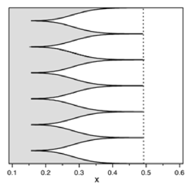
FIG. 5.: Scheme of the phase lamella preceding the second flux front marked here by a vertical dotted line that corresponds to the left dashed line in Fig. 3. The front moves from the right to the left. The “liquid phase” (right, white) interpenetrates the “vortex solid” (left, light grey). The vertical scale is not given by our theory.

Interestingly, “melting” (i.e. $n(x)>0$) starts well before the second flux front has arrived, and the second flux front corresponds not to the midpoint $n=\frac{1}{2}$, but to the point where $n(x)$ has already well saturated to $n=1$. At this point the “melting” transition is complete. The smooth transition of the current is characterized by the fast flux flow through the weaker “solid” lamella (light grey), the width of which plays the role of a “flux valve”, while the vortices in the “liquid” lamella (white) are nearly immobile until the second flux front arrives. At $x\lesssim x_{\rm sp}$, the average electric field equals

$$E(x)\approx E_{\rm sp}=\int_{0}^{x_{\rm sp}}{dB(x,t)\over dt}dx\approx{\rm const}$$

because $B(x,t)$ is fixed to a value $\sim B_{\rm sp}$. The vortex flow through the region of the phase mixture is concentrated in the “solid” phase. The local electric field (vortex velocity) in the solid is very high, $E_{\rm solid}=E^{-}(J(x))=E_{\rm sp}$, because the electric field in the “liquid” phase $E_{\rm liquid}=E^{+}(J(x))$ is nearly zero. Consequently, the width of the “solid” valve adapts itself so that the necessary average flux flow is conserved, i.e. $1-n_{\rm sp}\approx E_{\rm sp}/E_{\rm solid}$.

Particularly impressive is the moment when the second front approaches and the high second critical current $J^{+}_{\rm sat}$ passes through the “weak” “solid” phase. Here all necessary flux flow squeezes into the very narrow “solid neck” with a huge speed corresponding to $E^{-}(J^{+}_{\rm sat})$. The order of the introduced values $E_{\rm liquid}$ and $E_{\rm solid}$ can be read from the “spatial projections” of $E^{+}(J)$ and $E^{-}(J)$ in Fig. 4b (see the corresponding lower and upper asymptotics $J^{+}_{\rm sat}(x)$ and $J^{-}_{\rm sat}(x)$). For this one has to take a horizontal projection of, for example, the cross-point of the bold line $J(x)$ (at $B_{a}=1.4$) and the vertical dashed line, indicating the second flux front, onto $J^{+}_{\rm sat}(x)$ and $J^{-}_{\rm sat}(x)$. Then the first one will give $x^{+}=E_{\rm liquid}\sim 0.05$ and the second one will be well outside the graph at the right $x^{-}=E_{\rm solid}\sim 10^{3}$. The relative width of the “solid neck” is here $1-n_{\rm sp}\sim 2\times 10^{-4}$. In reality, even for such domains as thick as the sample the “neck” width given by our qualitative theory is well below the vortex spacing of 0.3 $\mu$m at $B_{\rm sp}$. This means that probably only a single line of “solid” vortices will move before the second front arrives.

The proposed dynamical intermediate structure of the coexisting phases should not be confused with the ordinary intermediate phase that exists at any first order magnetic phase transition in the narrow field range $\Delta B=B^{+}-B^{-}$ over which the jump occurs. The relative size of the equilibrium domains $n_{\rm eq}$ in that well known static case is fixed by the condition that the average local field equals the $B(x)$ which is determined by the entire current distribution, $n_{\rm eq}B^{+}+(1-n_{\rm eq})B^{-}=B(x)$.

As opposed to this, in our case the relative phase ratio $n(x)$ is determined by the different dynamics of the flux flow in the two different phases and by the global electrodynamics of the system, see the profiles in Fig. 4d and Eq. (2). In the ordinary static case, the region of the coexisting phases may be very narrow because $\Delta B$ is much smaller than the typical variation of $B(x)$ over the sample; its width equals $(dB/dx)^{-1}\Delta B$ at the phase transition. In our case the width of the transition region containing the phase mixture is a sizable fraction of the sample size, while our dynamic $B(x)$ varies even more due to the presence of high bulk currents.

The question arises whether the intermediate structure of dynamically coexisting solid and liquid vortex phases also occurs in thick samples (thicker than the penetration depth $\lambda$). In the case of the simplified model with zero current for $B<B_{\rm sp}$ and a critical current $J_{c}$ for $B>B_{\rm sp}$, we refer to Ref. [21], in which it is shown that the shape of the flux front in the interior of a thick superconductor is very well described by the shape of the current profile in an infinitely thin superconductor. Using Fig. 3, we can thus immediately draw the current front inside a thick sample. The region between this front and the sample surface carries a current $J_{c}$ and must therefore be in the liquid state. From the Bean model only, there is no objection to the inner core remaining in the solid state with $J_{c}=0$. In that case, one would also have a coexistence of solid and liquid phases, but now across the sample thickness. Such a scenario would depend on the stability of the curved phase boundary — any phase mixture in the inner core up to its complete transformation to the solid phase also does not contradict to electrodynamics.

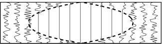
FIG. 6.: Hypothetical phase front between the vortex solid and the vortex liquid in a thick sample in the situation where the solid cannot sustain any current flow, and the liquid has a non-zero critical current. The shape of the front just corresponds to that of the current profile 3 in the lower panel of Fig. 3.

Recently, a real-time differential treatment of magneto-optical images allowed to visualize the propagating vortex “melting” front through a BSCCO crystal as a contour of the related equilibrium magnetization jump. [17, 18] The melting point appeared to be very sensitive to tiny inhomogeneities of the sample defect disorder and a very irregular “vortex melting” with no sign of equilibrium domains is observed even in the best crystals. Our lamella should be more robust because they are determined by the critical currents, which are much higher than the tiny equilibrium current drop at the “vortex melting” point. But unfortunately, the elaborate procedure of such observations cannot be applied to our case of irreversible magnetization. Very recently, after preparation of this paper, a mixture of phases with different $E(J)$ has been observed in the peak effect region in NbSe₂ using a scanning Hall probe magnetometer and local ac excitation. [22, 23] We have to mention that the phenomenon observed there, is static and the suggested model of the “vortex capacitor” differs from our dynamic model. Furthermore, we deal with an equilibrium transition, contrary to the metastable state considered in Refs. [22] and [23]. The new observation technique, nevertheless, may be applicable to our case; its magneto-optical imaging counterpart can be realized as well. Note however that in our case the picture is evolving rapidly (on the time scale of 10^-2 s) and the irreversible currents which would screen the small ac excitation are much higher.

IV Conclusions

We have obtained experimental and numerical flux profiles that render the major features of flux flow at “vortex-lattice melting” in the presence of pinning and magnetic hysteresis. The flux profiles show a second front corresponding to the well-known second peak in the magnetization curve. In thin superconducting plates, “melting” occurs well before the arrival of the second flux front. At that moment, the phase transition is complete and the low-field phase (“vortex solid”) with lower $J_{c}$ completely disappears there. The appearance of the high field phase (“vortex liquid”) does not produce any sharp feature on the observable field profiles. Rather, there is a large region preceding the second flux front in which domains of “solid” and “liquid” coexist dynamically: the relative width of these domains is controlled by the electrical field induced by the vortices moving under the force exerted by the current, which flows continuously across the domains; the current in its turn is controlled by the overall electrodynamics of the system. This intricate feature should be taken into account in a correct interpretation of experiments.

Evidently this effect occurs for any flux dynamics in the presence of a first order phase transition, irrespective of whether it is driven by ramping the applied field as in the presented experiment, or it happens during magnetic relaxation as in Ref. [10, 11]. Moreover, when the process is slow and the current in the “weak” “solid vortex-lattice” phase is allowed to relax to zero, the “melting” proceeds nearly immediately everywhere because the flux flow required for this is very low. In this case the remaining “solid” lamella should be very narrow and the second front moves on top of the nearly homogeneous “liquid” without any relation to the phase transition itself.

The authors are grateful to Ming Li and P.H. Kes of the FOM-ALMOS center (the Netherlands) for the samples. M.V.I. acknowledges financial support by the Max-Planck-Gesellschaft.

REFERENCES

- [1] E. Zeldov, D. Majer, M. Konczykowski, V.B. Geshkenbein, V.M. Vinokur, and H. Shtrikhman, Nature (London) 375, 373 (1995).
- [2] B. Khaykovich, E. Zeldov, D. Majer, T.W. Li, P.H. Kes, and M. Konczykowski, Phys. Rev. Lett. 76, 2555 (1996).
- [3] B. Khaykovich, M. Konczykowski, E. Zeldov, R.A. Doyle, D. Majer, P.H. Kes, and T.W. Li, Phys. Rev. B 56, 517 (1997).
- [4] N. Avraham, B. Khaykovich, Yu. Myasoedov, M. Rappaport, H. Shtrikhman, D.E. Feldman, T. Tamegai, P.H. Kes, M. Li, M. Konczykowski, K. van der Beek, and E. Zeldov, Nature (London) 411, 451 (2001).
- [5] M. Konczykowski, S. Colson, C.J. van der Beek, M.V. Indenbom, P.H. Kes, and E. Zeldov, Physica (Amsterdam) 332C, 219 (2000).
- [6] M.V. Indenbom et al., presented at the Workshop on vortex matter in high Tc superconductors (1995), unpublished.
- [7] V.K. Vlasko-Vlasov et al., preprint (1997); see also V.K. Vlasko-Vlasov, U. Welp, G.W. Crabtree, and V.I. Nikitenko, in: Proceedings of the NATO School “Physics and Materials Science of Vortex States, Flux Pinning and Dynamics”, NATO Science Series, vol. E356, Eds. R. Kossowsky et al. (Kluwer Academic Publishers, Dordrecht, Boston, London, 1999), p.p. 205-237.
- [8] D. Majer, E. Zeldov, M. Konczykowski, V.B. Geshkenbein, A.I. Larkin, L. Burlachkov, V.M. Vinokur, and N. Chikumoto, Physica (Amsterdam) C 235–240, 2765 (1994).
- [9] E.H. Brandt, M.V. Indenbom and A. Forkl, Europhys. Lett. 8, 735 (1993).
- [10] D. Giller, A. Shaulov, L. Dorosinskii, T. Tamegai and Y. Yeshurun, Phys. Rev. Lett. 84, 3698 (2000).
- [11] C.J. van der Beek, S. Colson, M.V. Indenbom and M. Konczykowski, Phys. Rev. Lett. 84, 4196 (2000).
- [12] E.H. Brandt, Phys. Rev. Lett. 71, 2821 (1993); ibid. , Phys. Rev. B49, 9024 (1994); ibid. , 50, 4034 (1994); Rep. Prog. Phys. 58, 1465 (1995).
- [13] M.V. Indenbom, N.N. Kolesnikov, M.P. Kulakov, I.G. Naumenko, V.I. Nikitenko, A.A. Polyanskii, N.F. Vershinin, and V.K. Vlasko-Vlasov, Physica (Amsterdam) 166C, 486 (1990); L.A. Dorosinskii, M.V. Indenbom, V.I. Nikitenko, Yu.A. Ossip’yan, A.A. Polyanskii, and V.K. Vlasko-Vlasov, Physica (Amsterdam) 203C, 149 (1992).
- [14] M.R. Koblischka and R.J. Wijngaarden, Supercond. Sci. Technol. 8, 199 (1995).
- [15] Ch. Jooss, J. Albrecht, H. Kuhn, S. Leonhardt, and H. Kronmüller, Rep. Progr. Phys. 65, 651 (2002).
- [16] Ming Li, C.J. van der Beek, M. Konczykowski, A.A. Menovsky, and P.H. Kes, Phys. Rev. B 66, 024502-1 (2002).
- [17] A. Soibel, E. Zeldov, M. Rappaport, Yu. Myasoedov, T. Tamegai, S. Ooi, M. Konczykowski, and V.B. Geshkenbein, Nature 406, 282 (2000).
- [18] A. Soibel, Y. Myasoedov, M.L. Rappaport, T. Tamegai, S.S. Banerjee, and E. Zeldov, Phys. Rev. Lett. 87, 167001 (2001).
- [19] H. Theuss, A. Forkl and H. Kronmüller, Physica (Amsterdam) 190C, 345 (1992).
- [20] Th. Schuster, M.V. Indenbom, M.R. Koblischka, H. Kuhn, and H. Kronmüller, Phys. Rev. B 49, 3443 (1994).
- [21] E.H. Brandt, Phys. Rev. B 54, 4246 (1996).
- [22] M. Marchevsky, M.J. Higgins and S. Bhattacharya, Nature 409, 591 (2001).
- [23] M. Marchevsky, M.J. Higgins and S. Bhattacharya, Phys. Rev. Lett. 88, 087002 (2002).