Bending rigidity of stiff polyelectrolyte chains: a single chain and a bundle of multichains

Abstract

We study the bending rigidity of highly charged stiff polyelectrolytes, for both a single chain and many chains forming a bundle. A theory is developed to account for the interplay between competitive binding of counterions and charge correlations in softening the polyelectrolyte (PE) chains. The presence of even a small concentration of multivalent counterions leads to a dramatic reduction in the bending rigidity of the chains that are nominally stiffened by the repulsion between their backbone charges. The variation of the bending rigidity as a function of $f_{0}$, the fraction of charged monomers on the chain, does not exhibits simple scaling behavior; it grows with increasing $f_{0}$ below a critical value of $f_{0}$. Beyond the critical value, however, the chain becomes softer as $f_{0}$ increases. The bending rigidity also exhibits intriguing dependence on the concentration of multivalent counterion $n_{2}$; for highly charged PEs, the bending rigidity decreases as $n_{2}$ increases from zero, while it increases with increasing $n_{2}$ beyond a certain value of $n_{2}$. When polyelectrolyte chains form a $N$-loop condensate (e.g., a toroidal bundle formed by $N$ turns (winds) of the chain), the inter-loop coupling further softens the condensate, resulting in the bending free energy of the condensate that scales as $N$ for large $N$.

I Introduction

Like-charged polyelectrolytes (PEs) such as DNA and F-actin undergo a dramatic compaction to highly ordered structures in the presence of multivalent counterions bloomfield ; kremer ; winkler ; pincus ; janmey ; janmey2 ; amis ; klein ; ha.2rods ; ha.bundle ; ha.pre ; ha.angle ; Lee ; jensen ; marcelja ; joanny ; podgornik ; oosawa ; manning ; oosawa.book ; raspaud . Theoretical description of the phases of highly charged PE condensates is complicated due to the interplay between the chain deformations and counterion-mediated interactions. This complex interplay is often not treated adequately. In the classical work on stiff PEs osf , the effect of the condensed counterions is simply to renormalize the backbone charge density. More recently, Park et al. park and Ubbink and Odijk uo have considered the bending rigidity of DNA strands that can form bundles. The underlying assumption in these calculations is that total bending energy can be written as a sum over all bending energies from individual chains. It is, however, not obvious when this is valid, since electrostatic interactions are long-ranged and the counterion-mediated attractions are not pairwise additive. In a previous study, we considered charge fluctuation effects on the bending rigidity of randomly charged polymers ha.thirum . Notably we have shown that charge fluctuations along the polymer chains give rise to a reduction in the bending rigidity as compared to the corresponding uncharged cases. Several other authors kardar ; andelman ; hansen ; nguyen have also considered a similar problem of the bending rigidity of a single stiff PE. All the existing approaches, however, do not provide much insight into a more realistic case, namely bundles of PE chains, since they do not take inter-chain coupling into account. Note that the attraction that softens PEs also induces interchain collapse. In fact, counterion-induced interactions are not pairwise additive and thus the result for a single chain can easily be invalidated by the interchain coupling. The key to understanding the bending rigidity of PE condensates lies in a consistent treatment of both interchain and intrachain couplings.

In this paper, we present a theoretical model for describing the bending rigidity of highly charged stiff PEs, both a single chain and many chains which form bundles. Throughout this paper, the bending rigidity is estimated in terms of the persistence length, which is a length scale over which the chain does not change its direction appreciably. The persistence length is simply the bending rigidity divided by $k_{B}T$, where $k_{B}$ is the Boltzmann factor and $T$ is the temperature. In particular, we study the interplay between preferential adsorption of multivalent counterions and charge correlations in determining the bending rigidity of PE chains. We begin by first considering a single chain case. We show that, below a certain critical value of the electrostatic strength, the PE chain becomes stiffer with the increasing interaction strength. Above the critical value, the chain becomes softer as the interaction strength increases. Thus a simple scaling function does not describe the bending rigidity. At first glance, this is quite surprising because our results imply that the bending rigidity of condensates can be reduced by increasing the backbone charge density. The bending rigidity also varies nonmonotonically with the concentration of multivalent counterions, $n_{2}$. For sufficiently highly charged PEs, the electrostatic bending rigidity drops to a large negative value (signalling the collapse of the PE) upon a small increase in $n_{2}$ from zero, while it decreases in magnitude with increasing $n_{2}$ beyond a certain value of $n_{2}$. In other words, these exists an optimal value of $n_{2}$ at which the PE is most efficiently softened. In contrast to the previous work ha.thirum ; kardar , we consider a bundle of multichains as well. In some cases, a long single PE chain can fold back on itself (in a rodlike bundle) or wind around itself (in a toroidal bundle) to form a bundle. In the case of rodlike bundles, there is extra complexity arising from hairpin turns of the chain at both ends of the bundle, while, in toroidal bundles, non-parallel portions of the chain complicate the problem park . Here we ignore these comlexities; in the resulting picture, the distinction between rodlike bundles and toroidal bundles becomes minor. With this simplification, we consider toroidal bundles without a loss of generality. Whether a bundle is formed by a single chain or many different chains, we can consider the bundle to be formed by many loops; each loop in a toroidal bundle corresponds to one complete turn (wind) of the chain. As a result, all monomers in a loop can be considered as interacting with each other through intra-chain (or intra-loop) interactions, since any portions of the loop do not wind around each other. We then discuss the effect of coupling between loops in the bundle on the bending rigidity. Our theory implies that, the bending free energy of each loop in the bundle cannot be added up to give the total bending free energy. We also show that the bending free energy cannot be computed by summing up the interactions over all pairs of loops. The theory rather suggests that the inter-loop coupling further softens the condensate. This is due to the many-body nature of electrostatic interactions induced by counterions. As a result, the bending free energy of the condensate varies linearly with the number of loops.

II Model and Bending Rigidity

II.1 general formalism

Our calculations are based on a model adopted in Ref. ha.thirum ; kardar ; andelman . The PEs are uniformly charged chains, forming a bundle of $N$ loops. Each loop is assumed to consist of $M$ monomers of length $b$, and each monomer carries either a negative charge of $-e$ or 0. In reality, different loops can have different numbers of monomers, but this polydispersity will not influence the persistence length as long as the loop size is somewhat larger than the screening length $\kappa^{-1}$, as assumed here. If $f_{0}$ is the fraction of charged monomers, then each monomer is asigned a charge $-ef_{0}$ on average. Besides monovalent salts, there are $(Z:1)$ multivalent salts as well in the solution. Counterions are divided into two classes, “condensed” (ı.e., they are bound to the PE chain) and “free” (ı.e., they move freely in the solution) oosawa ; manning . The charge on loop $j$ of monomer $s$ (in units of electronic charge $e$) can assume the values

$$q_{j}(s)=-f_{0}^{j}+m_{1}^{j}+m_{2}^{j}Z,$$ (1)

where $m_{1}^{j},m_{2}^{j}=0,1,2,3,...$ are, respectively, the numbers of monovalent and multivalent condensed counterions at the site. Due to condensed counterions, the charge distribution along the chain is heterogeneous. The resulting charge destribution is characterized not only by the average charge per each site, $\bar{q}_{j}=\overline{q_{j}(s)}=-f_{0}+f_{1}^{j}+Zf_{2}^{j}$, but also by the variance in the charge per site $\bar{\Delta}_{j}=\overline{\left[q_{j}(s)\right]^{2}}-\left[{\overline{q_{j}(s)}}\right]^{2}=\left(f_{1}^{j}+Z^{2}f_{2}^{j}\right)$ remark . Note here that $\overline{\left(\ldots\right)}$ is an average over all realizations of the charge distribution, and $f_{1}^{j}$ and $f_{2}^{j}$ are the average numbers of the monovalent and multivalent condensed counterions on loop $j$ per site, respectively. The electrostatic interaction Hamiltonian can be expressed in terms of $q_{j}(s)$:

$${{\cal H}_{\rm elec}\over k_{B}T}={\ell_{B}\over 2}\sum_{jj^{\prime}=1}^{N}\sum_{ss^{\prime}=1}^{M}q_{j}(s)q_{j^{\prime}}(s^{\prime}){{\rm e}^{-\kappa|{\bf r}_{j}(s)-{\bf r}_{j^{\prime}}(s^{\prime})|}\over|{\bf r}_{j}(s)-{\bf r}_{j^{\prime}}(s^{\prime})|},$$ (2)

where ${\bf r}_{j}(s)$ describes conformations of PE chains in the bundle. The Bjerrum length $\ell_{B}=e^{2}/4\pi\varepsilon k_{B}T$ is the distance at which the electrostatic interaction between two elementary charges $e$ is equal to the thermal energy $k_{B}T$, and $\varepsilon$ is the dielectric constant of the solution. The Debye screening parameter is $\kappa^{2}=8\pi\ell_{B}I$ where $I$ is the ionic strength.

The partition function is a sum over all charge variables and conformations. We treat the free ions within the three dimensional Debye-Hückel (DH) theory, and consider backbone charges together with their condensed counterions as forming one-dimensional Debye-Hückel (DH) systems ha.2rods ; ha.bundle . Thus our approach should be contrasted with the approach of Nguyen et al. nguyen , which is based on a strongly correlated liquid (SCL) model of condensed counterions. In Appendix A, we argue that the major contribution to the electrostatic bending rigidity can arise from long-wavelength charge fluctuations as captured by our DH approach, even when the condensed counterions are strongly correlated. This is because small bending is more efficiently felt by long-wavelength fluctuations, even when counterion ordering is mainly driven by short-wavelength fluctuations. However, aspects of SCL picture will become more pronounced at low temperatures.

For a given conformation of a PE described by $[{\bf r}_{j}(s)]$, we can trace over the charge variables. If we define the following block matrix $\mbox{\boldmath$Q$}[{\bf r}_{j}(s)]$ whose element $\mbox{\boldmath$Q$}_{jj^{\prime}}[{\bf r}_{j}(s)]$ is

$$\mbox{\boldmath$Q$}_{jj^{\prime}ss^{\prime}}[{\bf r}_{j}(s)]={\bar{\Delta}_{j}}^{-1}\delta_{jj^{\prime}}\delta_{ss^{\prime}}+\ell_{B}{{\rm e}^{-\kappa|{\bf r}_{j}(s)-{\bf r}_{j^{\prime}}(s^{\prime})|}\over|{\bf r}_{j}(s)-{\bf r}_{j^{\prime}}(s^{\prime})|},$$ (3)

then the electrostatic free energy functional becomes

$${{\cal F}_{\rm elec}[{\bf r}_{j}(s)]\over k_{B}T} = {1\over 2}\sum_{jj^{\prime}=1}^{N}\sum_{ss^{\prime}}^{M}\bar{q}_{j}\bar{q}_{j^{\prime}}\Big{\{}\bar{\Delta}_{j}^{-1}\delta_{jj^{\prime}}\delta_{ss^{\prime}}$$ (4)

$$-\bar{\Delta}_{j}^{-1}\bar{\Delta}_{j^{\prime}}^{-1}\mbox{\boldmath$Q$}^{-1}_{jj^{\prime}ss^{\prime}}[{\bf r}_{j}(s)]\Big{\}}$$

$$+\mbox{$\frac{1}{2}$}\log\Big{\{}{\rm det}\,\bar{\Delta}_{j}\mbox{\boldmath$Q$}[{\bf r}_{j}(s)]\Big{\}}$$

$$+\mbox{self-energy}.$$

Note that the derivation of this result is analogous to the derivation of the free energy of bundles of rodlike PE chains which have been studied extensively ha.2rods ; ha.bundle ; ha.pre ; ha.angle ; ha.interface . This result can readily be obtained by performing standard Gaussian integrals. So the intermediate steps that lead to this result are omitted. The first term in eq 4 corresponds to the screened repulsion, while the second term comes from charge fluctuations. The last term comes from $j=j^{\prime}$ and $s=s^{\prime}$, and is a self energy that should be subtracted from the free energy in eq 4. Note here that the self energy does not contribute to the persistence length, which measures a free energy cost for bending or the free energy of the PE chain with reference to a rodlike conformation. This is because the self-energy is the same for all chain conformations.

When PEs are near the rod limit, it is reasonable to assume that they are bent uniformly. The central axis of PEs can then be parameterized by ${\bf r}_{j}(s)$ as ${\vartheta}_{j}(s)=s/R$, where $R$ is the radius of curvature. Note that this parametrization amounts to adopting a ground state dominance approximation in the chain conformations. With this parameterization, the free energy with respect to the reference rod conformation can be obtained. To this end, we write

$$\mbox{\boldmath$Q$}_{jj^{\prime}ss^{\prime}} \cong \mbox{\boldmath$Q$}_{jj^{\prime}ss^{\prime}}[{\vartheta}_{j}(s)]$$ (5)

$$\equiv \bar{\Delta}_{j}^{-1}\delta_{jj^{\prime}}\delta(R{\vartheta})+{{\ell_{B}}\over\sqrt{R^{2}{\vartheta}^{2}+R_{jj^{\prime}}^{2}}}$$

$$\times{\rm e}^{-\kappa\sqrt{R^{2}{\vartheta}^{2}+R_{jj^{\prime}}^{2}}}+\underline{{\ell_{B}\over 24}{\rm e}^{-\kappa\sqrt{R^{2}{\vartheta}^{2}+R_{jj^{\prime}}^{2}}}}$$

$$\times\underline{\left({R^{2}{\vartheta}^{4}\over(R^{2}{\vartheta}^{2}+R_{jj^{\prime}}^{2})^{3/2}}+{\kappa R^{2}{\vartheta}^{4}\over{R^{2}{\vartheta}^{2}+R_{jj^{\prime}}^{2}}}\right)},$$

where $R_{jj^{\prime}}$ is the distance between chains $j$ and $j^{\prime}$. Note that this equation is similar to eq 5.2b in Ref ha.thirum , except that the coupling between loops is included in this case. It can be shown that the underlined term in eq 5 is much smaller than the first two terms near the rod limit, ı.e., $\kappa R\gg 1$, by the factor of $1/R^{2}$. If we denote $\mbox{\boldmath$Q$}_{0}$ to be the corresponding matrix for the rod-like case, ı.e., the first two terms in eq 5, then we can thus write $\mbox{\boldmath$Q$}[{\vartheta}(s)]=\mbox{\boldmath$Q$}_{0}\left\{1+\left[\mbox{\boldmath$Q$}_{0}^{-1}\Bigl{(}\mbox{\boldmath$Q$}[{\vartheta}(s)]-\mbox{\boldmath$Q$}_{0}\Bigr{)}\right]\right\}$ and consider the term in $[\cdot]$ as an expansion parameter. Convergence of the expansion is assured if $\kappa R\gg 1$. Both $\mbox{\boldmath$Q$}^{-1}[{\vartheta}]$ and $\det\mbox{\boldmath$Q$}[{\vartheta}]$ can be computed in powers of $1/R^{2}$.

When PE chains form a bundle of $N$ loops, charges on one loop correlate not only with others on the same loop but also with charges on different loops. In other words, the intra-loop and inter-loop charge fluctuations are coupled with each other. Consistent treatment of intra- and inter-loop correlations is hard even when all loops are perfectly rigid and parallel (in the absence of conformational deformations) ha.bundle . In the following subsection, we will provide explicit solutions for the case of $N=1$. The effects of loop-loop interactions on the bending rigidity of PE condensates, namely bundles of PE chains, is discussed in Subsection C. The electrostatic contribution to the bending free energy of a bundle, ı.e., the change in the electrostatic free energy due to bending is approximated as

$${\Delta{\cal F}_{\rm elec}\over k_{B}T} \cong {1\over 2}\sum_{jj^{\prime}}\sum_{ss^{\prime}\in\vartheta}{\bar{q}_{j}\bar{q}_{j^{\prime}}\over\bar{\Delta}_{j}\bar{\Delta}_{j^{\prime}}}\left[\mbox{\boldmath$Q$}_{0}^{-1}({\mbox{\boldmath$Q$}}-\mbox{\boldmath$Q$}_{0})\mbox{\boldmath$Q$}_{0}^{-1}\right]_{jj^{\prime}ss^{\prime}}$$ (6)

$$+{1\over 2}\sum_{j}\sum_{s\in\vartheta}\left[\left(\mbox{\boldmath$Q$}_{0}^{-1}-\bar{\Delta}_{j}\right)({\mbox{\boldmath$Q$}}-\mbox{\boldmath$Q$}_{0})\right]_{jjss},$$

where the subscripts $j$ and $j^{\prime}$ run over loops. Here, the first term comes from the repulsion between charges, which is screened by both condensed counterions and added salt. The second term, which vanishes as $\bar{\Delta}_{j}\rightarrow 0$, represents the attraction due to charge fluctuations in the monomeric charges. It should be noted here that the two terms in eq 6 are put on an equal footing. What is suppressed here is non-Gaussian fluctuations which are responsible for short-wavelength charge correlations. We argue in the appendix that Gaussian fluctuations can easily dominate the $\Delta{\cal F}_{elec}$ as long as $\kappa b$ is small. This justifies our neglect of non-Gausian fluctuations in the computation of $\Delta{\cal F}_{elec}$ (thus the persistence length).

When $\kappa^{-1}$ is somewhat smaller than the loop size, then the matrix element $\left(\mbox{\boldmath$Q$}_{0}^{-1}\right)_{jj^{\prime}ss^{\prime}}$ in eq 6, for example, depends on $|s-s^{\prime}|$ for given $j$ and $j^{\prime}$. This enables us to further simplify the bending free energy in eq 6 by summing it with respect to $s$. To this end, let us define matrices $D(s)$ and ${}^{0}\!D$ as

$${}^{0}\!D_{jj^{\prime}} = {\xi\over 12}\int_{0}^{\infty}dss^{4}{\rm e}^{-\kappa\sqrt{s^{2}+R_{jj^{\prime}}^{2}}}$$

$$\times\left({1\over(s^{2}+R_{jj^{\prime}}^{2})^{3/2}}+{\kappa\over{s^{2}+R_{jj^{\prime}}^{2}}}\right)$$

$$D_{jj^{\prime}}(s) = {\xi\over 12}s^{4}{\rm e}^{-\kappa\sqrt{s^{2}+R_{jj^{\prime}}^{2}}}$$ (7)

$$\times\left({1\over(s^{2}+R_{jj^{\prime}}^{2})^{3/2}}+{\kappa\over{s^{2}+R_{jj^{\prime}}^{2}}}\right),$$

and ${}^{0}\!{\cal M}$ and ${\cal M}(k)$ as

$${}^{0}\!{\cal M}_{jj^{\prime}} = \bar{\Delta}_{j}^{-1}\delta_{jj^{\prime}}+2\xi K_{0}(\kappa R_{jj^{\prime}})$$

$${\cal M}_{jj^{\prime}}(k) = \bar{\Delta}_{j}^{-1}\delta_{jj^{\prime}}+2\xi K_{0}(R_{jj^{\prime}}\sqrt{\kappa^{2}+k^{2}}),$$ (8)

where $\xi\equiv\ell_{B}/b$ and $K_{0}(x)$ is the zeroth-order modified Bessel function of the second kind. In terms of ${}^{0}\!D,D(s),{}^{0}\!{\cal M}$, and ${\cal M}(k)$, the bending free energy can be partly diagonalized. In other words, the free energy can be Fourier transformed from $s$ to its Fourier conjugate $k$. To order $1/R^{2}$, we obtain

$${\Delta{\cal F}_{\rm elec}\over k_{B}T}\approx{L\over 2R^{2}}\ell_{elec},$$ (9)

where

$$\ell_{elec} \simeq {1\over b}\sum_{jj^{\prime}}{\bar{q}_{j}\bar{q}_{j^{\prime}}\over\bar{\Delta}_{j}\bar{\Delta}_{j^{\prime}}}\left[\left({}^{0}\!{\cal M}\right)^{-1}\,{}^{0}\!D\,\left({}^{0}\!{\cal M}\right)^{-1}\right]_{jj^{\prime}}$$ (10)

$$+\sum_{jj^{\prime}=1}^{N}\int_{0}^{\infty}dsD_{jj^{\prime}}(s)\int{dk\over 2\pi}[{\cal M}^{-1}(k)-\bar{\Delta}]_{jj^{\prime}}$$

$$\times\cos ks,$$

where $\bar{\Delta}_{jj^{\prime}}=\bar{\Delta}_{j}\delta_{jj^{\prime}}$. Despite its apparent complexity, the expression in eq 10 can readily be derived in the same spirit as the bundle free energy ha.bundle ; ha.pre ; ha.interface . In Appendix B, we outline the detailed intermediate mathematical steps that lead to eq 10. Note that the bending free energy cannot be written as a sum of two-body interactions over all pairs of loops. This is consistent with the earlier finding that rod-rod interactions in polyelectrolyte solutions are not pairwise additive ha.bundle ; ha.pre . It is not surprising to see that the breakdown of pairwise additivity is also manifested in the bending free energy.

II.2 single-loop cases: $N=1$

For $N=1$, the bending free energy given in eq 10 can be further simplified:

$$\ell_{elec} \simeq {\ell_{\rm OSF}\over\left[1+2\xi\bar{\Delta}K_{0}(\kappa b)\right]^{2}}-{(\xi\bar{\Delta})^{2}\over 12}\int ds(s^{2}+s^{3}\kappa){{\rm e}^{-\kappa s}\over s}$$ (11)

$$\times\int{dk\over 2\pi}{2K_{0}(b\sqrt{k^{2}+\kappa^{2}})\over 1+2\xi\bar{\Delta}K_{0}(b\sqrt{k^{2}+\kappa^{2}})}\cos ks.$$

In this equation and in what follows we drop the subscript 1 in $\Delta_{1}$ if it refers to a single-loop case. This expression should be compared with the OSF result, ı.e., $\ell_{\rm OSF}=\ell_{B}\bar{q}^{2}/4b^{2}\kappa^{2}$, where $e\bar{q}$ is the “renormalized” charge per site and, in our notation, is $\bar{q}=(-f_{0}+f_{1}+Zf_{2})$. In OSF theory, the effect of condensed counterions is simply to reduce uniformly the backbone charge density. In contrast to OSF result, the effects of condensation cannot be described in terms of a single renormalized parameter $\bar{q}$. The first term in eq 11, arising from the net charge repulsion, tends to stiffen the chain, while the second term, originating from charge fluctuations, softens the chain and is responsible for the chain collapse at low temperatures kremer ; pincus ; klein .

In the limit of small $\kappa b$, the persistence length is dominated by large-scale charge fluctuations, corresponding to small-$k$ contributions. This leads to the following asymptotic expression for the persistence length

$$\ell_{elec}\simeq{\ell_{\rm OSF}\over(1+2\xi\bar{\Delta}\,K_{0}(\kappa b))^{2}}-{\xi^{2}\bar{\Delta}^{2}\over 16}{\kappa^{-1}\over 1+2\xi\bar{\Delta}K_{0}(\kappa b)}.$$ (12)

Note that the charge correlation contribution, ı.e., the second term, does not exhibit simple scaling behavior as a function of $x\equiv\bar{\Delta}\xi$. For small $x$, it varies quadratically with $x$, but it crosses over to one that scales as $x$ for large $x$.

The OSF result is valid for $\bar{\Delta}\xi\ll 1$ (Cf. Fig. 1). Thus when the charge fluctuations are important, OSF result is not accurate and the fluctuation correction should be incorporated properly, as will also be detailed later. Our results in eq 11 should be compared with those for polyampholyte chains reported before ha.thirum . In the former case, we sum up all multipole expansions remark'' , while in the latter case the free energy is expanded in powers of $\bar{q}$ and $\bar{\Delta}$. Inclusion of all multipole terms ha.bundle ; ha.pre is crucial in the present case. This is because the counterion-mediated attraction becomes important when the chain is highly charged, ı.e., for large values of $f_{0}$. In this case, the multipole expansion diverges ha.bundle ; ha.pre . On the other hand, $q$ and $\bar{\Delta}$ can be adjusted independently in the case of polyampholytes, and there can be finite ranges of parameters where the perturbative description is valid. The convergence of the expansion is ensured for the screened cases if $\bar{\Delta}$ is small enough, as is the case for the problem discussed in Ref ha.thirum . More recently, Golestanian et al. kardar and Ariel and Andelman andelman have also considered a similar problem of the bending rigidity of a stiff polyelectrolyte. In contrast to the theory presented here, they only consider single-loop cases. At a low salt limit, our attractive bending rigidity scales as $\kappa^{-1}\log(1/\kappa b)$, which is in agreement with their result. On the other hand, our result in eq 12 differs from the one in Ref. nguyen , which is based on a SCL model of condensed counterions. If our result includes charge correlations driven by long-wavelength fluctuations, then the SCL approach captures short-wavelength charge correlations. Note that these two kinds of charge correlations should contribute to $\ell_{elec}$. More precisely the competition between the two will essentially determine the leading behavior of the persistence length. In Appendix A, we provide a heuristic argument to study this competition. We find that the persistence length can be mainly determined by long-wavelength correlations as captured by our approach, even when the charge correlation between counterions is dominated by short-wavelength correlations. This is because small bending is more efficiently felt by long-wavelength charge correlations. In other words, the mode of charge correlations that dominates $\ell_{elec}$ also depends on the mode of chain deformation, not just on counterion ordering.

The electrostatic free energy in eq 4 depends on the average number of the condensed counterions per monomer, $f_{\alpha}$ $(\alpha=1,2)$. To solve for $f_{\alpha}$ self-consistently, we equate the chemical potentials of condensed and free ions oosawa.book . In the following derivation, the subscript $\alpha=1$ and 2 refer to monovalent and multivalent ions, respectively. The chemical potential of free ions is mainly associated with the configurational entropy of mixing and is approximately given by $\mu_{\alpha}^{free}/k_{B}T\simeq\log n_{\alpha}v_{0}$, where $n_{\alpha}$ is the bulk ion concentration and $v_{0}$ is the volume of ions. The chemical potential of condensed counterions arises from the attraction of counterions to PE chains and the entropic penalty for confinement remark3 :

$${\mu_{\alpha}^{cond}\over k_{B}T}\simeq-Z_{\alpha}\xi\bar{q}K_{0}(b\kappa)+\log f_{\alpha}+{\mu_{\alpha}^{fluc}\over k_{B}T},\quad\alpha=1,2,$$ (13)

where $\mu_{\alpha}^{fluc}$ is the charge fluctuation contribution to the chemical potential given by

$${\mu_{\alpha}^{fluc}\over k_{B}T}=\left({\partial\over\partial f_{\alpha}}\right)\bigg{\{}b\int_{0}^{\infty}{dk\over 2\pi}\Big{[}\log\Big{(}1+2\bar{\Delta}\xi$$

$$\,\times K_{0}(b\sqrt{\kappa^{2}+k^{2}})\Big{)}-2\bar{\Delta}\xi K_{0}(b\sqrt{\kappa^{2}+k^{2}})\Big{]}\bigg{\}}.$$ (14)

Note that the term in $\{\ldots\}$ is a standard charge fluctuation free energy of an one-dimensional Debye-Hückel system immersed in a three dimensional ionic fluid ha.bundle . Strictly speaking, our expression for $\mu_{\alpha}^{cond}$ is valid for a rodlike chain conformation. In principle, the effect of chain deformation can be included; $\mu_{\alpha}^{cond}$ can also be expanded in powers of $1/R$. The leading-order behavior of $\ell_{elec}$, however, is not influenced by the chain deformation correction to $\mu_{\alpha}^{cond}$, since it only leads to a subleading correction to $\ell_{elec}$. The equilibrium value of $f_{\alpha}$ can be fixed by requiring $\mu_{\alpha}^{free}=\mu_{\alpha}^{cond}$. Note that $\mu_{\alpha}^{fluc}$ can be important when $Z$ is large and $\kappa^{-1}$ is finite nguyen1 .

To demonstrate the potency of multivalent counterions in softening PE chains, we have solved for $f_{\alpha}$ and the electrostatic persistence length $\ell_{elec}$ simultaneously. We plot $\ell_{elec}$ as a function of $f_{0}$ in Fig. 1. We have chosen the parameters $n_{1}=1{\rm mM}$, $b=1.7{\rm\AA}$, $r_{c}=2{\rm\AA}$, and $\ell_{B}=7.1{\rm\AA}$ (corresponding to $T=300$K in water for which $\varepsilon=80$). First consider the case for which counterions are monovalent (ı.e., $n_{2}=0$) as described by the thin curves. In this case, $\ell_{elec}$ changes non-monotonically as $f_{0}$ increases. Our calculation should be compared with the corresponding OSF result $\ell_{OSF}$, which varies monotonically. Note that the OSF curve does not vary quadratically with $f_{0}$ beyond $f_{0}\simeq 0.2$. This is because condensed counterions start to renormalize the backbone charge density beyond $f_{0}\simeq 0.2$. The discrepancy between OSF result and ours may seem surprising. Our theory predicts that the chain size increases as the strength of Coulomb interaction increases, up to $f_{0}\simeq 0.2$. Beyond this, the chain shrinks its size with the increasing backbone charge fraction. This puzzling behavior can be understood in terms of the competition between the net charge repulsion and counterion-mediated attractions. When $f_{0}<0.2$, the long-ranged repulsion is dominant and the size of chain grows approximately quadratically with $f_{0}$, consistent with OSF result. The OSF behavior crosses over to the attractive regime where the charge fluctuations start to shrink the chain size. For sufficiently large $f_{0}$, $\ell_{elec}$ can become negative. In other words, the bending rigidity of highly charged PE chains is smaller than the corresponding non-ionic chains. The reduction in the bending rigidity is attributed to the charge correlation effect that becomes dominant over the respulsive contribution due to a finite excess charge.

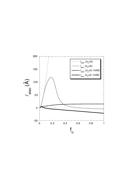
Figure 1: The electrostatic persistence length $\ell_{elec}$ (the solid lines) as a function of $f_{0}$ (the fraction of charged monomers). We have chosen the parameters $b=1.7{\rm\AA}$, $\ell_{B}=7.1{\rm\AA}$, and $n_{1}=1{\rm mM}$. Due to the competition between the net charge repulsion and charge correlations, $\ell_{elec}$ does not vary monotonically. In the absence of multivalent ions $(n_{2}=0)$, $\ell_{elec}$ grows monotonically with $f_{0}$ up to $f_{0}=0.2$, consistent with OSF result (the thin dotted line). Beyond this, however, charge correlations become important and tend to shrink the persistence length. In the presence of a small concentration of 0.1mM of trivalent counterions ($Z=3$), charge correlation effects are dominant and tend to reduce $\ell_{elec}$ beyond $f_{0}\simeq 0.05$. Over a wide range of $f_{0}$ ($f_{0}>0.1$), $\ell_{elec}$ is negative. Due to preferential adsorption of multivalent counterions, even OSF result (the thick dotted line) deviates significantly from the corresponding monovalent case (the thin-dotted line)

The effect of counterion condensation is far more pronounced in the presence of a small concentration of 0.1mM of trivalent counterions ($Z=3$). Both OSF result (the bold dotted line) and our result (the bold solid line) start to deviate from the monovalent case (corresponding to the thin curves) beyond $f_{0}\simeq 0.05$. In other words, the presence of 0.1mM of trivalent counterions is more influential on the bending rigidity of PE chains than that of 1mM of monovalent ions. The result for $\ell_{elec}$ in this case is strikingly different from the corresponding monovalent case; $\ell_{elec}$ is much smaller than in the corresponding monovalent case as long as $f_{0}>0.05$; it is also negative over a wider range of $f_{0}$. Our results clearly demonstrate the efficiency of multivalent counterions in shorterning the persistence length of the PE chain, thus causing the collapse of the PE chain. The efficiency of $Z=3$ in reducing $\ell_{elec}$ can be attributed to the interplay between preferential adsorption of multivalent counterions (over monovalent ones) and charge fluctuation effects in determining the persistence length; highly charged macrions can preferentially bind multivalent counterions even when the bulk concentration is dominated by monovalent ions. Thus multivalent counterions are far more efficient on a molar basis in neutralizing the macroion charge jacob . The OSF result in the presence of a tiny concentration of multivalent counterions can strongly deviate from that for monovalent cases. Additionally, the strength of charge fluctuations grows approximately linearly with the valency of counterions, if preferential adsorption is assumed. When these two effects are combined, multivalent counterions can dramatically change the bending rigidity of PE chains as demonstrated in Fig. 1.

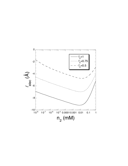
Figure 2: The electrostatic persistence length (described by the solid line) as a function of $n_{2}$ (the concentration of $Z$-valent counterions) for $b=1.7\AA$, $\ell_{B}=7.1\AA$, $n_{1}=1{\rm mM}$, and $Z=3$ (trivalent salts). The persistence length $\ell_{elec}$ varies non-monotonically with $n_{2}$ for the all cases of $f_{0}=1,0.75,0.5$ and takes on a minimum at a certain value of $n_{2}$ in the range $0.01{\rm mM}<n_{2}<0.1{\rm mM}$; only a small concentration is needed to soften PEs. The efficiency of trivalent counterions in softening the PE chain arises from the interplay between preferential adsorption of multivalent counterions and charge fluctuations in determining $\ell_{elec}$. Also note that there is an optimal value of $n_{2}$ at which $\ell_{elec}$ has the minimum value. At zero concentration of PE chains as in this figure, only a tiny concentration of multivalent counterions is needed to almost completely neutralize the backbone charges of the PE chain. Beyond the optimal value, multivalent ions start to contribute toward screening the charge correlation effect, leading to the non-monotonic variation of $\ell_{elec}$ with $n_{2}$.

To further demonstrate the dramatic effects of multivalent counterions, we have estimated the electrostatic persistence length as a function of the concentration of multivalent counterions $n_{2}$. We have chosen the parameters $Z=3$, $n_{1}=1{\rm mM}$, $b=1.7{\rm\AA}$, $r_{c}=2{\rm\AA}$, and $\ell_{B}=7.1{\rm\AA}$. We plot the electrostatic persistence length $\ell_{elec}$ in Fig. 2 as a function of $n_{2}$ for a few different values of $f_{0}$. Our results in the figure are intriguing. For all these cases (ı.e., $f_{0}=1,0.75,0.5$), $\ell_{elec}$ varies non-monotonically with $n_{2}$. It becomes more negative as $n_{2}$ increases from zero up to a certain value of $n_{2}$. Beyond this, it decreases in magnitude with increasing $n_{2}$. This implies that there is an optimal concentration at which $\ell_{elec}$ is most negative. Somehow this optimal value is not sensitive to $f_{0}$; it falls in the range $0.01{\rm mM}\leq n_{2}\leq 0.1{\rm mM}$ and hence only a small concentration is needed to soften PE chains. This clearly demonstrates the efficiency of multivalent counterions in softening oppositely charged PE chains. For the entire range of $n_{2}$ adopted in Fig. 2, $\ell_{elec}$ does not show a simple scaling law. When $n_{2}$ is somewhat smaller than the optimal value, $\ell_{elec}$ has weak dependence on $n_{2}$ as shown in the figure. We find that, for all cases (ı.e., $f_{0}=1,0.75,0.5$), $\ell_{elec}$ assumes the simple scaling form: $\ell_{elec}\sim c+d\log n_{2}$, where $c$ and $d$ are $n_{2}$-independent negative numbers and the concentration $n_{2}$ is in mM. As evidenced in Fig. 2, $d$ (ı.e., the slope of the curves) is insensitive to $f_{0}$; it has been estimated to be close to $-0.2{\rm\AA}$ for all three cases. In contrast, $c$ changes linearly with $f_{0}$ and is more negative for larger $f_{0}$; for the chosen parameters, $c$ has shown to be approximately given by $c\approx-10f_{0}$ (Å). It should be emphasized that both $c$ and $d$ are non-universal constants that can depend on $\kappa$ and $Z$ for fixed $\ell_{B}$ and $b$. Also note that this simple scaling behavior can be invalidated by the competitive binding on the one hand and the presence of the opposing effects in determining $\ell_{elec}$ (cf. eq 11) on the other.

The efficiency of multivalent counterions as evidenced by our results in Fig. 2 can also be understood in terms of competitive binding and charge fluctuations. When $n_{2}=0$, only the monovalent counterions bind to the PE chain. When $n_{2}\neq 0$, however, the PE chain can preferentially bind multivalent counterions, replacing monovalent counterions in its vicinity, thus softening the PE chain, as can be seen by solving the linear equations in eq 13 simultaneously remark1 . For sufficiently highly charged PE chains $(f_{0}\simeq 1)$ at zero concentration, only a tiny concentration of multivalent counterions is needed to replace monovalent counterions. Note that the optimal value of $n_{2}$ at which $\ell_{elec}$ has the minimum value depends not only on $n_{1}$ but also on the concentration of PE chains. Beyond the optimal value, multivalent counterions start to contribute toward screening, weakening the correlation effect and thus leading to the non-monotonic variation of $\ell_{elec}$ with $n_{2}$. Our result in Fig. 2 corresponds to PE chains at zero concentration and thus a direct comparison of our result to experimantal data for PE chains at non-zero concentration should be made with due caution. Finally, computer simulations have explicitly provided evidence for the efficiency of multivalent counterions in inducing collapse of strongly charged polyelectrolytes Lee .

II.3 Multi-loops

So far we have restricted ourselves to the single-loop case. Due to the breakdown of the pairwise additivity of charge-fluctuation interactions ha.bundle ; ha.pre , it is important to discuss the effects of inter-loop coupling on the bending rigidity. Based on our common intuition, we expect the inter-loop interactions to stiffen the condensate. This is because the net charge repulsion is longer ranged than the attraction ha.2rods . This conjecture is, however, based on the pairwise additivity of the electrostatic interactions between different loops and can easily be invalidated unless the charge fluctuations are small enough ha.bundle ; ha.pre ; ha.interface . For the case of parallel rods, it has been shown that the pairwise additivity is valid only when the interaction is repulsive ha.bundle ; ha.pre . By the same token, it is crucial to include non-pairwise additive interactions or many-body effects thirum in the description of the bending rigidity of PE condensates. Because the solution of eq 10 in general cases is difficult, we invoke physically motivated simplification. To understand the physical consequences of non-pairwise additive interactions on the bending rigidity, we make some approximations. First we do not explicitely include excluded volume repulsion between loops. To keep different loops from approaching arbitrarily close to each other, we assume that loops in the condensate are arranged on a square lattice with lattice constant $a$. The lattice constant $a$ can be considered as an equilibrium distance between two neighboring loops, which is determined by the balance of a few competing effects: charge correlation attractions, excluded volume repulsions, etc. We also assume that all loops in the bundle remain parallel with each other, even when they bend, and that $\bar{\Delta}_{j}$ and $\bar{q}_{j}$ are independent of $j$ and taken to be equal to $\bar{\Delta}$ and $\bar{q}$, respectively. With this simplification, we can take advantage of this periodicity to recast the problem using discrete Fourier transform. The resulting bending free energy is given by

$$\ell_{elec} \simeq {\bar{q}^{2}\,\left({}^{0}\!\tilde{D}\right)\over\left[1+2\xi\bar{\Delta}\,\left({}^{0}\tilde{K_{0}}\right)\right]^{2}}-\sum_{j_{1}j_{2}=0}^{\sqrt{N}-1}\int dsD_{{\bf j}_{\bot}}(s)$$ (15)

$$\times\sum_{{\bf k}_{\bot}}\int{dk\over 2\pi}{2\bar{\Delta}\xi\tilde{K_{0}}({\bf k}_{\bot},k)\over 1+2\bar{\Delta}\xi\tilde{K_{0}}({\bf k}_{\bot},k)}\cos({\bf k}_{\bot}\cdot{\bf j}_{\bot})$$

$$\times\cos ks,$$

where ${\bf k}_{\bot}$ is the wave vector conjugate to $a{\bf j}_{\bot}$, where ${\bf j}_{\bot}\equiv(j_{1},j_{2})$ and $j_{1},j_{2}=0.1,\ldots,\sqrt{N}-1$, and is given by ${\bf k}_{\bot}={2\pi\over\sqrt{N}}(n_{1},n_{2})$ with $n_{1},n_{2}=0,1,\ldots,\sqrt{N}-1$. We denote the discrete Fourier transform of a function $g(a|{\bf j}_{\bot}|\sqrt{\kappa^{2}+k^{2}})$ as

$$\tilde{g}(k,{\bf k}_{\bot})\equiv\sum_{j_{1}j_{2}=0}^{\sqrt{N}-1}g(a|{\bf j}_{\bot}|\sqrt{\kappa^{2}+k^{2}})\cos{\bf k}_{\bot}\cdot{\bf j}_{\bot}.$$ (16)

Finally, the function ${}^{0}\tilde{g}$ is simply $g(k=0,{\bf k}_{\bot}=0)$.

First note that the bending free energy of $N$-loop condensates is not simply $N$ times that of a single loop. Our theory suggests that each loop in a bundle is further softened due to the inter-loop coupling, as implied by eq 15. We expect that the repulsive bending rigidity per loop $decreases$ with $N$. This is because coupling between charges on different loops enhances screening in electrostatic repulsions. Similarly, the attractive interaction becomes stronger as $N$ increases, due to enhanced charge correlations as will be detailed later. More precisely, inter-loop correlations enhance intra-loop correlations. A similar issue for the case of rigid PEs is discussed by Ha and Liu ha.correlation . The implication of eq 15 is most striking in the limit of $\kappa b\rightarrow 0$: For sufficiently large $N$, the repulsive term in eq 15 scales as $1/N$ and becomes vanishingly small as $N\rightarrow\infty$. Thus, only the attraction can modify the bending rigidity in this case. Recently, Ha and Liu ha.interface have considered two interacting bundles of randomly-charged rods and shown that, as $\kappa b\rightarrow 0$, the interfacial interaction comes from charge-fluctuation attractions only. This is analogous to the vanishingly small contribution of the repulsion to the bending rigidity in the present case. For the screened case of $\kappa\neq 0$, on the other hand, the repulsion also contributes to the bending rigidity.

For sufficiently large $N$, we can show that the condensate has a well-defined bulk bending free energy: $\Delta{\cal F}_{\rm elec}\sim V\ell_{bulk}$ where $V$ is the condensate volume and $\ell_{bulk}$ is $N$-independent persistence length. To establish this, we examine the behavior of ${}^{0}K_{0},\tilde{K_{0}}(k,{\bf k}_{\bot})$, and $\tilde{D}(k,{\bf k}_{\bot})$ for large $N$. For large $x$, $K_{0}(x)\sim 1/\sqrt{x}{\rm e}^{-x}$ and thus ${}^{0}\tilde{K_{0}},{}^{0}\tilde{D},\tilde{K_{0}}(k,{\bf k}_{\bot})$ approach constants as $N\rightarrow\infty$. Similarly, it can be shown that ${}^{0}\tilde{D},\tilde{D}(k,{\bf k}_{\bot})$ also become constants as $N\rightarrow\infty$. This is trivially true for finite $\kappa$. As $\kappa\rightarrow 0$, it suffices to establish this asymptotic behavior for the attractive term only, since the repulsive term becomes dominated in this limit. As $\kappa\rightarrow 0$, $D_{ij}(s)$ in eq II.1 vanishes at least as fast as $1/R_{ij}^{2}$ for large $|i-j|$. Thus the descrete Fourier transform is convergent. Furthermore, for large $N$, we can replace the sum $\sum_{{\bf k}_{\bot}}$ can be replaced by $N\int_{0}^{2\pi/a}{d{\bf k}_{\bot}\over(2\pi)^{2}}$, up to a correction of order unity. From these arguments, we conclude that the bending free enegy per monomer increases linearly with $N$ for sufficiently large $N$. This enables us to write the total bending free energy as $\Delta{F}_{elec}/k_{B}T={1\over 2}\ell_{bulk}V/R^{2}a^{2}$, where $\ell_{bulk}$ is $N$-independent persistence length per loop. An asymptotic behavor of $\ell_{bulk}$ can be obtained replacing the summations by integrals; we found that, for $\kappa D\ll 1$, $\ell_{bulk}$ varies as

$$\ell_{bulk}\sim-{\kappa^{-1}\over\log(\kappa^{-1}/D)},$$ (17)

where $D$ is the crosssectional diameter of the bundle, $D=\sqrt{N}a$. This should be compared with the corresponding result for a single loop case; the PE chains are further softened by inter-loop couplings by the factor of $\log(b/D)$. Park et al. park have used a similar expression for the bending free energy (Cf. their eq 1) without the benefit of derivation. Here, we have shown that “many-body effects”, ı.e., loop-loop couplings, lead to the bending free energy of PE condensates which grows linearly with $N$ for $N\gg 1$, providing a quantitative basis for the previous work of Park et al. park .

III Conclusions

In conclusion, we have studied the effect of charge fluctuations on the stiffness of highly charged stiff PE chains. In particular, we have focused on the interplay between competitive binding of counterions to PE chains and charge correlations between condensed counterions in softening the PE chains. We have shown that the bending rigidity of the PE chain, in the presence of counterion condensation, cannot be captured by a simple scaling behavior. The existence of multiple distinct regimes characterizes the conformations of highly charged PEs. This is a consequence of the simultaneous presence of competing interactions, which tends to invalidate a simple scaling analysis. Our theory also illustrates the significance of non-pairwise additivity of counterion-mediated interactions in softening PE chains; we have shown that the inter-loop coupling enhances softening, resulting in a well-defined bulk bending free energy.

Acknowledgements: This work was supported in part by the National Science Foundations through grant number CHE0209340 (DT) and by the Natural Science and Engineering Research Council of Canada (BYH). We are grateful to D. Andelmann for helpful comments.

Appendix A

In this appendix we argure that the Debye-Hückel (DH) approach may be valid over a much wider parameter space than implied by a simple thermodynamic consideration in Ref. nguyen . In Ref. nguyen , condensed counterions are considered as forming a strongly correlated liquid (SCL) confined to the surface of their binding PE chains. It was then argued that the negative, charge correlation contribution to the persistence length is dominated by these strong charged correlations of the SCL. In this appendix, we argue the thermodynamic argument underestimates the importance of long-wavelength charge fluctuations as compared to SCL correlations, since it ignores the coupling of charge correlations to bending. Recently, it has been shown that, at high temperatures, long-wavelength (LW) charge fluctuations dominate the free energy, while short-wavelength (SW) fluctuations are dominant at low temperatures ha.mode . Even below the freezing temperature, there exists a LW contribution to the free energy. Interestingly the major contribution to the electrostatic bending rigidity of a polyelectrolyte chain can arise from LW charge fluctuations even when the free energy is dominated by SW fluctuations, as long as the chain is near the rod limit. This is because small bending is more effectively felt by the LW charge fluctuations. In this case the DH approach ought to be a good approximation.

To focus on the essential physics of this issue, we here consider a single-loop case where all backbone charges are neutralized by counterions. Near the rod limit, we can write the interaction Hamiltonian as follows: ${\cal H}={\cal H}_{\rm rod}+\Delta{\cal H}$ where ${\cal H}_{\rm rod}$ corresponds to the rodlike conformation and $\Delta{\cal H}$ is the change in the interaction due to bending. The free energy cost due to bending is

$$\Delta{\cal F}=\left<\Delta{\cal H}\right>={1\over 2}\sum_{ss^{\prime}}D(s,s^{\prime})\left<q(s)q(s^{\prime})\right>+{\cal O}\left(R^{-4}\right),$$

where $\left<\cdots\right>$ is an average with respect to the Boltzmann factor ${\rm e}^{-{\cal H}_{\rm rod}/k_{B}T}$ and $D(s,s^{\prime})$ is

$$D(s,s^{\prime})={\xi\over 24}{{\rm e}^{-\kappa|s-s^{\prime}|}\over|s-s^{\prime}|}\left(|s-s^{\prime}|^{2}+\kappa|s-s^{\prime}|^{3}\right).$$

The charge correlation contribution to the persistence length can be read off from this expression:

$$\ell_{corr}={\xi\over 24L}\sum_{ss^{\prime}}D(s,s^{\prime})\left<q(s)q(s^{\prime})\right>.$$

Now the computation of the persistence length reduces to the computation of the charge correlation function $\left<q(s)q(s^{\prime})\right>$. So far our formalism is exact up to $1/R^{2}$.

If we use a Debye-Hückel (DH) approximation, then $\left<q(s)q(s^{\prime})\right>$ is simply

$$\left<q(s)q(s^{\prime})\right>_{DH}=Q^{-1}(s,s^{\prime}),$$

where $Q$ is a matrix whose matrix element $Q(s,s^{\prime})$ is

$$Q(s,s^{\prime})=\bar{\Delta}^{-1}\delta_{ss^{\prime}}+\ell_{B}{{\rm e}^{-\kappa|s-s^{\prime}|}\over|s-s^{\prime}|}.$$

As a result, the persistence length in eq $A3$ reduces to the one in eq 12. In the limit of $\kappa\rightarrow 0$, the DH approximation leads to

$$\ell_{DH}\simeq-{\left(\xi\bar{\Delta}\right)^{2}\over 16}{\kappa^{-1}\over 1+2\xi\bar{\Delta}\log(1/\kappa b)}.$$

The persistence length in this expression grows linearly with the Debye screening length.

At low temperatures, the backbone charges together with the condensed counterions tend to be strongly correlated. To simplify the problem we assume that $f_{0}=1$ and that counterions are divalent ($Z=2$) and form an ionic crystal such that the charge distribution along the chain is represented by a ground state $(+-+-+-+-)$. The resulting charge correlation can then be approximated by the following oscillatory function: $\left<q(s)q(s^{\prime})\right>_{osc}\simeq\cos(\pi|s-s^{\prime}|/b)$. If we use this expression in eq $A3$, then we have

$$\ell_{osc}={\xi\over 6}\sum_{s=1}^{\infty}{{\rm e}^{-\kappa s}\over s}\left(s^{2}+\kappa s^{3}\right)\cos\left({\pi s\over b}\right).$$

In the limit of $\kappa b\rightarrow 0$, $\ell_{osc}$ approaches

$$\ell_{osc}=-{\ell_{B}\over 26}.$$

This result can be compared to the one based on the SCL model of polyelectolytes nguyen , $\ell_{SCL}=-Z^{2}\ell_{B}/96$. For $Z=2$, this leads to $\ell_{SCL}=-\ell_{B}/24$. Note that $\ell_{SCL}$ is only slightly different from the one in eq $A8$. This difference can be attributed to the fact that we treat the charge fluctuations differently from the SCL approach. Note that $\ell_{DH}$ is much larger than $\ell_{SCL}$ for small $\kappa b$. This is becase the LW charge fluctuations are much more effectively felt by small bending in this case.

However, neither of $\ell_{DH}$ nor $\ell_{OSC}$ solely describes the bending rigidity of polyelectrolyte chains for a wide range of $T$ or $f_{0}$. This is because $\ell_{OSC}$ suppresses fluctuations while $\ell_{DH}$ does not accurately capture strong charge fluctuations. In general both LW and SW charge flcutuations contribute to the persistence length. To study the competition between the two, we use a linear response theory and assume that the free energy of the charge fluctuations on a rod can be written in the Fourier space as

$${{\cal H}_{\rm rod}\over k_{B}T}={1\over 2}\sum_{k}\delta q(k)S^{-1}(k)\delta q(-k),$$

where $S(k)$ is the charge structure factor. The probability of the fluctuation $\delta q(k)$ is proportional to the factor $\exp\left[-S^{-1}(k)\right]$. At high temperatures, $S(k)\equiv S_{DH}(k)\simeq Q^{-1}(k)$ while at low temperatures $S(k)\equiv S_{OSC}(k)\simeq\delta_{k\,{\pi\over b}}$. At intermediate temperatures, we assume that $S(k)\sim A(T)S_{DH}(k)+B(T)S_{OSC}(k)$. Within this approximation, the charge correlation persistence length is given by

$$\begin{aligned} \ell_{corr}\sim&-A(T)\ell_{DH}-B(T)\ell_{OSC}\\ \sim&-A(T){\xi\bar{\Delta}\over 32}{\kappa^{-1}\over\log(1/\kappa b)}-B(T){\ell_{B}\over 26}\end{aligned}.$$

Suppose the free energy is dominated by short-wavelength fluctuations, ı.e., $A(T)\ll B(T)$. Even in this case, however, the persistence length can be dominated by long-wavelength fluctuations, ı.e., $\ell_{corr}\sim A(T)\ell_{DH}$ in the limit of $\kappa b\rightarrow 0$. This is because small bending is much more effectively felt by the long-wavelength fluctuations in this limit. Unfortunately, the precise form of $A(T)$ and $B(T)$ for a wide range of $T$ are not known to date. Nevertheless it is clear that $A(T)\approx 1$ is a good approximation at high temperatures, while $B(T)\rightarrow 1$ as $T\rightarrow 0$. Near and at the crossover region between $\ell_{DH}$ and $\ell_{OSC}$, however, $A(T)$ and $B(T)$ may deviate from this asymptotic value, ı.e., 1. If we use this, we would get a simple criterion for the DH approach to be valid:

$${\kappa^{-1}\over\log\left(1/\kappa b\right)}>1.$$

Note that this can easily be satisfied at a low salt limit. This implies that the electrostatic persistence length can be mainly determined by $\ell_{DH}$, even when $A(T)\approx B(T)$. As a result, our DH approach is valid for a much wider parameter space than implied by Ref. nguyen which suppressed the interplay between chain deformation and charge correlations in determining the mode of charge correlations that dominates the persistence length.

IV Appendix B

In this appendix, we outline the derivation of our major result in eq 10. In this appendix we use $D$ to denote $\mbox{\boldmath$Q$}-\mbox{\boldmath$Q_{0}$}$. First consider the first term of eq 10. To simplify this term, consider

$$\begin{aligned} I&\equiv\sum_{ss^{\prime}}\left[\mbox{\boldmath$Q$}_{0}^{-1}\mbox{\boldmath$D$}\mbox{\boldmath$Q$}_{0}^{-1}\right]_{jj^{\prime}ss^{\prime}}\\ &=\sum_{ss^{\prime}s^{\prime\prime}s^{\prime\prime\prime}}\left[{\left(\mbox{\boldmath$Q$}_{0}^{-1}\right)}_{ss^{\prime\prime}}\mbox{\boldmath$D$}_{s^{\prime\prime}s^{\prime\prime\prime}}{\left(\mbox{\boldmath$Q$}_{0}^{-1}\right)}_{s^{\prime\prime\prime}s^{\prime}}\right]_{jj^{\prime}}\end{aligned}.$$

In this equation and in what follows, $\left(\mbox{\boldmath$A$}_{ss^{\prime}}\right)_{jj^{\prime}}=\mbox{\boldmath$A$}_{ss^{\prime}jj^{\prime}}$, where $A$ is a block matrix such as $Q$. It then follows that $\left[\left(\mbox{\boldmath$A$}\mbox{\boldmath$B$}\right)_{ss^{\prime}}\right]_{jj^{\prime}}=\left(\sum_{s^{\prime\prime}}\mbox{\boldmath$A$}_{ss^{\prime\prime}}\mbox{\boldmath$B$}_{s^{\prime\prime}s^{\prime}}\right)_{jj^{\prime}}=\sum_{j^{\prime\prime}}\sum_{s^{\prime\prime}}\mbox{\boldmath$A$}_{jj^{\prime\prime}ss^{\prime\prime}}\mbox{\boldmath$B$}_{j^{\prime\prime}j^{\prime}s^{\prime\prime}s^{\prime}}$, where $B$ is also a block matrix of the same rank. Note that $\left(\mbox{\boldmath$Q$}_{0}^{-1}\right)_{jj^{\prime\prime}ss^{\prime\prime}}$ is a function of $|s-s^{\prime\prime}|$. It is easy to show that

$$\sum_{s}\left(\mbox{\boldmath$Q$}_{0}^{-1}\right)_{jj^{\prime\prime}ss^{\prime\prime}}=\left[\sum_{s}\left(\mbox{\boldmath$Q$}_{0}^{-1}\right)_{ss^{\prime\prime}}\right]_{jj^{\prime\prime}}={}^{0}\!{\cal M}^{-1}_{jj^{\prime\prime}},$$

where ${}^{0}\!{\cal M}$ is the same matrix defined in eq 8. Here, the second step follows from

$$\begin{aligned} \left[\sum_{s}\left(\mbox{\boldmath$Q$}_{0}^{-1}\right)_{ss^{\prime\prime}}\right]_{jj^{\prime\prime}}&=\left[\sum_{s}\left({1\over\bar{\Delta}^{-1}+\mbox{\boldmath$V$}}\right)_{ss^{\prime\prime}}\right]_{jj^{\prime\prime}}\\ &=\left[\sum_{s}\bar{\Delta}\left(1-\bar{\Delta}\mbox{\boldmath$V$}+\bar{\Delta}^{2}\mbox{\boldmath$V$}^{2}+...\right)_{ss^{\prime\prime}}\right]_{jj^{\prime\prime}}\\ &={1\over b}\left[\bar{\Delta}\left(1-\bar{\Delta}2\xi K_{0}+\Delta^{2}(2\xi K_{0})^{2}+...\right)\right]_{jj^{\prime\prime}}\\ &={}^{0}\!{\cal M}^{-1}_{jj^{\prime\prime}}\end{aligned},$$

where $\mbox{\boldmath$V$}_{jj^{\prime}ss^{\prime}}=\ell_{B}{e^{-\kappa|{\bf r}_{j}(s)-{\bf r}_{j^{\prime}}(s^{\prime})|}\over|{\bf r}_{j}(s)-{\bf r}_{j^{\prime}}(s^{\prime})|}$ and $\left(K_{0}\right)_{jj^{\prime}}=K_{0}(\kappa R_{jj^{\prime}})$. If we use this in eq $B1$, then we have

$$I=\left[{}^{0}\!{\cal M}^{-1}\sum_{s^{\prime\prime}s^{\prime\prime\prime}}\mbox{\boldmath$D$}_{s^{\prime\prime}s^{\prime\prime\prime}}{}^{0}\!{\cal M}^{-1}\right]_{jj^{\prime}}.$$

This , if combined with eq 6, essentially leads to the first term of eq 10 in the continuum limit.

To simplify the second term of eq 10, consider

$$J\equiv\left(\mbox{\boldmath$Q$}_{0}^{-1}\mbox{\boldmath$D$}\right)_{jjss}=\left[\sum_{s^{\prime}}\left(\mbox{\boldmath$Q$}_{0}^{-1}\right)_{ss^{\prime}}\mbox{\boldmath$D$}_{s^{\prime}s}\right]_{jj}.$$

Here $\left(\mbox{\boldmath$Q$}_{0}^{-1}\right)_{ss^{\prime}}$ can be expanded as follows:

$$\begin{aligned} \left(\mbox{\boldmath$Q$}_{0}^{-1}\right)_{ss^{\prime}}&=\left({1\over\bar{\Delta}_{j}^{-1}+\mbox{\boldmath$V$}}\right)_{ss^{\prime}}\\ &=\bar{\Delta}_{j}\bigg{(}\delta_{ss^{\prime}}-\bar{\Delta}_{j}\mbox{\boldmath$V$}_{ss^{\prime}}+\bar{\Delta}_{j}^{2}\sum_{s^{\prime\prime}}\mbox{\boldmath$V$}_{ss^{\prime\prime}}\mbox{\boldmath$V$}_{s^{\prime\prime}s^{\prime}}+...\bigg{)}\end{aligned}.$$

Using this in eq $B5$, we have

$$\begin{aligned} J=&\bar{\Delta}_{j}\bigg{[}\mbox{\boldmath$D$}_{ss}-\sum_{s^{\prime}}\bigg{(}\bar{\Delta}_{j}\mbox{\boldmath$V$}_{ss^{\prime}}\mbox{\boldmath$D$}_{ss^{\prime}}\\ &-\bar{\Delta}_{j}^{2}\sum_{s^{\prime}s^{\prime\prime}}\mbox{\boldmath$V$}_{ss^{\prime\prime}}\mbox{\boldmath$V$}_{s^{\prime\prime}s^{\prime}}\mbox{\boldmath$D$}_{s^{\prime}s}\\ &+\bar{\Delta}_{j}^{3}\sum_{s^{\prime}s^{\prime\prime}s^{\prime\prime\prime}}\mbox{\boldmath$V$}_{ss^{\prime\prime}}\mbox{\boldmath$V$}_{s^{\prime\prime}s^{\prime\prime\prime}}\mbox{\boldmath$V$}_{s^{\prime\prime\prime}s^{\prime}}\mbox{\boldmath$D$}_{s^{\prime}s}+...\bigg{)}\bigg{]}_{jj}\end{aligned}.$$

Note that the first-order term in $\bar{\Delta}_{j}$ in this equation will cancel the term containing $\bar{\Delta}$ in the second term of eq 10. As a result, the second term of eq 10 becomes

$$\begin{aligned} \mbox{2nd term}&=-{1\over 2}\sum_{j}\bar{\Delta}_{j}\bigg{[}\sum_{ss^{\prime}}\bigg{(}\bar{\Delta}_{j}\mbox{\boldmath$V$}_{ss^{\prime}}\mbox{\boldmath$D$}_{ss^{\prime}}\\ &-\bar{\Delta}_{j}^{2}\sum_{s^{\prime\prime}}\mbox{\boldmath$V$}_{ss^{\prime\prime}}\mbox{\boldmath$V$}_{s^{\prime\prime}s^{\prime}}\mbox{\boldmath$D$}_{s^{\prime}s}\\ &+\bar{\Delta}_{j}^{3}\sum_{s^{\prime\prime}s^{\prime\prime\prime}}\mbox{\boldmath$V$}_{ss^{\prime\prime}}\mbox{\boldmath$V$}_{s^{\prime\prime}s^{\prime\prime\prime}}\mbox{\boldmath$V$}_{s^{\prime\prime\prime}s^{\prime}}\mbox{\boldmath$D$}_{s^{\prime}s}+...\bigg{)}\bigg{]}_{jj}\end{aligned}.$$

In the Fourier space $k$, conjugate to $s-s^{\prime}$, this equation can be diagonalized with respect to $s$ and $s^{\prime}$ and resummed:

$$\begin{aligned} \mbox{2nd term}=&-{M\over 2}\sum_{j}\bar{\Delta}_{j}\bigg{[}\int{dk\over 2\pi}\bigg{(}\bar{\Delta}_{j}\mbox{\boldmath$V$}(k)\mbox{\boldmath$D$}(k)\\ &-\bar{\Delta}_{j}^{2}\mbox{\boldmath$V$}(k)\mbox{\boldmath$V$}(k)\mbox{\boldmath$D$}(k)\\ &+\bar{\Delta}_{j}^{3}\mbox{\boldmath$V$}(k)\mbox{\boldmath$V$}(k)\mbox{\boldmath$V$}(k)\mbox{\boldmath$D$}(k)+...\bigg{)}\bigg{]}_{jj^{\prime}}\\ &=-{M\over 2}\sum_{j}\bar{\Delta}_{j}\bigg{[}\int{dk\over 2\pi}{\bar{\Delta}_{j}\mbox{\boldmath$V$}(k)\mbox{\boldmath$D$}(k)\over 1+\bar{\Delta}_{j}\mbox{\boldmath$V$}(k)}\bigg{]}_{jj}\end{aligned},$$

where $f(k)$ is a Fourier transform of $f(s)$: $f(k)=\sum_{s}f(s)\cos ks$. This essentially leads to the second term of eq 10.

References

- (1) Bloomfield, V. A. Biopolymers 1991, 31, 1471.
- (2) Steven, M. J.; Kremer, K. J. Chem. Phys. 1995, 103, 5781.
- (3) Winkler, R. G.; Gold, M.; Reineker, P. Phys. Rev. Lett. 1998, 80, 3731.
- (4) Shiessel, H.; Pincus, P. Macromolecules 1998, 31, 7959.
- (5) See Tang, J. X.; Wong, S.; Tran, P.; Janmey, P. Ber. Buns. Phys. Chem. 1996, 100, 1, and references therein.
- (6) See also Tang, J.X.; Ito, T.; Tao, T.; Traub, P.; Janmey, P.A. Biochemistry 1997, 36, 12600, and references therein.
- (7) Sedlák, M.; Amis, E.J. J. Chem. Phys. 1992, 96, 817; J. Chem. Phys. 1992, 96, 826.
- (8) Brilliatov, N. V.; Kuznetsov, D.V.; Klein, R. Phys. Rev. Lett. 1998, 81, 1433.
- (9) Ha, B.-Y.; Liu, A.J. Phys. Rev. Lett. 1997 79, 1289.
- (10) Ha, B.-Y.; Liu, A.J. Phys. Rev. Lett. 1998 81, 1011.
- (11) Ha, B.-Y.; Liu, A.J. Phys. Rev. E 1999 60, 803.
- (12) Ha, B.-Y.; Liu, A.J. Europhys. Lett. 1999, 46, 624.
- (13) Lee, N.; Thirumalai, D. Macromolecules 2001, 34, 3446.
- (14) Grønbech-Jensen, N; Mashl, R.J.; Bruinsma, R.F.; and Gelbart, W.M. Phys. Rev. Lett. 1997, 78, 2477.
- (15) See Marcelja, S. Biophys. J. 1992, 61, 1117, and references therein.
- (16) Barrat, J. L.; Joanny, J.F. Advances in Chemical Physics 1996, 94, 1.
- (17) Podgornik, R.; Parsegian, V.A. Phys. Rev Lett. 1998, 80, 1560.
- (18) Oosawa, F. Biopolymers 1968, 6, 134.
- (19) Manning, G. S. J. Chem. Phys. 1969, 51, 954.
- (20) Oosawa, F. Polyelectrolytes 1971 (Marcel Dekker, New York).
- (21) Raspaud, E.; Cruz, M. Olvera de la; Sikorav, J.-L.; Livolant F. Biophys. J. 1998, 74, 381.
- (22) Odijk, T.; Houwaart, A.C. J. Polym. Phys. Ed. 1978, 16, 627; Odijk, T J. Polym. Phys. Ed. 1977, 15, 477; Skolnick, J.; Fixman, M. Macromolecules 1977, 10, 944.
- (23) Park, S.Y.; Harries, D.; Gelbart, W.M. Biophys. J. 1998, 75, 714.
- (24) Ubbink, J.; Odijk, T. Biophys. J. 1995, 68, 54.
- (25) Ha, B.-Y.; Thirumalai, D. J. Phys. (France) 1997, 7, 887.
- (26) Golestanian, R.; Kardar, M; Liverpool, T. Phys. Rev. Lett. 1996, 82, 4456.
- (27) Ariel, G.; Andelman, D. Europhys. Lett. 2003, 61, 67.
- (28) Hansen, P.L.; Svensek, D.; Parsegian, V.A.; Podgornik, R. Phys. Rev. E 1999, 60, 1956.
- (29) Nguyen, T.T; Rouzina, I; Shklovskii, B.I. Phys. Rev. E 1999, 60, 7032.
-
(30)
Note that is related to the
concentration (or number) fluctuations of condensed counterions in chemical
equilibrium with free counterions. First of all, we should
emphasize that the average involved in the estimation of this
qualtity is different from the esemble average denoted by , which is an average
over all realizations of , weighted by the Boltzmann
factor:
In other words, reduces to if the electrostatic interactions among counterions are turned off. In this case, we can consider condensed counterions as forming an ideal gas in chemical contact with free counterions. As a result, charges at different sites are uncorrelated. If and are the total number on loop of monovalent and multivalent counterions, respectively, then it follows from a simple thermodynamic consideration that(18)
where . This gives rise to charge fluctuations along the chain; the total-charge fluctuation of condensed counterions is(19)
where and . This leads to the variance in the charge per site charge used in Sec. II: .(20) - (31) Ha, B.-Y.; Liu, A.J. Physica A 1998 259, 235.
- (32) Note here that the multipole expansion refers to an expansion of the free energy (thus eq 12) in powers of within the one-dimensional Debye-Hückel (DH) approach. Truncation of high order terms in this expansion can be justified only when (thus ) is small enough. In this sense we have summed up the free energy over all realizations of charge fluctuations (within the DH approach). As a result, non-Gaussian fluctuations are suppressed. The validity of this approach is discussed in the appendix, which implies that the DH approach is valid even for large values of as long as is sufficiently small.
- (33) Regarding this equation, it’s worth noting that our approach is somewhat different from the one adopted by Golestanian et al. kardar in the following two respects. We first incorporate the fluctuation correction to the chemical potential of condensed counterions, while the meanfield attraction, ı.e., the first term on the right hand side of our eq 13, is mainly responsible for counterion condensation in Ref. kardar . Second we consider PE solution in the presence of both (1:1) salts and asymmetrical (Z:1) salts, as is the case for a typical biological system. This extra complexity enables us to study the competitive binding between monovalent and multivalent counterions. If we ignored these two complexities, we would have . Our eq 13, when combined with this result, would reproduce the result of Golestanian et al. kardar , ı.e., their eq 2. In the presence of salts, however, becomes important (see Ref. nguyen1 for the detailed discussion). Also the competitive binding will modify this simple scaling law for . To incorporate this, we have solved eq 11 and eq 13 simultaneously.
- (34) For a similar issue for a highly charged surface, see Nguyen, T.T; Grosberg, A.Y; Shklovskii, B.I. Phys. Rev. Lett. 2000, 85, 1568.
- (35) See also Israelachvili J. Intermolecular and Surface Forces, 2nd Ed. 1992 (Academic Press).
- (36) For competitive binding in membrane systems, see Ha, B.-Y. Phys. Rev. E 2003, 67, 30901 (R).
- (37) For many-body effects in non-ionic polymeric solution, see Shaw, M.; Thirumalai, D. Phys. Rev. A 1991, 44, R4797.
- (38) Ha, B.-Y.; Liu, A.J. Phys. Rev. E 1998, 58, 6281.
- (39) Ha, B.-Y. Phys. Rev. E 2001, 64, 31507.