Density functional for anisotropic fluids

Giorgio Cinacchi¹, Friederike Schmid²

1: Dipartimento di Chimica, Universita’ di Pisa, 56126 Pisa, Italy
electronic mail: giorgio@giasone.dcci.unipi.it
2: Fakultät für Physik, Universität Bielefeld, D 33501 Bielefeld, Germany
electronic mail: schmid@physik.uni-bielefeld.de

Abstract

We propose a density functional for anisotropic fluids of hard body particles. It interpolates between the well-established geometrically based Rosenfeld functional for hard spheres and the Onsager functional for elongated rods. We test the new approach by calculating the location of the the nematic-isotropic transition in systems of hard spherocylinders and hard ellipsoids. The results are compared with existing simulation data. Our functional predicts the location of the transition much more accurately than the Onsager functional, and almost as good as the theory by Parsons and Lee. We argue that it might be suited to study inhomogeneous systems.

1 Introduction

The density functional approach is one of the most powerful and widely applicable approaches to nonuniform fluids [1]. Its idea is to express the free energy as a functional of locally varying one-particle densities ${\mathcal{F}}\{\rho({\mathbf{r}})\}$, with an ideal gas contribution and an excess free energy which accounts for the interparticle interactions. This allows one to calculate the structure and properties of fluids with various kinds of inhomogeneities. Density functionals for simple fluids have reached a considerable degree of sophistication and are able to describe such complex phenomena as freezing, wetting, and surface melting [1].

One of the most established density functionals for hard sphere fluids is the Rosenfeld functional [2]. It reproduces by construction the Percus-Yevick solution for the correlation function, which is known to be very good [3]. As a consequence, it provides highly accurate predictions for the structure of inhomogeneous hard sphere fluids [4]. It has been used successfully to study mixtures of hard spheres [5] and polydisperse fluids [6]. After a simple anisotropic mapping procedure it can be applied to fluids of fully aligned ellipsoids [7]. Exploiting the Gauss-Bonnet theorem, it has been generalized for isotropic molecular fluids [8]. This generalized functional has been used as a starting point to calculate direct correlation functions of isotropic multicomponent fluids [9]. A Rosenfeld type approach has been developed for mixtures of rods and needles, assuming that the needles are too thin to interact with each other directly [10], and for systems containing only one single rod immersed in a fluid of spheres [11]. However, to our knowledge, the Rosenfeld functional has not yet been extended to general anisotropic fluids.

The simplest density functional for anisotropic particles is the Onsager functional [12], which truncates the virial expansion after the leading coefficient. Onsager showed that this functional produces a nematic-isotropic phase transition [12] in fluids of sufficiently elongated particles. Its predictions are in good agreement with experimental results on systems of tobacco mosaic viruses [13]. One can even show that it describes the transition exactly in homogeneous systems of infinitely elongated rods [14]. Thus any functional for nematic liquid crystals should reduce to the Onsager functional in this limit.

In the present paper, we propose a density functional for hard anisotropic particles which interpolates between the Rosenfeld functional and the Onsager functional. It reduces to the Rosenfeld functional in the case of particles with spherical symmetry, and to the Onsager functional for homogeneous fluids of infinitely elongated particles at density close to zero. As a first test of the functional, we have calculated the nematic-isotropic transition for hard spherocylinders and hard ellipsoids, and obtained reasonable results. We believe that our functional might provide a useful new approach to the study of inhomogeneous liquid crystals, e.g. the study of interfacial phenomena such as surface anchoring.

2 Background

We consider a fluid of hard anisotropic particles with positions ${\mathbf{r}}$ and orientations $\varpi$. The grand canonical free energy is the minimum of the free energy functional

$$\beta\Omega[\rho]=\beta{\mathcal{F}}^{id}[\rho]+\beta{\mathcal{F}}^{ex}[\rho]+\int d{\mathbf{r}}\>d\varpi\>\rho({\mathbf{r}},\varpi)\>[\mu-V({\mathbf{r}},\varpi)]$$ (1)

with respect to the one-particle density $\rho({\mathbf{r}},\varpi)$, where $\beta=\frac{1}{k_{B}T}$ is the Boltzmann factor with the temperature $T$, $\mu$ the chemical potential and $V({\mathbf{r}},\varpi)$ summarises all external potentials. The first term describes the ideal gas contribution

$$\beta{\mathcal{F}}^{id}=\int d{\mathbf{r}}\>d\varpi\>\rho({\mathbf{r}},\varpi)\>\Big{(}\ln[\rho({\mathbf{r}},\varpi)\lambda_{T}^{3}]-1\Big{)}$$ (2)

with the de Broglie wavelength $\lambda_{T}$. The second term ${\mathcal{F}}^{ex}$ is the excess free energy, the central quantity in density functional theories [1].

In the Onsager theory, the excess free energy of two hard particles is given by

$$\beta{\mathcal{F}}_{O}^{ex}=-\frac{1}{2}\int d{\mathbf{r}}\>d\varpi\>d{\mathbf{r}}^{\prime}\>d\varpi^{\prime}\>\rho({\mathbf{r}},\varpi)\>\rho({\mathbf{r}}^{\prime},\varpi^{\prime})\>\mbox{M}({\mathbf{r}}-{\mathbf{r}}^{\prime},\varpi,\varpi^{\prime}).$$ (3)

The Mayer-function M takes the value $(-1)$ if two particles at $({\mathbf{r}},\varpi)$ and $({\mathbf{r}}^{\prime},\varpi^{\prime})$ overlap and vanishes otherwise. In the homogeneous case, the one-particle density $\rho$ does not depend on ${\mathbf{r}}$ and can be written as $\rho({\mathbf{r}},\varpi)=\rho\>f(\varpi)$. The expression 3 then reduces to

$$\frac{\beta{\mathcal{F}}_{O}^{ex}}{N}=\frac{\rho}{2}\int d\varpi\>d\varpi^{\prime}\>f(\varpi)\>f(\varpi^{\prime})\>\nu(\varpi,\varpi^{\prime}),$$ (4)

where $\nu(\varpi,\varpi^{\prime})$ is the covolume of two particles with orientations $\varpi$ and $\varpi^{\prime}$, and $N$ the total number of particles. Eqn. (4) corresponds to a virial expansion up to second order. As mentioned in the introduction, the Onsager theory is exact in the limit of infinitely elongated particles  [14]. Compared to real thermotropic liquid crystals, it tends to overestimate the shape anisotropy required to observe a nematic phase at a given finite density.

A natural extension of the Onsager model would be to include higher order terms in the virial expansion. On principle, this is feasible, and an extension of the Onsager functional up to third order was actually carried out for ellipsoids  [15]. However , the calculations are very cumbersome due to the increasing complexity of the integrals. As long as one is interested in homogeneous systems, one way to overcome the problem is the decoupling approximation. It consists of a resummation of the virial expansion, where the first virial coefficients are calculated exactly, and the remaining ones are approximated by a mapping onto a reference system. Given a virial expansion of the form:

$$\frac{\beta\mathcal{F}^{ex}}{N}=\sum^{\infty}_{l=1}\frac{\rho^{l}}{l}B_{l+1}\left[f\left(\varpi\right)\right],$$ (5)

the decoupling approximation reads [16]-[19]:

$$\frac{\beta\mathcal{F}^{ex}}{N}=\sum^{r}_{l=1}\frac{\rho^{l}}{l}B_{l+1}\left[f\left(\varpi\right)\right]+\left[\frac{\beta F^{ex,ref}}{N}-\sum^{r}_{l=1}\frac{\rho^{l}}{l}B^{ref}_{l+1}\right]\frac{B_{r+1}\left[f\left(\varpi\right)\right]}{B^{ref}_{r+1}},$$ (6)

where $B_{l+1}\left[f\left(\varpi\right)\right]$ are the virial coefficients of the anisotropic fluids, calculated exactly up to the $r+1$ order and ref refers to the reference system. Two possible reference systems have been proposed: the hard sphere fluid and the isotropic fluid of the particles under investigation. If $r=1$ and the reference system is the hard sphere fluid with the Carnahan-Starling equation of state [20], we recover the Parsons-Lee functional [16, 17]

$$\beta{\mathcal{F}}_{PL}^{ex}=-\frac{1}{8}\frac{(4-3\eta)}{(1-\eta)^{2}}\int d{\mathbf{r}}\>d\varpi\>d{\mathbf{r^{\prime}}}\>d\varpi^{\prime}\>\rho({\mathbf{r}},\varpi)\>\rho({\mathbf{r^{\prime}}},\varpi^{\prime})\>\mbox{M}({\mathbf{r}}-{\mathbf{r^{\prime}}},\varpi,\varpi^{\prime}),$$ (7)

where $\eta$ is the packing fraction. The Parsons-Lee functional predicts accurately the location of the nematic-isotropic phase transition for a wide range of shape anisotropies [21, 22]. It can also be applied to inhomogeneous systems. However, it does not describe the microscopic structure very well: it yields very crude correlation functions [23, 24] and produces rather unrealistic density profiles in inhomogeneous systems as a consequence [25].

The success of the Parsons-Lee theory in predicting the isotropic-nematic coexistence densities motivated Poniewierski and Holyst [26] and Somoza and Tarazona [27] to combine the decoupling approximation with a “weighted density approximation” (WDA) scheme [28, 29, 30]. Both are constructed such that one automatically recovers the Onsager functional in the low density limit. In the hard sphere limit, Somoza’s and Tarazona’s [27] and related [31] versions reduce to the well-known Tarazona functional [29]. The latter incorporates the Carnahan-Starling equation of state and the Percus-Yevick direct correlation function for homogeneous hard sphere fluids, and has been used with great success to study inhomogeneous hard sphere fluids and solids. Applied to systems of spherocylinders, the extensions [27, 31] of the Somoza functional generate a nematic phase and several smectic phases. Graf and Löwen have put forward a simplified “modified weighted density approximation” (MWDA), and used it to reproduce complex phase diagrams of spherocylinder fluids [32].

Besides the Tarazona functional, another equally successful hard sphere functional has established itself in recent years: the fundamental measure theory or Rosenfeld functional [2, 4, 5]. It has the advantage of being based on somewhat more fundamental considerations: it does not require the explicit input of the equation of state and the direct correlation functions, instead they pop out automatically. One obtains by construction the Percus-Yevick solution. Moreover, the functional is formulated a priori for general convex particles of arbitrary geometry. It thus seems to call for a generalization to anisotropic fluids. Unfortunately, there is one problem: the original Rosenfeld functional does not reproduce the Onsager functional in the low density limit.

Here, we propose a simple modification of the Rosenfeld functional which solves that problem for anisotropic particles, and reduces to the original Rosenfeld functional for isotropic particles. Like Somoza’s and Tarazona’s functional, our functional interpolates between an established hard sphere functional and the Onsager functional. Thus we hope that it will be equally useful.

Before introducing our approach, we sketch briefly the basic equations of the original Rosenfeld functional [2]. It can be formulated for general multicomponent fluids of convex hard particles. In our case, different components $i$ may be identified with different particle orientations. The functional then reads:

$$\beta{\mathcal{F}}_{R}^{ex}=\int d{\mathbf{r}}\>\Big{(}\>\Phi_{1}({\mathbf{r}})+\Phi_{2}({\mathbf{r}})+\Phi_{3}({\mathbf{r}})\>\Big{)},$$ (8)

$$\Phi_{1}({\mathbf{r}})=-n_{0}({\mathbf{r}})\ln(1-n_{3}({\mathbf{r}}))$$ (9)

$$\Phi_{2}({\mathbf{r}})=\frac{n_{1}({\mathbf{r}})n_{2}({\mathbf{r}})-{\mathbf{n}}_{1}({\mathbf{r}})\cdot{\mathbf{n}}_{2}({\mathbf{r}})}{1-n_{3}({\mathbf{r}})}$$ (10)

$$\Phi_{3}({\mathbf{r}})=\frac{\frac{1}{3}n_{2}^{3}({\mathbf{r}})-n_{2}({\mathbf{r}})({\mathbf{n}}_{2}({\mathbf{r}})\cdot{\mathbf{n}}_{2}({\mathbf{r}}))}{8\pi(1-n_{3}({\mathbf{r}}))^{2}}\cdot\lambda$$ (11)

The $\Phi$s depend on the weighted densities

$$n_{\alpha}({\mathbf{r}})=\sum_{i}\int d{\mathbf{r}}^{{}^{\prime}}\rho_{i}({\mathbf{r}}^{{}^{\prime}})\>w^{(\alpha)}_{i}({\mathbf{r}}-{\mathbf{r}}^{{}^{\prime}}),$$ (12)

with the number density of the $i$th component $\rho_{i}({\mathbf{r}})$ and the weight functions

$$\begin{array}[]{rcl rcl}w^{(0)}_{i}({\mathbf{r}})&=&C_{i}({\hat{\mathbf{r}}})\>\delta(R_{i}({\hat{\mathbf{r}}})-r)\>K_{i}({\hat{\mathbf{r}}})/4\pi&w^{(2)}_{i}({\mathbf{r}})&=&C_{i}({\hat{\mathbf{r}}})\>\delta(R_{i}({\hat{\mathbf{r}}})-r)\\ w^{(1)}_{i}({\mathbf{r}})&=&C_{i}({\hat{\mathbf{r}}})\>\delta(R_{i}({\hat{\mathbf{r}}})-r)\>H_{i}({\hat{\mathbf{r}}})/4\pi&w^{(3)}_{i}({\mathbf{r}})&=&\Theta(R_{i}({\hat{\mathbf{r}}})-r)\\ {\mathbf{w}}^{(1)}_{i}({\mathbf{r}})&=&C_{i}({\hat{\mathbf{r}}})\>\delta(R_{i}({\hat{\mathbf{r}}})-r)\>{\hat{\mathbf{n}}}_{i}({\hat{\mathbf{r}}})\>H_{i}({\hat{\mathbf{r}}})/4\pi&{\mathbf{w}}^{(2)}_{i}({\mathbf{r}})&=&C_{i}({\hat{\mathbf{r}}})\>\delta(R_{i}({\hat{\mathbf{r}}})-r)\>{\hat{\mathbf{n}}}_{i}({\hat{\mathbf{r}}}).\end{array}$$ (13)

Here ${\hat{\mathbf{r}}}$ denotes the unit vector in the direction of ${\mathbf{r}}$, $R_{i}({\hat{\mathbf{r}}})$ the radius from the centre of a particle of type $i$ to the surface in the direction ${\hat{\mathbf{r}}}$, $H_{i}({\hat{\mathbf{r}}})$ and $K_{i}({\hat{\mathbf{r}}})$ the local mean and Gaussian curvature on that specific surface point [34, 35], ${\hat{\mathbf{n}}}_{i}({\hat{\mathbf{r}}})$ the outward unit normal (see Figure 1), and $\delta$ and $\theta$ are the usual delta and step function. The factor $C_{i}({\hat{\mathbf{r}}})$ ensures that integrals over the weight functions $w^{(\alpha)}_{i}({\mathbf{r}})$ and ${\mathbf{w}}^{(\alpha)}_{i}({\mathbf{r}})$ $(\alpha\neq 3)$ are surface integrals over the surface of the particle $i$. For spherical particles, it can be omitted. In general, it is given by

$$C_{i}({\hat{\mathbf{r}}})=\sqrt{\det\mathbf{g}_{i}({\hat{\mathbf{r}}})/\det\mathbf{g}_{i,\mbox{sph}}({\hat{\mathbf{r}}})},$$ (14)

where $\mathbf{g}_{i}({\hat{\mathbf{r}}})$ is the local metric tensor of the particle $i$, and $\mathbf{g}_{i,\mbox{sph}}({\hat{\mathbf{r}}})$ that of a reference sphere of radius $R_{i}({\hat{\mathbf{r}}})$. (In polar coordinates, $\sqrt{\det\mathbf{g}_{i,\mbox{sph}}({\hat{\mathbf{r}}})}=R_{i}^{2}({\hat{\mathbf{r}}})\sin(\theta)$). Finally, the factor $\lambda$ in Eqn. (11) ensures that the dimensional crossover for hard spheres is reproduced correctly and that the hard sphere system exhibits a solid-fluid transition in three dimensions [4].

$$\lambda=\frac{\left(1-\xi({\mathbf{r}})^{2}\right)^{3}}{1-3\xi({\mathbf{r}})^{2}}\quad\mbox{with}\quad\xi=\left|\frac{{\mathbf{n}}_{2}({\mathbf{r}})}{n_{2}({\mathbf{r}})}\right|.$$ (15)

Alternatively, Eqn. (11) can be replaced by a more modern version due to Tarazona [33], which depends on an additional tensorial weighted density and does not contain the ad hoc factor $\lambda$.

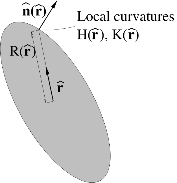
Figure 1: Illustration of $R(\widehat{\mathbf{r}})$ and $\widehat{\mathbf{n}}(\widehat{\mathbf{r}})$.

3 Construction of the functional

As mentioned before, the Rosenfeld functional describes hard sphere fluids very successfully. On principle, it could also be applied to molecular fluids. However, it has the serious drawback that it does not reduce to the Onsager functional in the low density limit. Even worse, a closer inspection of Eqns. (8)–(15) reveals that it has no contribution at all which would favor parallel alignment of particles in a homogeneous fluid. Hence it cannot produce stable homogeneous anisotropic fluids.

The reason for this failure can be understood by looking at the relation between the Mayer-function and the weight functions in more detail. For hard spheres, the Mayer-function for a pair of particles at position ${\mathbf{r}}_{i}$ and ${\mathbf{r}}_{j}$ can be decomposed exactly as [2]

$$-\mbox{M}_{ij}=w_{i}^{(0)}\otimes w_{j}^{(3)}+w_{i}^{(3)}\otimes w_{j}^{(0)}+w_{i}^{(1)}\otimes w_{j}^{(2)}+w_{i}^{(2)}\otimes w_{j}^{(1)}-{\mathbf{w}}_{i}^{(1)}\otimes{\mathbf{w}}_{j}^{(2)}-{\mathbf{w}}_{i}^{(2)}\otimes{\mathbf{w}}_{j}^{(1)},$$ (16)

where $\otimes$ denotes the convolution product:

$$w_{i}^{(\alpha)}\otimes w_{j}^{(\beta)}=\int d{\mathbf{r}}\>w^{(\alpha)}({\mathbf{r}}-{\mathbf{r}}_{i})\>w^{(\beta)}({\mathbf{r}}-{\mathbf{r}}_{j}).$$ (17)

This decomposition together with Eqns. (8)–(12) ensures that the functional reproduces the correct virial expansion at least up to second order. Unfortunately, a decomposition of the type above is no longer valid for anisotropic particles. Therefore, the Onsager limit is not recovered. Chamoux and Perera [9] have proposed ways to cure the virial expansion on the level of the direct correlation function, for the case of isotropic molecular fluids [9]. A systematic way of dealing with the problem on the level of the functional itself would be to add a correction term on the right hand side of Eqn. (16), to deconvolute it (if possible), and then rederive a Rosenfeld type functional on the basis of this new decomposition. This can be done for rod-sphere interactions [11]. An extension to the general case is currently under way [36]. Unfortunately, it turns out that infinitely many additional terms are required in the decomposition in order to make Eqn. (16) exact, and the numerical treatment becomes difficult unless one resorts to approximations.

Here we propose a simpler, numerically perhaps more tractable Ansatz – a straightforward modification of Eqns. (9), (10) and (11). Instead of keeping $n_{1}$ and ${\mathbf{n}}_{1}$ as separate quantities, we suggest to replace the products $n_{1}({\mathbf{r}})n_{2}({\mathbf{r}})$ and ${\mathbf{n}}_{1}({\mathbf{r}})\cdot{\mathbf{n}}_{2}({\mathbf{r}})$ by new joint quantities $n_{12}({\mathbf{r}})$ and $\tilde{n}_{12}({\mathbf{r}})$ such that the functional reproduces correctly the Onsager limit. This is achieved as follows: we define the functions

$$g(\varpi_{i},\varpi_{j},{\mathbf{r}}_{i}-{\mathbf{r}}_{j})\equiv g_{ij} := -M_{ij}-w_{i}^{(0)}\otimes w_{j}^{(3)}-w_{i}^{(3)}\otimes w_{j}^{(0)}$$ (18)

$$h(\varpi_{i},\varpi_{j},{\mathbf{r}}_{i}-{\mathbf{r}}_{j})\equiv h_{ij} := w_{i}^{(1)}\otimes w_{j}^{(2)}+w_{i}^{(2)}\otimes w_{j}^{(1)}-{\mathbf{w}}_{i}^{(1)}\otimes{\mathbf{w}}_{j}^{(2)}-{\mathbf{w}}_{i}^{(2)}\otimes{\mathbf{w}}_{j}^{(1)},$$ (19)

and

$$H^{\mbox{\small eff}}(\varpi_{i},\varpi_{j},{\mathbf{r}}_{i}-{\mathbf{r}}_{j})=g_{ij}/h_{ij}.$$ (20)

Then we replace $n_{1}({\mathbf{r}})n_{2}({\mathbf{r}})$ and ${\mathbf{n}}_{1}({\mathbf{r}})\cdot{\mathbf{n}}_{2}({\mathbf{r}})$ by

$$n_{12}({\mathbf{r}}) := \frac{1}{2}\int\!\!d\varpi_{i}\>d\varpi_{j}\>d{\mathbf{r}}_{i}\>d{\mathbf{r}}_{j}\>\rho({\mathbf{r}}_{i},\varpi_{i})\>\rho({\mathbf{r}}_{j},\varpi_{j})\>H^{\mbox{\small eff}}(\varpi_{i},\varpi_{j},{\mathbf{r}}_{i}-{\mathbf{r}}_{j})$$

$$\times\Big{(}w^{(1)}_{i}({\mathbf{r}}_{i}-{\mathbf{r}})\>w^{(2)}_{j}({\mathbf{r}}_{j}-{\mathbf{r}})+w^{(2)}_{i}({\mathbf{r}}_{i}-{\mathbf{r}})\>w^{(1)}_{j}({\mathbf{r}}_{j}-{\mathbf{r}})\Big{)}$$

$$\tilde{n}_{12}({\mathbf{r}}) := \frac{1}{2}\int\!\!d\varpi_{i}\>d\varpi_{j}\>d{\mathbf{r}}_{i}\>d{\mathbf{r}}_{j}\>\rho({\mathbf{r}}_{i},\varpi_{i})\>\rho({\mathbf{r}}_{j},\varpi_{j})\>H^{\mbox{\small eff}}(\varpi_{i},\varpi_{j},{\mathbf{r}}_{i}-{\mathbf{r}}_{j})$$

$$\times\Big{(}{\mathbf{w}}^{(1)}_{i}({\mathbf{r}}_{i}-{\mathbf{r}})\cdot{\mathbf{w}}^{(2)}_{j}({\mathbf{r}}_{j}-{\mathbf{r}})\>+{\mathbf{w}}^{(2)}_{i}({\mathbf{r}}_{i}-{\mathbf{r}})\cdot{\mathbf{w}}^{(1)}_{j}({\mathbf{r}}_{j}-{\mathbf{r}})\Big{)}.$$

The effective function $H^{\mbox{\small eff}}$ is constructed such that the functional reduces to the Onsager limit (3) in the low density limit. Thus the mean curvature $H({\hat{\mathbf{r}}})$ in the weight functions $w^{(1)}$ and ${\textbf{w}}^{(1)}$ (Eqn. (13)) is effectively replaced by a function $H\cdot H^{\mbox{\small eff}}$ which depends on the orientations of a pair of particles, and their distance vector. In the hard sphere limit, $H^{\mbox{\small eff}}$ is constant, $H^{\mbox{\small eff}}\equiv 1$, and we recover the original Rosenfeld functional. Note that $n_{12}$ and $\tilde{n}_{12}$ contain information on pairs of interacting particles. We thus give up the idea of formulating a functional which depends only on single, orientation independent weighted densities [37]. An approach in the same spirit has been introduced by Schmidt for mixtures of spheres and needles [10].

The functional can be simplified by making the approximation that $H^{\mbox{\small eff}}$ only depends on the orientations $\varpi_{i}$ and $\varpi_{j}$. In that case we solely require that the second virial coefficient is exact in the homogeneous fluid for every distribution of orientations. In the homogeneous fluid the contributions to the free energy density having vectorial character vanish. Carrying out the integrals on the spatial variables, we obtain

$$\frac{\beta{\mathcal{F}}_{R}^{ex}}{N}=-\ln\left(1-\eta\right)+\frac{\rho\>\overline{R}\>S\int\!\!d\varpi\>d\varpi^{\prime}\>f(\varpi)\>f(\varpi^{\prime})\>H^{\mbox{\small eff}}(\varpi,\varpi^{\prime})}{1-\eta}+\frac{1}{24\pi}\frac{\rho^{2}S^{3}}{(1-\eta)^{2}},$$ (23)

where $\overline{R}$, $S$ are the mean radius and the surface of the body, respectively, and $\eta$ is the packing fraction. The mean radius is defined as the integral of the mean curvature over the surface of the particle, $\overline{R}=\int_{S}dA\>H/4\pi$. Eqn. (23) must reduce to the Onsager functional (4) in the low density limit $\rho\rightarrow 0$. With $\eta=v_{0}\rho$ this leads to the equation

$$H^{\mbox{\small eff}}(\varpi,\varpi^{\prime})=\frac{\frac{1}{2}\nu(\varpi,\varpi^{\prime})-v_{0}}{\overline{R}S},$$ (24)

which replaces Eqn. (20) in this approximation.

In the case of homogeneous fluids, both (20) or (24) give the same bulk free energy as a function the orientation distribution $f(\varpi)$:

$$\frac{\beta{\mathcal{F}}_{R}^{ex}}{N}=-\ln\left(1-\eta\right)-\frac{\eta}{1-\eta}+\frac{\rho}{2}\frac{\int\!\!\varpi\>d\varpi^{\prime}\>f(\varpi)\>f(\varpi^{\prime})\>\nu(\varpi,\varpi^{\prime})}{1-\eta}+\frac{1}{24\pi}\frac{\rho^{2}S^{3}}{(1-\eta)^{2}}$$ (25)

Note that for isotropic fluids, $f(\varpi)$ is constant, and the free energy (25) is identical to that obtained with the original Rosenfeld functional.

4 Application to spherocylinders and ellipsoids

We have tested our approach by calculating the location of the nematic-isotropic phase transition for hard spherocylinders and uniaxial prolate ellipsoids. The results were compared with the corresponding phase diagrams obtained from the Onsager theory, the Parsons-Lee theory, and simulation data [22, 38, 39].

A spherocylinder consists of a cylinder of length $L$ and diameter $D$ capped by a hemisphere of diameter $D$ at both ends (see Figure 2).

The excluded volume of two spherocylinders which have the angle $\theta$ with respect to each other is [12]

$$\nu(\theta)=\>2DL^{2}\sin(\theta)+2\pi D^{2}L+4\pi D^{3}/3.$$ (26)

Figure 2: Illustration of a spherocylinder

In the case of ellipsoids, the exact calculation of the excluded volume is quite involved. One possibility is to follow Ref. [40], another to exploit the Perram and Wertheim routine for the ellipsoids contact function [41]. Here, we have adopted a scheme outlined in Ref.  [22], because it is sensibly faster. We consider a pair of equal uniaxial prolate ellipsoids with semiaxes $a$, $a$ and $b$; one ellipsoid is mapped onto a sphere of radius $a$, and the other one is mapped onto a particular biaxial ellipsoid which has always one semiaxis equal to $a$. The remaining two semiaxes depend on the relative orientation of the two ellipsoids and can easily be evaluated. The excluded volume between the sphere and the biaxial ellipsoids can be calculated using an expression by Kihara for the orientationally averaged excluded volume between two convex hard particles  [42]. The covolume of the original pair of uniaxial prolate ellipsoids is then recovered by inverting the mapping. In the past, many theoretical studies [16, 17, 43, 44, 45] have considered systems of “hard Gaussian overlap” particles, i. e., ellipsoids where the contact distance is approximated by an expression due to Berne and Pechukas  [46]. However, it has been noted some years ago [15] and shown recently [47] that the comparison of these theoretical results with true ellipsoids behaviour is not appropriate.

Both in the cases of hard spherocylinders and hard ellipsoids, the properties of the fluids are fully determined by the density and the shape anisotropy parameters, $x=L/D$ and $k=b/a$, respectively.

In the homogeneous fluid, the orientation dependent part of the excess free energy has the same form in the Onsager model, the Parsons-Lee model, and our model:

$$\frac{\beta{\mathcal{F}}^{ex}[f(\varpi)]}{N}=\frac{\lambda}{2}\int d\varpi\>d\varpi^{\prime}\>f(\varpi)\>f(\varpi^{\prime})\>\nu(\varpi,\varpi^{\prime}),$$ (27)

where $\lambda=\rho$ in the Onsager model, $\lambda=\frac{\rho}{8}\frac{(4-3\eta)}{(1-\eta)^{2}}$ in the Parsons-Lee model, and $\lambda=\frac{\rho}{2(1-\eta)}$ in our model. Once a model free energy functional is chosen, the next step is to determine the thermodynamically stable phase for a range of densities. We thus need to calculate the functions $f(\varpi)$ that extremize the free energy under the constraint $\int\!\!d\varpi\>f(\varpi)=1$. For all three models under consideration, this amounts to finding the solution of the Onsager integral equation

$$\ln(\xi\>f(\varpi))=-\lambda\int d\varpi^{\prime}\>f(\varpi^{\prime})\>\nu(\varpi,\varpi^{\prime}),$$ (28)

where the constant $\xi$ is determined from the normalisation condition. The equation always has an isotropic solution $f(\varpi)=constant$, and may have an anisotropic solution in addition at certain values of $\lambda$.

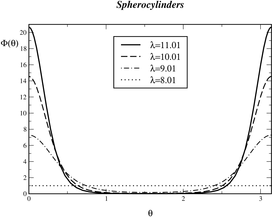
Figure 3: Solutions $\Phi(\theta)=4\pi f(\theta)$ of the Onsager integral equation for spherocylinders for $\lambda^{*}=11.01$, 10.01, 9.01, 8.01.

We have solved the Onsager integral equation for values of $\lambda$ in the range of $\lambda^{*}=2DL^{2}\lambda\in[8:12]$ for spherocylinders, and $\lambda^{*}=2ab^{2}\lambda\in[8:25]$ for ellipsoids, in steps of 0.01. To this end, we have applied an iterative numerical method, which is simple and reliably convergent [48]. The integrals were calculated by the Gauss-Legendre quadrature, using 50 points per integral and checking that with 100 points we get the same results. The initial guess for the highest value of $\lambda^{*}$, $\lambda^{*}=12$ or $\lambda^{*}=25$, was

$$f(\theta,\phi)=\frac{1}{2\pi}\frac{\exp\left(P_{2}(\cos\theta)\right)}{\int du\>\exp\left(P_{2}(u)\right)},$$

where $P_{2}(u)$ is the second Legendre polynomial. At lower $\lambda^{*}$, the iteration was started with the anisotropic solution for the previous, next higher, value of $\lambda^{*}$. The convergence criterion was

$$\left[\sum^{n_{p}}_{i=1}\left[f_{m+1}(\theta_{i})-f_{m}(\theta_{i})\right]^{2}\right]^{\frac{1}{2}}<10^{-6}$$ (29)

where $n_{p}$ refers to the number of points used to perform integrals and m to the mth iteration. The dependence on $\phi$ has been omitted because the distribution function does not actually depend on it. The resulting distribution functions for $\lambda^{*}=11.01$, 10.01, 9.01, 8.01 for spherocylinders are shown in Figure 3. Our orientational distribution functions compare well with those in reference  [49]. Due to the particular shape of the covolume between a pair of spherocylinders, the solutions depend on $\lambda^{*}$, but not on $x$. We found anisotropic solutions for values $\lambda^{*}\geq 8.88$, in agreement with Lasher [50].

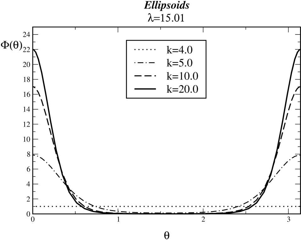
Figure 4: Solutions $\Phi(\theta)=4\pi f(\theta)$ of the Onsager integral equation for ellipsoids for $k=4.0$, 5.0, 10.0, 20.0 at fixed value of $\lambda^{*}=15.01$.

In the case of ellipsoids, the solution for fixed $\lambda^{*}$ depend on the shape anisotropy parameter $k$. In Figure 4, solutions at different value of $k$ are shown for $\lambda^{*}=15.01$. The lowest value of $\lambda^{*}$ which still yields an anisotropic solution is a decreasing function of $k$.

Next we must identify the stable phases and the coexistence line. At coexistence, both the pressure and the chemical potential are equal:

$$P_{N}=P_{i};\qquad\qquad\mu_{N}=\mu_{i}.$$ (30)

We have solved these two equations with Newton’s method, i.e., we found the density $\rho^{P}_{I}$ at which an isotropic phase has the pressure $P_{N}$ and the density $\rho^{\mu}_{I}$ at which an isotropic phase has the chemical potential equal to $\mu_{N}$. At the coexistence line, both densities must be equal. Hence we calculated the nematic $\rho_{N}$ at which $|\rho^{P}_{I}-\rho^{\mu}_{I}|$ was minimal. Usually the value of the minimum was in the range $|\rho^{P}_{I}-\rho^{\mu}_{I}|\in[10^{-9};10^{-5}]$.

The results are shown as a function of the anisotropy in Figure 5 for spherocylinders and in Figure 6 for ellipsoids. They are compared with simulation data of Bolhuis and Frenkel [38], Frenkel and Mulder  [39], and Camp et al. [22].

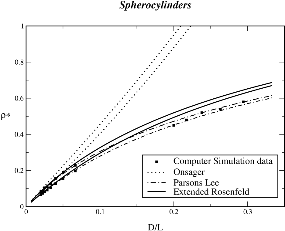
Figure 5: Isotropic-Nematic transition line of hard spherocylinders as a function of elongation $D/L$ and reduced density $\rho^{*}=\rho/\rho_{cp}$ ($\rho_{cp}$ is the density of a close-packed lattice). Solid lines show prediction of our approach (25), dotted line the Onsager result (3), and dashed line the Parsons-Lee prediction (7). Filled squares are simulation results from Bolhuis and Frenkel [38] (for larger $D/L$), only one transition density is given in this reference).

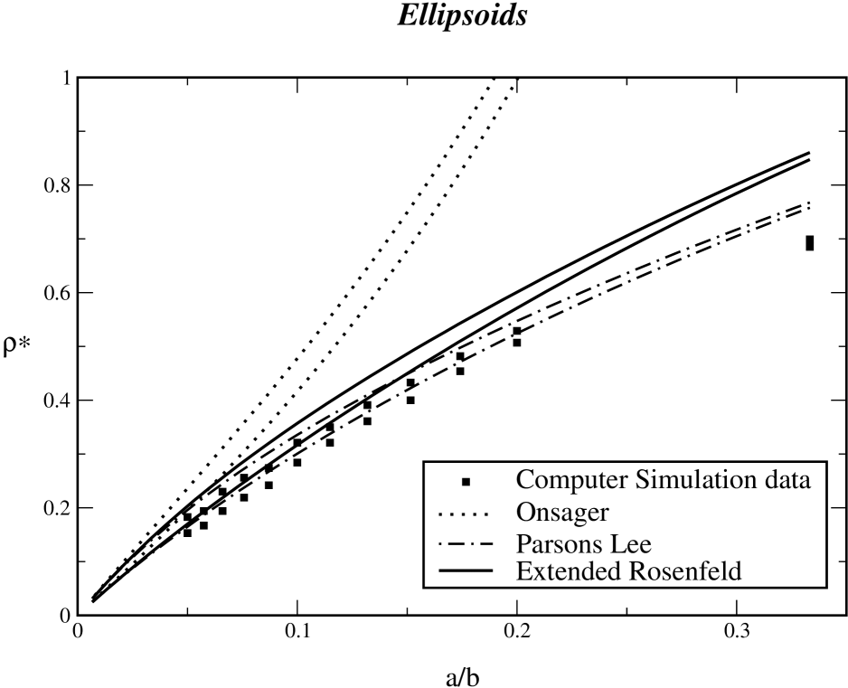
Figure 6: Isotropic-Nematic transition line of hard ellipsoids as a function of elongation $a/b$ and reduced density $\rho^{*}=\rho/\rho_{cp}$ ($\rho_{cp}$ is the density of a close-packed lattice). Solid lines show prediction of our approach (25), dotted line the Onsager result (3), and dashed line the Parsons-Lee prediction (7). Filled squares are simulation results from Camp et al. [22]. The points at $k=3.0$ are taken from Ref.  [39]

The figures demonstrate that our functional performs much better than the Onsager functional, and only slightly worse than the Parsons-Lee functional. As has already been demonstrated elsewhere for spherocylinders and ellipsoids [21, 22], the predictions of the latter are almost exact. The slightly inferior performance of our functional is probably related to the fact that the Parsons-Lee approach is based on the Carnahan-Starling equation of state, whereas the Rosenfeld functional yields the Percus-Yevick equation of state for hard spheres, which is slightly inferior. On principle, one can modify the Rosenfeld functional such that it reproduces the Carnahan-Starling equation of state for fluids, along the lines of an approach suggested by Tarazona [51]. Unfortunately, this is done at the expense of a less accurate description of crystals [51].

Our approach could possibly be improved by making the coefficient of $\Phi_{3}$ in Eqn. (11) dependent on the orientation distribution $f(\varpi)$: formally, the Rosenfeld functional has the form of a third order $Y$-expansion [52]. Mulder and Frenkel  [53] and Tjipto-Margo and Evans [15] have generalized the latter to convex anisotropic bodies and applied it to hard ellipsoids, determining the third virial coefficient numerically. Their nematic-isotropic coexistence densities were lower than those observed in the simulations. In contrast, our functional tends to overestimate the coexistence densities. This suggests that introducing orientation dependent coefficients will shift the transition lines in the correct direction.

However, these modifications complicate the functional. We have shown that already our simple version describes uniform fluids reasonably well. Compared to the Parsons-Lee theory, it has the advantage of being based on a reference density functional which describes the local structure of hard spheres very accurately. It interpolates on the level of the direct correlation function, i. e. the local bulk structure, between the Percus-Yevick solution for hard spheres, which is very good, and the Onsager solution for infinitely elongated particles, which is exact. Therefore, we believe that it will be suited to describe inhomogeneous anisotropic fluids.

5 Summary and Outlook

We have introduced a new density functional for liquid crystals, which interpolates between the successful Rosenfeld functional for hard sphere fluids [2] and the Onsager functional for liquid crystals [12]. As a first test, we have calculated the nematic-isotropic phase diagram for hard spherocylinders and hard ellipsoids and shown that the new functional produces reasonable results. In the next step, it shall be applied to calculate the local liquid structure in homogeneous fluids. For example, direct correlation functions in nematic fluids of ellipsoids have been determined recently from computer simulations [54, 55, 56]. They can also be calculated from our density functional. This will be a second, much more sensitive test of the theory.

If the new functional is successful, it will allow to predict the structure and the properties of nematic liquid crystals in the vicinity of inhomogeneities. It will thus contribute to an improved microscopic understanding of surface phenomena such as surface anchoring on rough and structured surfaces, or of defect structures and defect interactions. It also provides a new approach to smectic ordering, and might lead to useful insight into the nature of the nematic-smectic transition [57].

References

- [1] R. Evans, in Fundamentals of Inhomogeneous Fluids, edited by D. Henderson (Dekker, New York, 1992).
- [2] Y. Rosenfeld, Phys. Rev. Lett. 63, 980 (1989); J. Chem. Phys. 98, 8126 (1993); New Approaches to Problems in Liquid State Theory, p. 303, edited by C. Caccamo et al.(Kluwer Academic, Dordrecht,1999).
- [3] J. P. Hansen and I. R. McDonald, Theory of Simple Liquids (Academic Press, London, 1986).
- [4] Y. Rosenfeld, M. Schmidt, H. Löwen, P. Tarazona, Phys. Rev. E 55, 2425 (1997).
- [5] Y. Rosenfeld, Phys. Rev. Lett. 72, 3831 (1994).
- [6] I. Pagonabarraga, M. E. Cates, G. J. Ackland, Phys. Rev. Lett. 84 911 (2000).
- [7] Y. Rosenfeld, in Chemical Applications of Density-Functional Theory, p. 198, edited by B. Laird, R. Ross, T. Ziegler, ACS Symposium Series Vol. 629 (American Chemical Society, Washington DC, 1996).
- [8] Y. Rosenfeld, Phys. Rev. E 50, R3318 (1994).
- [9] A. Chamoux, A. Perera, J. Chem. Phys. 104, 1493 (1996).
- [10] M. Schmidt, Phys. Rev. E 63, 050201 (2001); M. Schmidt, C. von Feber, Phys. Rev. E 64, 051115 (2001).
- [11] R. Roth, R. van Roij, D. Andrienko, K. R. Mecke, S. Dietrich, Phys. Rev. Lett. 89, 088301 (2002).
- [12] L. Onsager, Ann. N. Y. Acad. Sci. 51, 627 (1949).
- [13] R. Oldenbourg, X. Wen, R. B. Meyer, Phys. Rev. Lett. 61, 1851 (1988).
- [14] Y. Mao, M. E. Cates, H. N. W. Lekkerkerker, J. Chem. Phys. 106, 3721 (1997).
- [15] B. Tjipto-Margo, G.T.Evans, J. Chem. Phys. 93, 4254 (1990).
- [16] J. D. Parsons, Phys. Rev. A 19, 1125 (1979).
- [17] S.-D. Lee, J. Chem. Phys. 87, 4972 (1987); S.-D. Lee, J. Chem. Phys. 89, 7036 (1988).
- [18] A. Samborski, G. T. Evans, C. P. Mason, M. P. Allen, Mol. Phys. 81, 263 (1994).
- [19] P. Padilla, E. Velasco, J. Chem. Phys. 106, 10299 (1997).
- [20] N. F. Carnahan, K. E. Starling, J. Chem. Phys. 51, 635 (1969).
- [21] S. C. McGrother, D. C. Williamson, G. Jackson, J. Chem. Phys. 104, 6755 (1996).
- [22] P. J. Camp, C. P. Mason, M. P. Allen, A. A. Khare, D. A. Kofke, J. Chem. Phys. 105, 2837 (1996).
- [23] M. P. Allen, C. P. Mason, E. de Miguel, J. Stelzer, Phys. Rev. E 52, R25 (1995).
- [24] The direct correlation functions in the Parsons-Lee model are directly proportional to the Mayer-function at all densities.
- [25] N. H. Phuong, unpublished.
- [26] A. Poniewierski, R. Holyst, Phys. Rev. Lett. 61, 2461 (1988); R. Holyst, A. Poniewierski, Phys. Rev. A 39, 2742 (1989); R. Holyst, A. Poniewierski, Mol. Phys. 68, 381 (1990); R. Holyst, A. Poniewierski, Phys. Rev. A 41, 6871 (1990).
- [27] A. M. Somoza, P. Tarazona, Phys. Rev. Lett. 61, 2566 (1988); A. M. Somoza, P. Tarazona, J. Chem. Phys. 91, 517 (1989); A. M. Somoza, P. Tarazona, Phys. Rev. A 41, 965 (1990).
- [28] P. Tarazona, Mol. Phys. 52, 847 (1984); P. Tarazona, R. Evans, Mol. Phys. 52, 847 (1984); P. Tarazona, U. Marini Bettolo Marconi, R. Evans, Mol. Phys. 60, 573 (1987).
- [29] P. Tarazona, Phys. Rev. A 31, 2672 (1985).
- [30] W. A. Curtin, N. W. Ashcroft, Phys. Rev. A 32, 2909 (1985); W. A. Curtin, N. W. Ashcroft, Phys. Rev. Lett. 56, 2775 (1986).
- [31] E. Velasco, L. Mederos, D. E. Sullivan, Phys. Rev. E 62, 3708 (2000).
- [32] H. Graf, H. Löwen, J. Phys. Cond. Matt. 11, 1435 (1999).
- [33] P.Tarazona, Phys. Rev. Lett. 84, 694 (2000).
- [34] Let and be the two local principal curvatures at the surface point . Then the mean curvature is , and the Gaussian curvature, .
- [35] C. E. Weatherburn, Differential Geometry of Three Dimensions (Cambridge University Press, Cambridge, 1961).
- [36] K. Mecke, in preparation.
- [37] Our functional can be cast in the form of a weighted density functional if the weighted densities are allowed to depend on orientations.
- [38] P. Bolhuis, D. Frenkel, J. Chem. Phys. 106, 666 (1996).
- [39] D. Frenkel, B. M. Mulder, Mol. Phys. 55, 1171 (1985).
- [40] A. Isihara, J. Chem. Phys. 19, 1142 (1951).
- [41] J. W. Perram, M. S. Wertheim, J. Comput. Phys. 58, 409 (1985).
- [42] T. Kihara, Rev. Mod. Phys. 25, 831 (1953).
- [43] U. P. Singh, Y. Singh, Phys. Rev. A 33, 2725 (1986).
- [44] J. L. Colot, X. G. Wu, H. Xu, M. Baus, Phys. Rev. A 38, 2022 (1988).
- [45] F. Marko, Phys. Rev. Lett. 60, 325 (1988).
- [46] B. J. Berne, P. Pechukas, J. Chem. Phys. 56, 4213 (1972).
- [47] E. De Miguel, E. Martin del Rio, J. Chem. Phys. 115, 9072 (2001).
- [48] J. Herzfeld, A. E. Berger, J. W. Wingate, Macromolecules 17, 1718 (1984).
- [49] R.Van Roij, B. Mulder, Europhys. Lett. 34, 201 (1996).
- [50] G. Lasher, J. Chem. Phys. 53, 4141 (1970).
- [51] P. Tarazona, Physica A 306, 243 (2002).
- [52] B. Barboy, W. M. Gelbart, J. Chem. Phys. 71, 3053 (1979); B. Barboy, W. M. Gelbart, J. Stat. Phys. 22, 685, 709 (1980).
- [53] B. Mulder, D. Frenkel, Mol. Phys. 55, 1193 (1985).
- [54] N. H. Phuong, G. Germano, F. Schmid, J. Chem. Phys. 115, 7227 (2001); Comp. Phys. Comm., to appear (2002).
- [55] N. H. Phuong, Dissertation, Universität Bielefeld (2002).
- [56] N. H. Phuong, F. Schmid, in preparation.
- [57] Y. Martinez-Raton, J.A. Cuesta, R. van Roij, B. Mulder, in New Approaches to Old and New Problems in Liquid State Theory, p. 139, edited by C. Caccamo et al (Kluwer Academic, Dordrecht, 1999).