Renormalization by Continuous Unitary Transformations: One-Dimensional Spinless Fermions

Abstract

A renormalization scheme for interacting fermionic systems is presented where the renormalization is carried out in terms of the fermionic degrees of freedom. The scheme is based on continuous unitary transformations of the hamiltonian which stays hermitian throughout the renormalization flow, whereby any frequency dependence is avoided. The approach is illustrated in detail for a model of spinless fermions with nearest neighbour repulsion in one dimension. Even though the fermionic degrees of freedom do not provide an easy starting point in one dimension favorable results are obtained which agree well with the exact findings based on Bethe ansatz.

1 Introduction

With the discovery of high temperature superconductivity in layered cuprates of perovskite type bedno86 and the subsequent most intensive theoretical considerations of this intriguing phenomenon (see e.g. Refs. ander97 ; carls02 ) it has become apparent that a reliable approach to strongly interacting fermionic systems is lacking. So the efforts to formulate the very successful concept of renormalization wilso75 also for extended interacting fermionic systems have been intensified considerably during the last decade, see e.g. Ref. shank94 . By now the literature on this approach is so wide that it is not possible to provide an exhaustive list. This underlines the importance that is accorded to this topic.

So far a number of renormalizing schemes has been applied to two-dimensional Hubbard-type models which are relevant for high temperature superconductivity zanch97 ; halbo00a ; honer01a . These schemes rely conceptually on diagrammatic perturbation theory in the interaction strength. They are non-perturbative in the sense that infinite orders of the interaction are kept; the necessary truncation concerns terms of a certain structure, e.g. six points correlations, not terms of a certain order in the interaction. The Fermi surface is discretized and the various scattering couplings across the Fermi sea are suitably parametrized. It is possible to detect whether or not the renormalized couplings decrease of diverge in the course of the flow. In this way, robust evidence for the occurrence of $d$-wave superconductivity was found. The corresponding couplings diverge for certain values of doping and interaction. So far, however, no calculations exist for dynamical correlations like the ARPES response at finite energies and wave vectors (measured relative to the Fermi surface) as required for the understanding of the experimental findings. This is due to the great complexity of the problem which requires – among other difficulties – to follow the flow of the observables as well, see for instance the appendix in Ref. honer01a . For an impurity in a spinless Luttinger liquid a spectral density at all energies was computed by a one-particle irreducible renormalization approach neglecting, however, the renormalization of the two-particle vertex meden02 .

Starting from a flow equation approach as proposed by Wegner wegne94 and quite similarly by Głazeck and Wilson glaze93 ; glaze94 a renormalizing scheme based on continuous unitary transformations (CUTs) has been proposed heidb02a . By an appropriately chosen unitary transformation an effective hamiltonian $H_{\rm eff}$ is obtained. The transformation is tuned in such a way that $H_{\rm eff}$ conserves the number of quasi-particles. Due to this property the calculation of dynamical correlation function for all energies becomes possible as was shown for spin ladders knett01b . For this reason, we consider the renormalizing CUT approach to have a particularly great potential. This expectation is supported decisively by recent work on quantum chemical systems white02 where White could show that the numerical application of a continuous unitary transformation similar to the one used in Ref. heidb02a and here leads to excellent results.

It is the aim of the present work to explain the technical details of the calculations announced in Ref. heidb02a . To this end, intermediate results will be shown. We hope that the available data will make it possible to conceive also analytical treatments which capture the essential physics. The medium-term objective is to generalize the renormalizing CUT approach to more realistic models. A demanding challenge is to treat the dimensional crossover between one- and two-dimensional interacting fermionic models. This is of great experimental relevance since the physical systems existing in nature are at best quasi-one-dimensional, i.e. strongly anisotropic, so that the higher dimensionality enters always at a certain stage.

Two dimensions are the most demanding case for the theoretical description of strong correlations. In three dimensions the powerful Fermi liquid theory is well established which is based on the observation that the quasi-particles as such yield a good description of the low-lying excitations (see e.g. nozie97 ). The interaction between the quasi-particles is not essential. In one dimension on the other hand, the collective plasmon modes dominate the low-energy physics completely so that the fermionic hamiltonian can be mapped to a bosonic one representing so-called Luttinger liquids (see e.g. voit95 ; gogol98 ). This phenomenon can be seen as a binding (or anti-binding) of a pair consisting of a hole and a fermion. This implies that it is a signature of a dominating interaction between the quasi-particles. This fact is commonly interpreted as the failure of a description of the energetically low-lying physics in terms of quasi-particles.

Considering two dimensional strongly interacting systems it is shown that they are generically Fermi liquids in the weak coupling regime feldm95 . So, qualitatively, two dimensional systems are similar to three dimensional ones in the weak coupling limit. But at strong coupling this is no longer true. For given generic hopping element $t$ and interaction strength $U$ the lower dimensional system is more influenced by strong correlations than the corresponding higher dimensional one. This stems from two effects: (i) The band width being proportional to the coordination number is higher in the higher dimensional case. (ii) If collective modes, damped or undamped, are formed their density of states (DOS) at low energies is higher in lower dimensions. For instance, the DOS $\rho(\omega)$ of linear dispersing modes $\omega\propto|{\bf k}|$ behaves like $\rho(\omega)\propto\omega^{d-1}$ with dimension $d$.

In the above sense, two dimensional strongly interacting systems represent an intermediate situation. Generically, neither the interactions between the quasi-particles can be sufficiently described by a Landau function as in three dimensions, nor is the physics completely dominated by collective modes formed from bound particle-hole pairs. Hence, in two dimensions one has to have a theoretical tool which is able to reconcile both main features: collective modes occur and they are important, but they do not exhaust all degrees of freedom. There are also quasi-particles. But their interaction is very important.

The above considerations are the motivation to show here that it is possible to use continuous unitary transformations and quasi-particle description for one dimensional systems to recover the known results. In particular, we will look at the momentum distribution in the ground state which differs significantly between Fermi liquids and Luttinger liquids. In Fermi liquids a jump by $Z_{k_{\rm F}}$, the quasi-particle weight, occurs at the Fermi level whereas in Luttinger liquids only a power-law behaviour occurs voit95 ; gogol98 . Our investigation is intended to be a test case for the method, not as a means to obtain new and so far unknown data. Evidence is provided that in one dimension the physics has not turned bosonic out of the blue but that a description in terms of fermionic quasi-particles is still reasonable even though a description in terms of bosons is easier. In view of the medium-term aim to describe the dimensional crossover we consider the fermionic approach to be a necessary prerequisite.

The paper is set-up as follows. After this Introduction the method is described in Sect. 2. Also the model to which the continuous unitary transformation is applied is given in detail. In Sect. 3 the numerical results are shown and discussed. The comprehensive Discussion concludes the article in Sect. 4.

2 Method and Model

In general, we consider a translationally invariant system of $N$ interacting fermions

$$H = NE+\sum_{k}\varepsilon_{k}:c^{\dagger}_{k}c^{\phantom{\dagger}}_{k}:$$ (1)

$$+\frac{1}{N}\sum_{kqp}\Gamma_{kqp}:c^{\dagger}_{k+q}c^{\dagger}_{k-q}c^{\phantom{\dagger}}_{k-p}c^{\phantom{\dagger}}_{k+p}:\ .$$

Here $c^{\dagger}_{k}$ ($c^{\phantom{\dagger}}_{k}$) creates (annihilates) a fermion at wave vector $k$ in momentum space. Note that the parametrization of the scattering processes is not the conventional one. Our choice, however, is more apt to represent the inherent symmetries (see below). The fermions appearing are considered to be spinless, i.e. there is at maximum one per site and no spin index occurs. The colons $:\ldots:$ denote normal ordering with respect to the non-interacting Fermi sea. This commonly used classification makes it easier to trace the effect of the individual terms (cf. appendix A). The function $\Gamma_{kqp}$ is the vertex function embodying the amplitudes for all possible scattering processes.

2.1 Method

The method which we use to analyse the hamiltonian (1), is the method of continuous unitary transformations (CUTs) based on the flow equation approach proposed by Wegner wegne94 . The unitary transformation $U(\ell)$ is parametrized by the continuous variable $\ell$ ranging between $0$ and $\infty$. A given hamiltonian $H(0)$ is continuously mapped onto an effective model $H_{\rm eff}$ as $\ell$ is taken from zero to infinity. The continuous unitary transformation is defined locally in $\ell$ by the antihermitian generator $\eta(\ell)$

$$\frac{d}{dl}H(\ell)=\left[\eta(\ell),H(\ell)\right]\ .$$ (2)

Of course, all other observables $O$ have to be subject to the same transformations

$$\frac{d}{dl}O(\ell)=\left[\eta(\ell),O(\ell)\right]$$ (3)

since the expectation values and correlations shall not be altered by the transformation.

The main task is to determine $\eta(\ell)=\eta(H(\ell))$ in a way that brings the hamiltonian systematically closer to a simpler structure. Once the generator is chosen and the commutator calculated, one obtains a high dimensional set of coupled ordinary differential equations. These have to be solved in the limit $\ell\to\infty$.

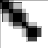
$\Longrightarrow$

Figure 1: Hamiltonian with a block band structure transformed into an effective block diagonal hamiltonian. Each black block stands for the action of the hamiltonian in a subspace of the Hilbert space with a given number of excitations. Let us assume that the uppermost block stands for the vacuum (no excitation); the next lower block acts on states with one single excitation; the next lower block acts on states with two excitations and so on. In the example depicted the number of excitations can change at most by two on a single application of the hamiltonian. This is the block band structure.

For the choice of $\eta(\ell)$ we focus on the case where the original hamiltonian $H$ has a so called block band structure with respect to a certain counting operator $Q$, i.e. an operator with a spectrum of non-negative integers. The operator $Q$ shall be the operator counting the number of excitations present in the system. The ground state $|0\rangle$ of $Q$, the so-called quasi-particle vacuum, is the state without any excitation so that

$$Q|0\rangle=0$$ (4)

holds. The block band structure occurs if the whole hamiltonian $H$ changes the counting operator $Q$ at maximum by a certain value $M<\infty$. This means that $H$ links two eigen states $|i\rangle$ and $|j\rangle$ of $Q$ only if their eigen values $q_{i}$ and $q_{j}$ differ at most by $M$: $|q_{i}-q_{j}|\leq M$. In Fig. 1 the case $M=2$ is illustrated.

In view of systems of interacting fermions (1) we choose $Q$ to be the operator counting the number of quasi-particles, i.e. the number of particles above the Fermi level plus the number of holes below

$$Q=\sum_{k}\mbox{sign}(|k|-k_{\rm F}):c^{\dagger}_{k}c^{\phantom{\dagger}}_{k}:\ .$$ (5)

This choice implies that we intend to use ordinary quasi-particles as the elementary excitations. Generally, we like to stress that the choice of $Q$ requires some physical intuition or a certain presumption about the problem under study. The choice of $Q$ can be considered as the choice of a starting point. Depending on the quality of this choice subsequent approximations will be more or less reliable. This point will be discussed below in more detail.

First, however, we turn to the choice of the generator. For band-diagonal matrices Mielke proposed an ansatz mielk98 that was generalized to many-body problems with block-band structures by Knetter and Uhrig knett00a . The antihermitian generator $\eta(\ell)$ is chosen such that its matrix elements are given in an eigen basis of $Q$ by

$$\eta_{ij}(\ell)=\mbox{sign}(q_{i}(\ell)-q_{j}(\ell))H_{ij}(\ell)\ .$$ (6)

For the interacting fermions as in (1) the conventional occupation number basis is appropriate.

Since in general the eigen space for a given number of excitations $q_{i}$ has a finite dimension we use the convention that $A_{ij}$ is not only a single matrix element but the whole submatrix of $A$ which connects the eigen space belonging to $q_{j}$ (domain) to the eigen space belonging to $q_{i}$ (co-domain). With this convention Eq. 6 becomes a matrix equation. Inserting Eq. 6 into the general flow equation (2) yields

$$\frac{d}{dl}H_{ij}=-\mbox{sign}(q_{i}-q_{j})(H_{ii}H_{ij}-H_{ij}H_{jj})$$

$$\quad+\sum_{k\neq ij}\left(\mbox{sign}(q_{i}-q_{k})+\mbox{sign}(q_{j}-q_{k})\right)H_{ik}H_{kj}$$ (7)

which is also a matrix equation, i.e. the sequence of the matrices in the products matters. One can show mielk98 ; knett00a that (7)

• preserves the block band structure and

• leads to a block diagonal $H_{\rm eff}$ where $q_{i}\neq q_{j}\Rightarrow H_{{\rm eff},ij}=0$. The condition necessary for these conclusions is that the spectrum of the hamiltonian is bounded from below which constitutes a natural assumption for physical systems.

The block diagonality of the effective model is equivalent to the commutation of the effective model with $Q$ $[Q,H_{{\rm eff}}]=0$.

Furthermore, we show that the ground state of the system is mapped onto the state with no elementary excitations, i.e. the vacuum $|0\rangle$ without any excited quasi-particles, in the course of the transformation. Let us assume that the ground state is not degenerate. Without loss of generality the indexing is chosen such that $i=0$ refers to the vacuum with $q_{0}=0$. For $j=0$ we obtain from (7)

$$\frac{d}{dl}H_{i0} = -(H_{ii}H_{i0}-H_{i0}E)$$ (8)

$$+\sum_{k\neq i0}\left(\mbox{sign}(q_{i}-q_{k})-1)\right)H_{ik}H_{k0}\ ,$$

where $E:=\langle 0|H|0\rangle=H_{00}$ is the energy of the vacuum. $H_{i0}$ is a vector that connects the vacuum with other states. For large $\ell$ the flow has led the system already close to block diagonality mielk98 ; knett00a . Then the matrices $H_{ik}$ linking blocks of different number of elementary excitations are small quantities so that Eq. (8) is dominated by the first term on the right hand side. The products $H_{ik}H_{k0}$ in the sum are smaller by one order in the off-diagonal matrices. So the asymptotic behaviour is given by

$$\frac{d}{dl}H_{i0}\approx(E-H_{ii})H_{i0}\ .$$ (9)

Since $H_{i0}$ has to tend to zero due to the general convergence mielk98 ; knett00a we deduce from (9) that $E-H_{ii}\leq 0$ for large $\ell$. This implies that $E$ is lower in energy than any state different from the vacuum which is linked to the vacuum by a non-zero element $H_{i0}$. We interprete the physical content of this result in the following way. In a block band diagonal hamiltonian as illustrated on the left side in Fig. 1 the vacuum is linked to states with a certain finite number (bounded by $M$) of elementary excitations. From (9) we learn that the vacuum is lower in energy than those states. Generically, this implies that also all other states which contain an unrestricted number of elementary excitations lie higher in energy. We conclude that the vacuum is indeed the ground state unless a phase transition takes place.

To illustrate the latter statement in more detail let us think about a hamiltonian which is controlled by an interaction parameter $U$ such that the vacuum is the ground state for $U=0$ without any transformation. Then the situation changes gradually and smoothly as $U$ is turned on so that the ground state is mapped onto the vacuum. This is true till a singularity occurs, that is a phase transition. A second order phase transition would be signaled by the softening – vanishing of the eigen energy – of one of the excited states (for an example see the single triplet excitation in Ref. knett00b ). Technically, this implies that the convergence of $H_{i0}$ as given by Eq. (9) breaks down since the expression in the bracket on the right hand side vanishes. This reflects the physical fact that our approach will not work beyond the phase transition since there the original vacuum is no longer a good reference state for the true ground state. But it is possible to use the approach until the phase transition is reached and the second order phase transition can be detected by the vanishing of the energy of one of the excited states.

First order transitions spoil also the applicability of a smooth mapping. But they cannot be detected locally. A first order jump occurs when a completely different state comes down in energy. Such a completely different state is built from a macroscopic number of elementary excitations and will in general not be connected to the vacuum by a finite element $H_{i0}$. This means that the smooth mapping constructed by the CUT may still work even though a first order transition has occurred simply because there is no local connection of the local energy minimum, which is mapped to the vacuum, to the global one. This concludes the general considerations about the mapping generated by the CUT between the ground state and the vacuum of elementary excitations.

Now we return to the model of interacting fermions in (1). Inspection shows that this model has a block band structure with respect to the counting operator (5) of quasi-particles. If a particle from below the Fermi level is scattered to a state above the Fermi level two elementary excitations are created: one hole and one particle. The inverse process corresponds to the decrement of the number of quasi-particles by two. If the particle is scattered from below the Fermi level to below the Fermi level the number of quasi-particles remains constant. The same is true if the particle is taken from above the Fermi level to another state above this level. If we consider at maximum scattering terms built from four fermionic operators, as it is done in Eq. (1), then two fermions are scattered so that the possible changes in the number of quasi-particles are $0,\pm 2,\pm 4$. So there is a natural upper bound $M=4$ and the system displays indeed a block band structure. Note that all the statements so far were independent of the dimension of the model.

2.2 Model

The explicit model we consider here is a system of one-dimensional spinless fermions. Haldane used it to explain the concept of Luttinger liquids halda81b . Physical realizations one may think of are either completely polarized electrons or anisotropic spin chains which can be rigorously mapped onto spinless fermions by means of the Jordan-Wigner transformation fradk91 . A completely different application is the description of vicinal surfaces where the hard-core repulsion between different steps is taken into account by passing to fermions joos91 .

The model is a tight-binding model where the particles are distributed over a one-dimensional chain of $N$ sites with antiperiodic boundary conditions at half filling, i.e. on average each site is occupied by half a fermion. The fermions can hop to nearest neighbour sites and there is a repulsive interaction $V$ between two adjacent fermions

$$H=\sum^{N}_{i=1}\left[{\textstyle\frac{1}{2}}(a^{\dagger}_{i+1}a^{\phantom{\dagger}}_{i}+\mbox{h.c.})+V\left(n_{i+1}-{\textstyle\frac{1}{2}}\right)\left(n_{i}-{\textstyle\frac{1}{2}}\right)\right]\,,$$ (10)

where $a^{\dagger}_{i}$ ($a^{\phantom{\dagger}}_{i}$) creates (annihilates) a fermion on site $i$ in real space. This model is exactly solvable in the form of an anisotropic spin model. The solution is due to Bethe bethe31 and to Yang and Yang yang66a ; yang66b . More results were found later johns73 ; luthe75 ; halda80 ; halda81a ; halda81b . In the present context it is important to know that the system is metallic for not too large couplings, namely for $V\leq 1$. In this region it is the simplest realistic tight-binding model displaying Luttinger liquid behaviour which is why we use it as our test case. At the value $V=1$ a continuous phase transition takes place into a charge density wave where the fermion density is staggered. Thus the translation symmetry of the system is spontaneously broken. This phase displays also a charge gap and represents hence an insulator. In the present work, however, our interest is focused on the metallic phase.

Representation

Let us first clarify the notation that we use in the following. Transforming the real-space representation (10) into momentum-space and normal-ordering of the hamiltonian with respect to the non-interacting Fermi sea yields a hamiltonian of the form in Eq. (1) with the coefficients

$$E = -\left({\textstyle\frac{1}{\pi}+\frac{V}{2\pi}}\right)$$ (11)

$$\varepsilon_{k} = -\left(1+{\textstyle\frac{2V}{\pi}}\right)\cos k$$ (12)

$$\Gamma_{kqp} = {\phantom{-}}V\sin q\sin p\ .$$ (13)

in the thermodynamic limit $N\to\infty$. For finite system sizes $N<\infty$ as used below the dispersion reads

$$\varepsilon_{k}=-\left(1+{\frac{2V}{N}}\sum_{|k^{\prime}|<k_{\rm F}}\cos k^{\prime}\right)\cos k\ .$$ (14)

The terms $\frac{1}{\pi}$ and $\frac{V}{2\pi}$ in $E$ correspond to the ground state energy of the non-interacting system and to the Fock term, respectively. We are not interested in these leading order effects but will concentrate on the correlation effects as they appear in the subsequent orders.

Based on the parametrization chosen in Eq. (1) the symmetries and notation properties of the system manifest themselves in a very concise way in the vertex function $\Gamma_{kqp}$

1. hermitecity leads to

   $$\Gamma_{kqp}=\Gamma_{kpq}\ ,$$ (15)

2. inversion symmetry leads to

   $$\Gamma_{kqp}=\Gamma_{-k-q-p}$$ (16)

3. particle-hole symmetry leads to

   $$\Gamma_{kqp}=\Gamma_{k+\pi qp}=\Gamma_{kq+\pi p+\pi}\ .$$ (17)

A swap of two neighboured fermionic operators in a normal-ordered product leads only to an additional minus sign. Thus there is a redundancy in the notation $:c_{1}c_{2}\ldots:=-:c_{2}c_{1}\ldots:$ which implies that $\Gamma_{kqp}$ is not uniquely defined by Eq. (1). This caveat can be remedied by the additional requirement of the

1. notation symmetry

   $$\Gamma_{kqp}=-\Gamma_{k-qp}=-\Gamma_{kq-p}\ .$$ (18)

The notation symmetry implies that the momentum dependence of the vertex function is the one given in (13). Note that in our notation the vertex function $\Gamma_{kqp}$ vanishes automatically if fermions are scattered from the Fermi points to the Fermi points ($k=\pm\pi/2$ and $q,p\in\{0,\pm\pi\}$). This important fact leads to the property that the interaction is not a relevant perturbation but only a marginal one. The CDW does not occur at arbitrarily small interaction but only beyond a finite threshold. If the scattering is denoted in the usual way a much more elaborate reasoning computing the contribution of the Cooper pair and the zero sound channel is required to yield the same result shank91 ; shank01 .

Exploiting the above symmetries the number of non-zero scattering amplitudes that has to be dealt with is reduced from $N^{3}$ to approximately $\frac{N^{3}}{32}$.

Exact Results

Here we report some exact results to which we will compare our findings.

1. The ground state energy per site in the metallic phase $V<1$ reads yang66a

   $$\frac{E}{N}(V)=\frac{\cos\mu}{4}-\sin^{2}\mu\!\!\!\int\limits^{\infty}_{-\infty}\!\!\!\frac{dx}{2\cosh\pi x(\cosh 2x\mu-\cos\mu)}\ ,$$ (19)

   where $V=\cos\mu$. Eq.(19) is dominated by its linear part $-(\frac{1}{\pi}+\frac{V}{2\pi})$ (cf. Eq. (11)), which we will substract to focus on the correlation part of the energy.

2. We deduce from the dispersion of the anisotropic Heisenberg model johns73 the dispersion of the effective fermionic model

   $$\varepsilon_{k}=-\underbrace{\left(\frac{\pi}{2\mu}\right)}_{v^{*}_{\rm F}(V)}\cos k\ ,$$ (20)

   which we expect after the CUT. In particular, we use the value of the Fermi velocity $v^{*}_{\rm F}$ as done previously halda81a . This quantity is also dominated by a rather trivial linear term $1+\frac{2V}{\pi}$ (cf. Eqs. (12,14)) which we will subtract in order to focus on the correlation effects.

3. The momentum distribution $n(k)$ in the ground state cannot be computed directly with Bethe ansatz. But it is possible to deduce the asymptotic behaviour for momenta close to the Fermi wave vector $k_{\rm F}$ based on the representation of the model in terms of bosonic degrees of freedom halda81a . In the momentum distribution a characteristic signature of Luttinger liquid behaviour shows up. No finite jump in $n(k)$ exists at $k=\pm k_{\rm F}$ but a power law singularity with non-universal exponent appears. This singularity is of the form halda81a (for more details, see e.g. meden92 ; voit95 )

   $$n(k\approx k_{\rm F})\approx{\textstyle\frac{1}{2}}-C_{1}\mbox{sign}(k-k_{\rm F})|k-k_{\rm F}|^{\alpha}$$ (21)

   with

   $$\alpha(V) = \frac{1}{\eta(V)}+\frac{\eta(V)}{4}-1$$ (22)

   $$\eta(V) = \frac{\pi}{\pi-\arccos V}$$ (23)

   and an undetermined constant $C_{1}$.

2.3 The Continuous Unitary Transformation

In the subsection on the method 2.1 it was explained that the block band structure of the system is preserved under the chosen CUT. This means that the number of quasi-particles is altered at maximum by $4$. It must be emphasized, however, that this does not imply that only terms made from four fermionic operators, so-called 2-particle operators, occur in the hamiltonian. Even though the initial hamiltonian (1) contains only 0-particle (constants), 1-particle (of the form $:c^{\dagger}c:$) and 2-particle terms (of the form $:c^{\dagger}c^{\dagger}cc:$) the transformation may and will generate also 3-(and more) particle terms. But these terms have to fulfill the condition that they change the number of quasi-particles by no more than $\pm 4$.

Let $T^{(j)}_{i}(\ell)$ be the normal-ordered $j$-particle term in $H(\ell)$ which changes the number of quasi-particles by $i$. So the general structure during the transformation is

$$H(\ell) = T^{(0)}_{0}(\ell)+T^{(1)}_{0}(\ell)+$$ (24)

$$\sum_{j\geq 2}\left[T^{(j)}_{+4}+T^{(j)}_{+2}+T^{(j)}_{0}+T^{(j)}_{-2}+T^{(j)}_{-4}\right]\!(\ell)$$

and

$$\eta(\ell)=\sum_{j\geq 2}\mbox{sign}(i)T^{(j)}_{i}(\ell)\ .$$ (25)

Note that the 1-particle term cannot change the number of quasi-particles since the conservation of momentum does not allow to shift the particle in momentum-space.

Some general analysis is possible. One can study which combinations of $T^{(j^{\prime})}_{i^{\prime}}$ and $T^{(j^{\prime\prime})}_{i^{\prime\prime}}$ in $[\eta(\ell),H(\ell)]$ influence $\frac{d}{dl}T^{(j)}_{i}$. First, the changes in the number of quasi-particles is additive $i=i^{\prime}+i^{\prime\prime}$. Second, the maximum value of $j$ is

$$j_{\rm max}=j^{\prime}+j^{\prime\prime}-1$$ (26)

due to the properties of the commutator between products of fermionic operators. Third, the normal ordering yields also a lower bound for $j$ because the number of possible contractions is restricted. Contractions in a product made from normal-ordered factors are possible only between the fermionic operators from different normal-ordered factors, see Appendix A. So we are led to heidb01

$$j_{\rm min}=$$ (27)

$$\frac{1}{2}\mbox{max}\left\{{{(j^{\prime}+i^{\prime})+(j^{\prime\prime}-i^{\prime\prime})+|(j^{\prime}-i^{\prime})-(j^{\prime\prime}+i^{\prime\prime})|}\atop{(j^{\prime}-i^{\prime})+(j^{\prime\prime}+i^{\prime\prime})+|(j^{\prime}+i^{\prime})-(j^{\prime\prime}-i^{\prime\prime})|}}\right\}\,.$$

It is also possible to derive a set of abstract differential equations for the coefficients of all possible terms. But its structure is quite complicated heidb01 . So a solution of the complete CUTs seems to be hardly accessible and we refrain from persuing this route further and turn to a numerical treatment of finite-size systems with $N$ sites. Still further approximations are necessary because the number of different $j$-particle processes grows generically as $N^{j-1}$.

2.4 Self-Similar or Renormalizing Approximation

We analyse the flow of all terms of the form

$$T^{(0)}_{0}(\ell) = E(\ell)$$ (28)

$$T^{(1)}_{0}(\ell) = \sum_{k\in[0,2\pi)}\varepsilon_{k}(\ell):c^{\dagger}_{k}c^{\phantom{\dagger}}_{k}:$$ (29)

$$T^{(2)}_{i}(\ell) = \sum_{{{k\in[0,\pi)}\atop{qp\in[0,2\pi)}}}\Gamma_{kqp}(\ell):c^{\dagger}_{k+q}c^{\dagger}_{k-q}c^{\phantom{\dagger}}_{k-p}c^{\phantom{\dagger}}_{k+p}:$$ (30)

with $i\in\{0,\pm 2,\pm 4\}$. Terms involving interactions dealing with more than two particles $T^{(j>2)}_{i}$ are neglected. So we proceed as follows. The sum (24) of the terms in Eqs. (28,29,30) represents the hamiltonian at a given value of $\ell$. The corresponding generator $\eta$ in Eq. (25) contains the same terms. This ansatz is inserted at the right hand side of the general flow equation (2). The commutator is computed and the result is normal-ordered (cf. appendix A). The 3-particle terms are omitted and the coefficients of the 0-, 1- and 2-particle terms are compared. In this way, a high dimensional set of ordinary differential equations for the coefficients of the terms in Eqs. (28,29,30) is obtained. These equations are given in appendix B. At $\ell=\infty$ the parts of the third term (30) which alter the number of quasi-particles will have vanished so that only the $i=0$ part remains (for illustration see Fig. 3). At this stage, i.e. at the end of the transformation, $T^{(0)}_{0}$ is the ground state energy, $T^{(1)}_{0}$ the 1-particle dispersion and $T^{(2)}_{0}$ represents the interaction of two quasi-particles. The latter does not need to be small.

Since the given structure of the initial hamiltonian $H(\ell=0)$ is preserved we call this approximation “self-similar” in the spirit of the work by Głazeck and Wilson glaze93 . The naming “renormalizing” is based on three facts. First, on the technical level the coefficients appearing in the initial hamiltonian are changed, i.e. renormalized, in the course of the transformation. Second, the procedure is non-perturbative since terms are omitted not because they are of a certain order in the initial interaction $V$ but because of their structure being 3-(or more) particle terms. This implies that the couplings kept acquire infinite orders in $V$. Third, the generator (6,25) which we use here leads to a smooth exponential cutoff $\exp(-|\Delta E|\ell)$ of the matrix elements connecting states of different energy (energy difference $\Delta E$) mielk98 ; knett00a . Thus matrix elements between energetically distant states are suppressed much more rapidly than those which are energetically very close to each other. This is similar to what is done in Wilson’s renormalization wilso75 where the degrees of freedom at large energies are integrated out first.

We illustrate the exponential cutoff for matrix elements connecting to the ground state. Their asymptotic behaviour on $\ell\to\infty$ is governed by Eq. (9). Let us assume that the non-diagonal elements $H_{i0}$ are already very small. Then the diagonal energies like $E$ and $H_{ii}$ deviate from their asymptotic values only quadratically in the non-diagonal elements as results from second order perturbation theory. So in leading order the diagonal elements can be considered constant in $\ell$. Then Eq. (9) yields $H_{i0}\propto\exp(-(H_{ii}-E)\ell)$ as stated before.

How can the restriction to the terms in Eqs. (28,29,30) be justified? One argument results from considering an expansion in the interaction $V$. The 3-particle interactions neglected are generated by a commutator of two normal-ordered 2-particle terms which are of the order of $V$ so that they are of the order $V^{2}$. For our purposes it is important to know in which order the terms kept are influenced by the neglect of the 3-particle terms. The 3-particle terms can have an influence on the terms kept only if they are commuted again with at least a 2-particle term of the order $V$ or higher. Hence the neglect of the 3-particle terms introduces deviations only in order $V^{3}$. This holds for the 1- and 2-particle terms (29,30). The 0-particle term, which becomes at $\ell=\infty$ the ground state energy, is not changed by the commutator of a 2-particle and a 3-particle term since the generated terms cannot be contracted completely as stated by Eq. (27). So the deviation in the 0-particle term engendered by the neglect of the 3-particle terms is at worst of order $V^{4}$. Thus the approximation can be justified for low values of $V$.

Another argument, which is more general than a power counting in the interaction, comes from the structure of the terms neglected. Let us focus on the 3-particle terms. Since they may change the number of quasi-particles at most by $4$ they contain at least one annihilator of a quasi-particle. Since they are normal-ordered this annihilator appears rightmost. Hence such a term is active only if applied to a state which contains already some excitations. Hence the approximation chosen is justified if the system can be considered a dilute gas of quasi-particles irrespective of the strength of the interaction between the quasi-particles. In the course of the transformation virtual processes creating and annihilating quasi-particles are more and more suppressed so that the average concentration of quasi-particles decreases gradually. Hence towards the end of the transformation the neglect of 3-(and more) particle terms is well justified. On the other hand, the 3-(and more) particle terms are not present in the initial hamiltonian (1) so that their neglect is well justified during the first phase of the transformation as well. Only during the intermediate phase there is no general control of the quality of the approximation. Here one has to focus on the particular system under study. To assess the quality of the approximation one may either compare to otherwise available data on the system (external quality control) or one may compute some of the terms neglect in order estimate how large they are (internal or self-consistent quality control). In the present work we will use the first method and assess the quality of our findings by comparing them to the known exact results. Summarizing, the approximation is well justified if the system can be considered a dilute gas of quasi-particles independent of the actual interaction between the quasi-particles.

Finally, we wish to point out an analogy between our approach and a more standard diagrammatic one. By restricting ourselves to the terms in Eqs. (28,29,30) we are dealing with a 2-particle irreducible vertex function which is renormalized continuously. The renormalization equation (see appendix B) is bilinear in all coefficients. The terms contributing to $\partial_{\ell}\Gamma$, which are bilinear in the vertex function $\Gamma$, result from the commutation and a single contraction of two 2-particle irreducible vertex functions. In this sense our procedure bears similarities to a 1-loop renormalization or to the summation of all parquet diagrams solyo79 . The main difference is that our approach keeps the problem local in time along the renormalization flow because the transformation is unitary. Hence not frequency dependence enters. We consider this a major advantage of the CUT approach for numerical application since much less bookkeeping is required since no frequency dependence has to be traced.

3 Numerical Results

We turn now to the numerical solution of the differential equations set up in appendix B. The momentum dependence of all functions is discretized in an equidistant mesh. The positions of the points of this mesh are chosen such that no $k$-point lies precisely at $k=\pm k_{\rm F}=\pm\pi/2$. For $N$ divisible by 4, this corresponds to antiperiodic boundary conditions. In this way unnecessary degeneracies are avoided. For large system size the influence of the boundary conditions becomes increasingly unimportant.

For the system sizes ($N\approx 50$) that we will be looking at there are about 50.000 coupling constants which are traced in the set of differential equation. Luckily, the differential equations are not very sensitive since they describe the convergence to a static fix point. The numerics is done by a Runge-Kutta algorithm with adaptive stepsize control. This algorithm is robust but quite laborious because the differential equations have to be evaluated six times for each step. Rigorously, the fix point is reached at $\ell=\infty$. In practise, we stop the flow when the relative change of $E$ and $\varepsilon_{k}$ falls below $10^{-6}$.

3.1 Illustration of the CUTs

         

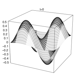
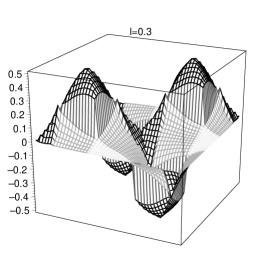
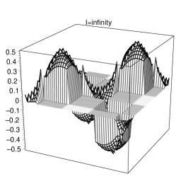
Figure 2: Sections of the vertex function $\Gamma_{kqp}$ at $k=\frac{\pi}{4}$ as function of $q,p\in\{-\pi,\pi\}$ at three values of $\ell$ ($0,0.3$ and $\infty$) for $V=0.5$ and $N=48$ sites. The lightest parts are those that change the number of quasi-particles by $\pm 4$, the gray parts change them by $\pm 2$, the black parts leave it unchanged. The quasi-particle-number changing amplitudes are transformed to zero.

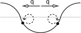
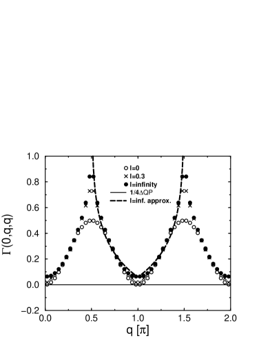
(a) Symmetric replacement

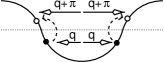
(b) Symmetric scattering of two particles creating (annihilating) four quasi-particles

Figure 3: Sections of the vertex-function $\Gamma_{kqp}$ as in $\Gamma_{kqp}:c^{\dagger}_{k+q}c^{\dagger}_{k-q}c^{\phantom{\dagger}}_{k-p}c^{\phantom{\dagger}}_{k+p}:$. The pictograms illustrate the scattering processes. They show the dispersion (solid line), filled dots for the fermions to be annihilated and open dots for the holes the fermions are put. The arrows depict how the processes change on varying the momentum. $\Delta$QP denotes the change of the number of quasi-particles induced by the scattering process. Note that $\Delta$QP $\neq 0$ implies that the amplitude vanishes for $\ell=\infty$.

         

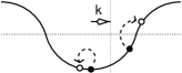
(c) Changing the average momentum $k$ keeping one scattering process unchanged

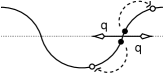
(d) From forward-scattering ($q\approx 0$) to umklapp-scattering ($q\approx\pi$) and back ($q\approx 2\pi$)

Fig. 3 illustrates what the continuous unitary transformations are doing. The parts of the vertex-function that are associated with processes that change the number of quasi-particles are transformed away as $\ell$ goes to $\infty$ while the other part is renormalized. At the end of the transformation there are discontinuities at the borderlines of the different parts and some singular kinks if the scattering processes occur at the Fermi points or if $p=q$ holds.

A more quantitative insight is given by Fig. 3(b) where one-dimensional sections of the vertex-function $\Gamma_{kqp}$ are shown.

• Fig. 3(a) depicts $\Gamma_{0qq}$ for various values of $\ell$. These amplitudes are related to processes where two fermions at $q$ and $-q$ are first annihilated and then created again. The shape of the function close to $|q|=\pi/2$ can be fitted by $\Gamma_{0qq}\approx-0.007q^{2}-0.266\ln||q|/\pi-0.5|-0.125$. So a logarithmic singularity at $\frac{\pi}{2}$ can be presumed.

• In Fig. 3(b) the amplitudes of processes are shown where two fermions are taken from $q$ and $-q$ and put at $\pi-q$ and $-\pi-q$. All these processes change the quasi-particle number and, hence, have to vanish for $\ell\to\infty$. The processes near the Fermi wave vector $q\approx\frac{\pi}{2}$ are decreasing very slowly.

• For the plots in Fig. 3(c) we fix one shift of a fermion from below the Fermi level to an energy above it. The shift of the other fermion is varied. Here, different changes in the number of quasi-particles are possible. There are regions where the amplitudes vanish and others where they are only renormalized. The process at $k=\frac{\pi}{2}$ is apparently different. It corresponds to the exchange of the two particles. At present, we cannot judge whether this difference will be relevant in the thermodynamic limit. It is an interesting question whether it retains a finite weight for $N\to\infty$.

• In Fig. 3(d) we show the evolution of a scattering event from pure exchange at $q=0$ at the right Fermi point over forward-scattering for small positive values of $q$ to umklapp-scattering at $q=\pi$. One realizes that the scattering amplitudes at $q=0$ and at $q=\pi$ are particularly enhanced by the renormalization. It seems totally inappropriate to approximate the scattering amplitudes as being constant for small momentum ($q\approx 0$) or for large momentum ($q\approx\pi$) because the points $q=0$ and $q=\pi$ appear to be decisively different from the scattering in their vicinity. This observation makes the question whether a continuum description is quantitatively applicable an interesting issue for future studies.

3.2 Convergence

Figure 4: Interaction values above which the approximation breaks down because of loss of convergence. Filled symbols stand for numerically stable runs, open symbols ($N\geq 52$) for runs where numerical inaccuracies spoil the convergence. The dashed line extrapolates the numerically reliable results (see Eq. 31).

General statements on the convergence of the CUT approach chosen are possible mielk98 ; knett00a . But they do not ensure that the method works for macroscopically large systems. Additionally, the unavoidable use of approximations may lead to the break down of convergence. So we investigated empirically up to which value of the interaction $V_{\rm crit}$ the CUT works. This value depends on the system size $N$ or the density of the discretization mesh, respectively. If $V$ is larger than $V_{{\rm crit.}}(N)$ all couplings are diverging at a certain $\ell$ and the solution of the differential equations cannot be continued asymptotically to $\infty$. Furthermore, $V_{{\rm crit.}}(N)$ is decreasing as $N$ is growing. In addition, numerical problems occur at system sizes $N>52$ and $V$ close to $V_{{\rm crit.}}(N)$ due to accumulated inaccuracies. This can be seen in the unsystematical behaviour of $V_{{\rm crit.}}(N)$ above $N=52$ and in the unphysical shape of e.g. the dispersion for $V$ close to $V_{{\rm crit.}}(N)$ in Fig. 7. On the other hand, the decrease of $V_{{\rm crit.}}(N)$ is very systematic as long as $N\leq 52$ holds. It can be approximated very well by a linear dependence

$$V_{{\rm crit.}}(N)\approx{9.06/N}+0.75\ ,$$ (31)

which leads to an extrapolated value in the thermodynamic limit $N\to\infty$ of $V_{{\rm crit.}}(\infty)\approx 0.75$. We conclude that it is possible to study the metallic phase of the system and that the conclusions drawn from the finite-size calculations are also relevant for the thermodynamic limit. A description of the transition to the insultating phase is presently not possible.

The Case $N=4$

Some insight on the cause for the loss of convergence can be obtained in the simple case of four points in momentum space, which is analytically solvable with and without approximation. The analytic solution is simple because the quasi-particle vacuum $|\psi_{0}\rangle$ is connected by the interaction only to the state where both fermions are excited $|\psi_{\scriptsize ex.}\rangle$. Thus one has to diagonalize a $2\times 2$ matrix which can be done easily directly or using the CUT.

Our approximation, however, is dealing with operators and not with matrix elements. The state $|\psi_{\scriptsize ex.}\rangle$ involves four quasi-particles - two holes and two excited particles. In the approximation 3- and 4-particle terms are neglected so that the energy of the excited state is incorrect. Indeed, the gap between the ground state and the excited state is under-estimated. It even closes for $V\geq\sqrt{8}$ and the couplings diverge before reaching $\ell=\infty$. Thereby, it is shown that the approximation may spoil the applicability of the approach.

3.3 Ground State Energy per Site

Figure 5: CUT results for the correlation part, i.e. beyond linear order, of the ground state energy per site for various system sizes $N$.

Figure 6: Comparison of the CUT results ($N=48$) for the correlation part of the ground state energy per site with the exact thermodynamic result.

In Fig. 5 we plot the shape of the non-linear lowering of the ground state energy, i.e. the correlation part of the ground state energy, for various system sizes $N$ as obtained by CUT. The ground state energy diverges to negative values close to $V_{{\rm crit.}}(N)$. For $V$ smaller than the extrapolated value $V_{{\rm crit.}}(\infty)$ all systems show nearly the same dependence on the interaction $V$.

The case $N=48$ is compared to the exactly known thermodynamic result yang66a ; yang66b in Fig. 6. The quantitative results are very close to each other for quite a large region of $V$. Even for $V=0.5$ the relative difference is less than 1%. Only as $V$ approaches $V_{{\rm crit.}}(48)=0.9361$ the approximate ground state energy is diverging very fast to $-\infty$.

3.4 Dispersion and Renormalized Fermi Velocity

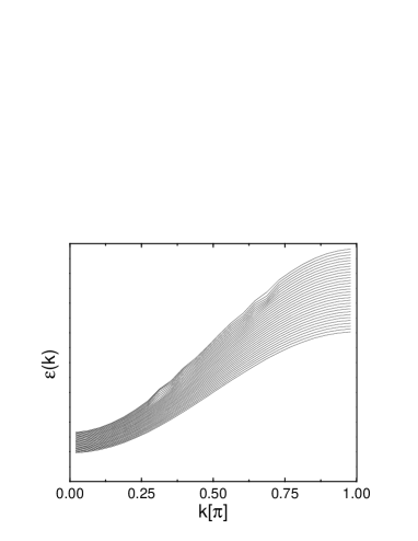
Figure 7: Renormalized dispersions from the CUT calculation for $N=48$. The results for $V=0.03,0.06,0.09\ldots,0.9$ are shifted with respect to each other in order to yield a three-dimensional view on the evolution of the dispersion.

At the end of the transformation, i.e. at $\ell=\infty$, when the effective hamiltonian has reached block diagonality only scattering processes are left which leave the number of quasi-particles unchanged. Then $\varepsilon_{k}$ is the renormalized 1-particle dispersion. This means that in the effective model after the transformation it is possible to add a single quasi-particle (hole or particle) to the ground state such that the resulting state is an exact eigen state because there is no other quasi-particle to interact with.

Note that this statement is not in contradiction with the widely known fact that the single-particle propagator $G(k,\omega)$ of a Luttinger liquid does not display quasi-particle peaks meden92 ; schon93 ; voit93a ; voit95 because the single-particle propagator $G(k,\omega)$ refers to adding or taking out a fermion before any transformation. It is an interesting issue, yet beyond the scope of the present work, to apply the CUT (3) to the creation and annihilation operators in order to recover the usual Luttinger liquid result in the framework of the CUT renormalization.

Fig. 7 shows the evolution of the dispersion for $N=48$ on increasing $V$. The dispersion behaves like a cosine-function with a renormalized Fermi velocity as expected from the exact result. For $V$ close to $V_{{\rm crit.}}(48)$ (at about $V=0.7$) there are kinks emerging. We reckon that these kinks represent spurious features induced by accumulated numerical inaccuracies for the same reasons for which the convergence is hampered for large system sizes.

Renormalized Fermi Velocity

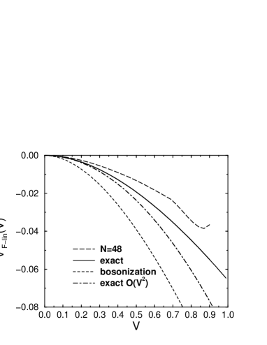
Figure 8: Comparison of the non-linear correlation part of the Fermi velocity as obtained for $N=48$ by the CUT with the exact thermodynamic result, the exact quadratic order $V^{2}$ and the result obtained from bosonization.

By fitting the function
$-v^{*}_{\rm F}\cos(k)$ to the calculated dispersions we obtain results for the renormalized Fermi velocity $v^{*}_{\rm F}$ as function of the interaction $V$. These values are dominated by the linear Fock term $1+\frac{2V}{\pi}$ or its finite-size equivalent in (14), respectively. In order to yield a better resolution of the influence of correlations we substract the constant and linear terms. The remainder $v^{*}_{\rm F-lin}$ is plotted in Fig. 8. It is compared to the exact result johns73 , the exact quadratic term $V^{2}$ and the result obtained from bosonization (cf. appendix C). The shape of the curves is basically the same. The CUT result is too small (in modulus) compared to the exact results. For small $V$ this is mainly due to a finite-size effect as comes out from an extrapolation $N\to\infty$. Again, the CUT approach is less reliable close to the critical interaction value $V_{\rm crit}(N)$.

Note that the bosonization results fits less well to the exact result than does the CUT result. This is due to the fact that in bosonization only the processes infinitely close to the Fermi points are considered. The deviation between the dash-dotted second order curve from the exact results reveals that higher order terms are important as well. They are partly captured by the CUT procedure.

3.5 Momentum Distribution

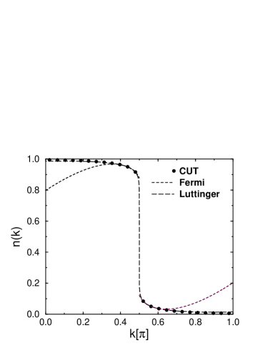
Figure 9: Momentum distribution as obtained by CUT for $V=0.6$ and 48 sites. Lines are interpolations to the three points closest to the Fermi wave vector assuming Luttinger (33) or Fermi behaviour (34), respectively.

Figure 10: Luttinger exponent $\alpha(V)$ as obtained from least-square fits of the CUT momentum distributions.

Last but not least we analyze the momentum distribution $n(k)$ in order to show that Luttinger liquid behaviour is retrieved. The standard approach to do so would be to transform the operator $c^{\dagger}_{k}c^{\phantom{\dagger}}_{k}$ according to Eq. (3) wegne94 ; hofst00 . Here, however, we use a simpler approach suitable for static expectation values and correlations. The value $E_{\infty}=E(\ell=\infty)$ is the ground state energy within our approximation because the block diagonal effective hamiltonian $H(\ell=\infty)$ does not contain processes exciting the vacuum any more. First order perturbation theory shows straightforwardly that functional derivation of $E_{\infty}$ yields the expectation value $n(k)$

$$\frac{dE_{\infty}}{d\varepsilon_{k}}=\left\langle\frac{dH}{d\varepsilon_{k}}\right\rangle=\langle:c^{\dagger}_{k}c^{\phantom{\dagger}}_{k}:\rangle=:n(k)\ .$$ (32)

In the numerical treatment the functional derivation can be easily realized by approximating the ratio of infinitesimal differences by the ratio of small finite differences. Hence no serious extension of the algorithm is needed to compute the momentum distribution. For relative variations of $\varepsilon_{k}$ around $10^{-3}$ the ground state energy $E_{\infty}$ is linear in these variations within an accuracy of about $10^{-5}$. So $n(k)$ can be determined to this accuracy. In Fig. 9 the momentum distribution (symbols) for $N=48$ and $V=0.6$ obtained in this way is depicted.

Due to the discretization $n(k)$ can be computed only for a finite set of points. At first sight, a jump seems to dominate at the Fermi wave vector $\pi/2$. But a discretized power law distribution displays also a jump – in particular if the exponent is small. In order to understand the nature of the distribution a quantitative analysis is required. Hence we fit the distribution obtained to two functions, one being appropriate for describing a Luttinger liquid halda81a ; voit95

$$\left|n(k)-\textstyle\frac{1}{2}\right|\approx C_{1}(\Delta k)^{\alpha}+C_{2}\Delta k$$ (33)

the other being appropriate for describing a Fermi liquid noack99

$$\left|n(k)-\textstyle\frac{1}{2}\right|\approx\frac{1+Z_{k_{\rm F}}}{2}+C_{1}\ln(\Delta k)\Delta k+C_{2}\Delta k$$ (34)

with $\Delta k:=|k-k_{\rm F}|$. For both possibilities three free parameters ($\alpha$, $C_{1}$, $C_{2}$ or $Z_{k_{\rm F}}$, $C_{1}$, $C_{2}$, respectively) are determined. In Fig. 9 the parameters are fixed to interpolate the three points closest to the Fermi wave vector. Another way is to perform a least-square fit; the resulting curves are shown in Fig. 3 in Ref. heidb02a . In both analyses, the qualitative result is the same. The Luttinger fit describes our data much better than the Fermi fit. We conclude that our data describes rather a power law behaviour than a jump. We cannot exclude, however, a behaviour comprising a power law behaviour and a jump. But there is no reason to believe that such a behaviour should occur.

Due to the small exponents $\alpha$ occurring and the restricted system sizes the power law cannot be distinguished reliably from a logarithmic behaviour or from a function of some logarithm in $|k-k_{\rm F}|$. Note, however, that the simple logarithm found in Ref. wegne94 is not likely to occur since we do not transform the observable in leading order only. Infinite orders of the interaction $V$ contribute to the ground state energy and hence to the derivative (32).

In order to push the analysis one step further we compare the exponent $\alpha$ resulting from the fits to the exact one. The points in the vicinity of the Fermi wave vector are more influenced by finite size effects schon96 . Eventually, we choose the exponents coming from least-square fits. In Fig. 10 they are compared to the exact values, to the second order result and to the values coming from the direct application of bosonization (cf. appendix C). Clearly, the CUT results agree very well with exact data for not too large values of $V<0.6$. From the comparison to the exact second order term $V^{2}$ one sees that the CUT data describes the full exact result better than the second order term alone. We infer that the CUT data reproduces the third order term also. This does not come as a surprise since we showed above that the ground state energy is exact including the $V^{3}$ term. Thus any quantity derived from it will also be exact in the same order. So the momentum distribution $n(k)$ and hence the exponent $\alpha$ have to be exact up to and including $V^{3}$.

The comparison to the bosonization result in Fig. 10 is also instructive. By construction the bosonization result captures only the physics in an infinitesimal vicinity of the Fermi points. There no umklapp scattering is possible as can be seen from Eq. (13) or from the analyses in Refs. shank91 ; shank01 (cf. discussion after Eq. (18)). For this reason, the bosonization fails to detect any precursor of the incipient phase transition to the CDW occurring at $V=1$. The dependence of the $\alpha$ obtained from bosonization is hence much smoother than the exact result. The CUT result includes scattering at all momenta. So precursors of the phase transition can be captured. Unfortunately, the breakdown of the approximation as used here makes further statements on the description of the phase transition impossible.

4 Discussion

4.1 Conclusions

We presented general arguments in favour for a renormalization treatment of interacting fermionic systems by means of a continuous unitary transformation (CUT). The precise choice of the unitary transformation, i.e. the choice of its infinitesimal generator, was motivated and the general properties of the transformation were elucidated. The method was illustrated for a model of one-dimensional, repulsively interacting fermions without spin at half-filling. The technical considerations for the explicit calculation were given. An important point was a consistent, non-redundant notation (18) which made the crucial cancellation between the Cooper pair and the zero sound channel manifest. Results were obtained for the correlation part of the ground state energy, for the 1-particle dispersion, for the 2-particle vertex function and for the static momentum distribution. The findings were compared to exact results as far as possible. The agreement was very good.

The CUT employed uses standard quasi-particles as elementary excitations. So it represents an explicit construction of Landau’s mapping of the non-interacting quasi-particles to the elementary excitations of the interacting system heidb02a . Note that the existence of such a smooth connection is not surprising since already the bosonization identity for fermionic field operators halda81b ; voit95 represents such a smooth link. In the continuum limit, a spinless model with or without interaction can be mapped to a single mode boson model with linear dispersion. Hence, it is possible to link the interacting model via the bosonic model to the non-interacting one (see also the remark on Kehrein’s results kehre99 ; kehre01 below). We take the success of our approach as corroborating (numeric) evidence that Landau’s mapping exists in one dimension. In particular, the numerical findings of the momentum distribution $n(k)$ indicate that important features of Luttinger liquids could be retrieved. Signatures of a Luttinger-type power law behaviour at the Fermi points were found, though hampered by the accessible restricted system sizes.

We are convinced that CUTs represent a powerful renormalization scheme for low-dimensional systems. Since no states are eliminated the effective hamiltonian obtained at the end of the CUT allows to compute spatial (shown here) and temporal correlations (for an example, see Ref. knett01b ) at small and at large wave vectors or excitation energies, respectively. So, in principle, no information is lost in the course of the renormalization, in contrast to, for instance, Wilson’s renormalization wilso75 . Of course, approximations which are necessary in practical calculation will introduce some uncertainties. Recent developments in renormalization approaches by integrating out degrees of freedom allow also to compute high energy features if the observables are equally subject to the flow, see for instance the appendix in Ref. salmh01 . A major advantage of the CUT approach is that no frequency dependence needs to be kept. This represents an important facilitation for the actual numerical realization of the renormalization.

4.2 Connections to other Work

Life-Time of Excitations

If a complete or partial diagonalization is obtained by a continuous unitary transformation the eigen values are by construction real. So the excitations are well-defined in energy and they do not display a finite life-time. This statement appears almost trivial if one bears in mind only the mathematical linear algebra. From the physics points of view, however, one might be surprised since one is used to that excitations, for instance quasi-particles, have a finite life-time in many-body systems. This comes about because no true eigen state are considered when an excitation of finite life-time is studied.

For instance, adding a fermion to the ground state of an interacting fermion system by application of a simple creation operator generically does not yield an eigen state but a sophisticated superposition of true eigen states. This looks as if the “true” fermion added decayed because its spectral function displays a peak of some finite width. Technically, one still uses the normal single-particle basis but the self-energy $\Sigma(k,\omega)$ acquires a finite imaginary part which represents the fact that the single fermion is coupled to states with one or more particle-hole pairs. One may view $\varepsilon_{k}+\Sigma(k,\omega)$ as an imaginary eigen value of the single particle state. But the single particle state is not an eigen state of the underlying hamiltonian.

The description using a unitary transformation designed to diagonalize the original hamiltonian is different from the standard approach in physics sketched above. One tries to find real eigen vectors and eigen values. Broad spectral functions do not occur because of imaginary eigen values but because of the superposition of eigen vectors. Kehrein and Mielke coined the expression that “the observables decay” and described the phenomenon in the context of dissipation kehre97 .

So it is not surprising that, after the CUT is applied to one-dimensional fermions, we find quasi-particles with infinite life-time. These are quasi-particles after the transformation. The fermion before the transformation will decay into states with additional excited particle-hole states. So there is no contradiction. In this context it is interesting to note that there is a formulation of diagrammatic perturbation theory which uses also infinite life-time excitations balia61a ; balia61b . In this formulation the fermionic one-particle states acquire a renormalized eigen energy due to the interaction. The change of the eigen energy $\varepsilon\to\varepsilon^{\prime}$ leads to a change in the occupation number $(1-\exp(-\beta(\varepsilon-\mu)))^{-1}\to(1-\exp(-\beta(\varepsilon^{\prime}-\mu)))^{-1})$ balia61a . So this approach corroborates that a description of the physics in terms of non-decaying quasi-particles is possible. The question how dynamic correlations can be described is not discussed in Refs. balia61a ; balia61b .

CUTs as Numerical Approach

While the present work was being finished White white02 proposed a numerical scheme which is very similar in spirit to what we did here. Besides discrete transformations which work less efficiently, a continuous unitary transformation is used with an infinitesimal generator with matrix elements

$$\eta_{ij}(\ell)=\frac{1}{E_{i}(\ell)-E_{j}(\ell)}H_{ij}(\ell)\ ,$$ (35)

where a 1-particle basis is used, i.e. a basis in which the 1-particle part of the hamiltonian is diagonal. The 1-particle eigen energies are given by $E_{i}$. The approach is applied to a small molecule, namely H₂O, and the ground state energy is computed very reliably by rotating the original ground state to a Fermi sea, i.e. the quasi-particle vacuum. That means that states which partially occupied $n\geq 0.5$ are mapped to filled states and states which are partially empty are mapped to empty states. This is what we did in our present work as well. So Ref. white02 provides an independent investigation of the power of continuous unitary transformations for a different fermionic system. In addition, it is investigated in Ref. white02 to eliminate a number of states which lie far off the Fermi level without diagonalizing the problem completely by the continuous transformation. The remaining effective problem, which is simplified considerably due to the reduction of the Hilbert space, is then solved by standard diagonalization algorithms, e.g. DMRG. Also this approach proved to be very powerful.

Choice of CUT

In Ref. wegne94 , Wegner investigated a one-dimensional $n$-orbital model in the continuum limit by a continuous unitary transformation. The main difference in the unitary transformation is the use of a generator different from the one in Eq. (6), namely

$$\eta=[H_{\rm D},H]$$ (36)

where $H_{\rm D}$ is the part of the Hamilton one wants to keep. The approach succeeded when $H_{\rm D}$ comprised all terms that do not change the number of quasi-particles. Hence this renormalizing scheme is very similar to the one used in the present work. It would be an interesting issue to compare both approaches quantitatively in a simple model. There are arguments in favour for both of the two approaches.

First, the choice (6) has the advantage that the kind of terms that are generated is restricted: the block band structure is preserved. Second, off-diagonal terms changing the number of quasi-particles are eliminated even if they are not accompanied by a change of the 1-particle energies, i.e. certain degeneracies are lifted. Third, a suppression of off-diagonal parts starts already linearly in the differences of the diagonal parts. A weakness of the choice (6) is given when there are scattering processes which increment the number of quasi-particles but decrease the 1-particle energies. In this case, the corresponding amplitudes are first enhanced before the decrease to the end of the transformation. Due to the necessary truncations it may be difficult to control the quality of the approximation during the stage of enhancement.

On the other side, the choice (36) is firstly very robust since off-diagonal terms are always suppressed due to the fact that the energy difference occurs squared wegne94 . Second, one does not need to know explicitly the eigen basis of $H_{\rm D}$. The squares are generated automatically by the double commutator when Eq. (36) is combined with Eq. (2). Yet these two commutators must also to be computed which might be tedious. Another weakness arises when large-scale degeneracies spoil the method by stopping the renormalization prematurely. For instance, the vanishing of $\eta$ implies the stop of the flow but guarantees only that there is a common basis set of $H_{\rm D}$ and $H$, not that $H$ is diagonal. So the conservation of the number of quasi-particles is not ensured by the choice (36).

Summarizing the comparison of the choices (6,36) we reckon that (6) works better if the number of excitations correlates well with the energy. If this is not the case, the robustness of (36) may be preferable. Note that there are still completely different generators conceivable grote02 . For example, one can use in a basis of 1-particle states

$$\eta_{ij}(\ell) = 0\quad\mbox{if}\ q_{i}=q_{j}$$

$$\eta_{ij}(\ell) = \mbox{sign}(E_{i}-E_{j})H_{ij}\quad\mbox{otherwise}$$ (37)

where in case of degeneracy $E_{i}=E_{j}$ the energy of the state with more excitations is assumed to be infinitesimally higher. Such an approach captures advantages of (6) while avoiding its disadvantage. Further investigations of these issues are certainly called for.

Fermionic Excitations

The fact that we treat a system of interacting one-dimensional fermions in its Luttinger liquid phase without using explicitly collective bosonic modes might be surprising. Yet it is not uncommon that an interacting system is suitably described (after certain transformations) by free or nearly free fermions. As an example we quote the work by Kehrein who succeeded to map a sine-Gordon model by a sequence of continuous transformations onto a model of free fermions kehre99 ; kehre01 . Indeed, Kehrein’s mapping accomplishes this aim for a broader range of parameters than previous renormalization treatments. The neglect of interactions between the excitations viewed as elementary is a fairly severe approximation for $\beta^{2}<4\pi$ where the breathers, i.e. bound states, are known to occur bergk79 . Their description requires the inclusion of the interaction between elementary excitations.

Landau’s Fermi Liquid

Finally, we wish to comment on the use of a Landau’s Fermi liquid description in terms of quasi-particles for one-dimensional systems heidb02a . The possibility and the power of such a description has been noted previously by Carmelo et al. carme in the framework of the Bethe ansatz solution of the one-dimensional Hubbard model. Carmelo and coworkers use the spinons and holons as they arise in the Bethe ansatz solution as pseudo-particles. Then an approximate treatment for the spatial and temporal carme00 correlations is built by describing the excitations as small deviations from the ground state distributions of these pseudo-particles. In this sense, the concept of Landau’s Fermi liquid is generalized to one dimension. The author emphasize, however, that the pseudo-particles cannot be smoothly linked to the quasi-particles of the non-interacting solution. In this point, a clear difference to our finding here and in Ref. heidb02a occurs. We argue on the basis of our numerical results that a smooth mapping between the interacting and the non-interacting excitations exists even in one dimension. The existence of such a mapping as long as the system remains massless can already be deduced from bosonization. Since the interacting and the non-interacting model can be mapped to a model of free linear dispersion bosons (discarding Umklapp scattering) they can also be mapped to each other. By means of the CUT we constructed such a mapping explicitly.

The generalized Landau liquid in Refs. carme relies on the Bethe ansatz solution of the one-dimensional Hubbard model. Hence it may be that the integrability is a prerequisite for the generalized Landau liquid. In our calculation in contrast, the integrability of the model studied does not play a rôle other than providing a rigorous benchmark. But so far, we have not considered the spinful case. Its investigation by CUTs is certainly called for.

4.3 Outlook

A comprehensive summary is given in Sect. 4.1. Here we point out in which directions further work is required. In view of the numerical nature of the present work, an analytical treatment would be helpful. There is still a certain gap between the analytical result of a logarithmic divergence for the momentum distribution obtained in Ref. wegne94 and the numerical results we found. For an analytical treatment the models to be considered have to be simplified further. Spin, however, should be included in order to enlarge decisively the class of systems which can be described.

Another very interesting issue is the computation of dynamical quantities like the local spectral function $A(\omega)$ or the momentum resolved spectral function $A(k,\omega)$. In the framework of standard renormalization such investigations are presently carried out busch02 . The dynamical quantities are of interest to see theoretically to which extent and to which accuracy they can be computed at all energies and momenta. For the explanation of experimental data the spectral functions are of utmost importance. It is this objective which requires in particular to go beyond the asymptotic regime of very small energies and momenta claes02 . For gapful spin systems dynamical quantities have already been computed successfully knett01b . The results agree very well with experiments and render deeper insight in the underlying physics windt01 ; schmi01 .

In order to go beyond one-dimensional systems, modified generators have to be investigated, see e.g. grote02 . The pros and cons of the choices used presently were briefly discussed in the preceding section. The issue of the optimum generator represents a longer-lasting question since the answer depends certainly on the model to be studied.

Acknowledgements

It is a pleasure for us to acknowledge interesting and helpful discussions with N. Grewe, S. Kehrein, P. Horsch, E. Müller-Hartmann, M. Salmhofer, S.R. White and P. Wölfle. This work has been supported by the Deutsche Forschungsgemeinschaft through SP 1073 and through SFB 608.

Appendix A Normal-Ordering

Normal-ordering wick50 denoted by colons $:A:$ is a standard procedure which is explained at length in the text books negel88 . So we recall here only the gist of it which is technically relevant for our calculation. For further details we refer the reader to the concise script by Wegner wegne00 .

Considering a product $X_{n}$ of $n$ fermionic operators it is a priori not clear on how many particles this operator really acts. It looks as if it acted on $n$ fermions. But a part of this action may be redundant in the sense that it can be expressed also by an operator $Y_{m}$ with $m<n$. This is indeed the generic situation. A point of reference is needed in order to be able to define how many particles are involved in a certain process. Given the ground state of a 1-particle hamiltonian the normal-ordering ensures that the normal-ordered $n$ operator does not contain parts which can be viewed as action of an operator with less fermionic factors. This is the physical content of

$$\langle:P_{n}::Q_{m}:\rangle=0\quad\mbox{for}\quad n\neq m\$$ (38)

as derived for normal-ordered terms wegne00 .

Technically, a usual product of $m$ fermionic operators $a_{k}$ is expressed in terms of normal-ordered terms as

$$a_{k1}a_{k2}\ldots a_{km}=$$

$$\quad:\exp\left(\sum_{k,l}G_{kl}\textstyle\frac{\partial^{2}}{\partial a_{l}^{\rm right}\partial a_{l}^{\rm left}}\right)a_{k1}a_{k2}\ldots a_{km}:\ ,\quad$$ (39)

where $G_{kl}$ is the contraction $\langle a_{k}a_{l}\rangle$. The superscripts ‘left’ and ‘right’ indicate that in the double derivatives only pairs are taken where $a^{\rm left}_{k}$ is a factor to the left of $a^{\rm right}_{l}$. To obtain the correct signs the ‘left’ derivation must be taken before the ‘right’ excitation. Eq. (39) stands for the known procedure that a product is normal ordered by writing down the sum of terms with all possible numbers and sorts of contractions. The inverse relation is given simply by

$$:a_{k1}a_{k2}\ldots a_{km}:=$$

$$\quad\exp\left(-\sum_{k,l}G_{kl}\textstyle\frac{\partial^{2}}{\partial a_{l}^{\rm right}\partial a_{l}^{\rm left}}\right)a_{k1}a_{k2}\ldots a_{km}\ .\quad$$ (40)

Combining Eqs. (39) and (40) leads to the useful expression for products of normal-ordered terms $:A(a):$ and $:B(a):$

$$:A(a)::B(a):=:\exp\left(\sum_{k,l}G_{kl}\textstyle\frac{\partial^{2}}{\partial b_{l}\partial a_{l}}\right)A(a)B(b):\Big{|}_{b=a}$$ (41)

where the superscripts ‘left’ and ‘right’ are no longer needed due to the sequence of factors in the product. In practice, Eq. (41) means that for the normal-ordering of a product of already normal-ordered factors not all contractions need to be considered. Only those contractions matter where the two fermionic operator do not come from the same factor. This is easy to understand since the contractions between fermionic operators from the same factor are already accounted for by the normal-ordering of each factor separately.

In order to determine the differential equations resulting from Eq. (2) commutators of normal-ordered terms must be computed. To do this without passing by non-normal-ordered expressions an extension of Eq. (41) to commutators is particularly useful. We derived and checked the identity

$$[:A(a):,:B(a):]=$$

$$\qquad:\exp\left(\sum_{k,l}G_{kl}\left(\textstyle\frac{\partial^{2}}{\partial a_{l}^{\rm right}\partial b_{k}^{\rm left}}+\textstyle\frac{\partial^{2}}{\partial b_{l}^{\rm right}\partial a_{k}^{\rm left}}\right)\right)$$

$$\qquad\qquad[A(a),B(b)]:\Big{|}_{b=a}\ ,\quad$$ (42)

where the commutator is computed using the anticommutators $\{a_{k},b_{l}\}:=\{a_{k},a_{l}\}$. Eq. (42) means that one can first compute the commutator as usual, but remembering whether the fermionic operator comes from $A$ or from $B$. Then normal-ordering is achieved by writing down the terms with all possible contractions between pairs of fermionic operators where one comes from $A$ and the other from $B$. In this way, the computation of the actual general flow equation (2) becomes a task which is not too demanding.

Appendix B The Self-Similar CUTs

In the self-similar approxmation we compute

$$\left[T^{(0)}_{0}(\ell)+T^{(1)}_{0}(\ell)+\sum^{+2}_{-2}T^{(2)}_{2i}(\ell),\sum^{+2}_{-2}\mbox{sign}(i)T^{(2)}_{2i}(\ell)\right]$$ (43)

neglecting the arising $T^{(3)}_{i}$ terms. The change in the number of quasi-particles for the expression
$\Gamma_{kqp}:c^{\dagger}_{k+q}c^{\dagger}_{k-q}c^{\phantom{\dagger}}_{k-p}c^{\phantom{\dagger}}_{k+p}:$ is given by $S_{kqp}$ as defined by

$$S_{kqp} = \mbox{sign}(n_{k+p}+n_{k-p}-n_{k-q}-n_{k+q})\ ,$$ (44)

where we use $n_{k}$ for the momentum distribution of the unperturbed Fermi sea since this is the quasi-particle vacuum to which we are mapping the ground state. (The actual momentum distribution is denoted $n(k)$). With these definitions we calculate the commutator using normal-ordering as explained in appendix A. Then we compare the coefficients of the various terms (0-particle, 1-particle and 2-particle terms) and determine in this way the set of differential equations.

B.1 Ground state energy per site

The differential equation of the ground state energy per site depends only on the commutator $[T^{(2)}_{\pm 4},T^{(2)}_{\mp 4}]$ where all fermionic operators are contracted. There are four different ways to combine the operators for the complete contractions. But all of them lead to the same expression if one uses the symmetries Eq.(15)-(18). Finally one obtains

$$\frac{d}{dl}\frac{E}{N}=\frac{8}{N^{3}}\!\!\!\!\sum_{{k\in[0,\pi)}\atop{qp\in[-\pi,\pi)}}\!\!\!\!(1-2\,n_{k+p})\,n_{k+q}\,n_{k-q}\,S_{k,q,p}\,{\Gamma_{k,q,p}^{2}}.\qquad$$ (45)

B.2 Dispersion

For the 1-particle term, the dispersion, one has to take all combinations of three contractions into account that occur in $[T^{(2})_{i},T^{(2)}_{-i}]$ with $i\in\{0,\pm 2,\pm 4\}$. One obtains $16$ different parts that turn out to be identical. In order to avoid double-counting one of the free momenta must be restricted to $[0,\pi)$ or the sum must be divided by two. So one obtains finally

$$\frac{d}{dl}\varepsilon_{k}=$$

$$\quad\frac{8}{N^{2}}\!\!\!\!\sum_{qp\in[-\pi,\pi)}\!\!\!\!((1-2n_{k+q-p})n_{k-2q}+n_{n+p-q}n_{n-p-q})\times$$

$$\qquad S_{k-qqp}\Gamma^{2}_{k-qqp}\ .$$ (46)

B.3 Vertex Function

For the vertex function $\Gamma_{kqp}$ there are two commutators to calculate: $[T^{(2)}_{i},T^{(2)}_{j}]$ ($i,j\in\{0,\pm 2,\pm 4\}$) with all possible combinations of two contractions and $[T^{(1)}_{0},T^{(2)}_{j}]$ with all possibilities of a single contraction. To keep the notation short, we define

$$\Phi_{kqp|KQP}:=(S_{kqp}-S_{KQP})\Gamma_{kqp}\Gamma_{KQP}\ .$$ (47)

The differential equation for the flow of $\Gamma_{kqp}$ then reads

$$\frac{d}{dl}\Gamma_{kqp}=(\varepsilon_{k+p}+\varepsilon_{k-p}-\varepsilon_{k-q}-\varepsilon_{k+q})S_{kqp}\Gamma_{kqp}+$$

$$\quad\frac{1}{N}\sum_{Q\in[-\pi,\pi)}4n_{Q}\Big{\{}$$

$$\quad\Phi_{\frac{k+q+Q}{2}\frac{k+q-Q}{2}\frac{k-q-Q}{2}-p|\frac{k+p+Q}{2}\frac{k-p-Q}{2}-q\frac{k+p-Q}{2}}+$$

$$\quad\Phi_{\frac{k-q+Q}{2}\frac{k-q-Q}{2}\frac{k+q-Q}{2}+p|\frac{k-p+Q}{2}\frac{k+p-Q}{2}+q\frac{k-p-Q}{2}}-$$

$$\quad\Phi_{\frac{k+q+Q}{2}\frac{k+q-Q}{2}\frac{k-q-Q}{2}+p|\frac{k-p+Q}{2}\frac{k+p-Q}{2}-q\frac{k-p-Q}{2}}-$$

$$\quad\Phi_{\frac{k-q+Q}{2}\frac{k-q-Q}{2}\frac{k+q-Q}{2}-p|\frac{k+p+Q}{2}\frac{k-p-Q}{2}+q\frac{k+p-Q}{2}}$$

$$\quad\Big{\}}+2(1-2n_{Q})\Phi_{kq(Q-k)|k(Q-k)p}\ .$$ (48)

Note that the appearance of four $\Phi$-terms is due to the fact that we denote the scattering processes in the hamiltonian (1) in a notation symmetric way (18). A naive comparison of coefficients would lead only to one of the four terms. The other three come into play if one requires that $\frac{d}{dl}\Gamma_{kqp}$ fulfills (18). As explained in the main text, the notation obeying (18) ensures that a maximum number of cancellations are dealt with explicitly. This is advantageous on the numerical as well as on the conceptual level.

Appendix C Bosonization of the Model

We employ a constructive bosonization by linearizing the dispersion on both branches ($r=+1\leftrightarrow$ right branch, $r=-1\leftrightarrow$ left branch)

$$\varepsilon_{k,r}=r\left(1+\textstyle\frac{2V}{\pi}\right)(k-rk_{\rm F})\ .$$ (49)

Furthermore, the bare interaction vertex (13) is evaluated with all momenta being taken at the Fermi points $\pm k_{\rm F}$. The corresponding scattering strengths take the value $\pm V$. Following Ref. voit95 one can then determine the renormalized Fermi velocity as

$$v^{*}_{\rm F}(V)=\left(1+\textstyle\frac{2V}{\pi}\right)\sqrt{1-\left(\textstyle\frac{2V}{\pi+2V}\right)^{2}}$$ (50)

and the exponent $\alpha$ occurring in the momentum distribution from Eq. (22) and

$$\eta_{0}(V) = \frac{1}{2}\sqrt{\frac{2\pi}{2\pi+8V}}\ .$$ (51)

References

- (1) J. G. Bednorz and K. A. Müller, Z. Phys. B 64, 189 (1986).
- (2) P. W. Anderson, The Theory of Superconductivity in the High- Cuprate Superconductors (Princeton University Press, New Jersey, 1997).
- (3) E. W. Carlson, V. J. Emery, S. A. Kivelson, and D. Orgad, in The Physics of Conventional and Unconventional Superconductors (Springer-Verlag, Heidelberg, 2002).
- (4) K. G. Wilson, Rev. Mod. Phys. 47, 773 (1975).
- (5) R. Shankar, Rev. Mod. Phys. 66, 129 (1994).
- (6) D. Zanchi and H. J. Schulz, Z. Phys. B 103, 339 (1997).
- (7) C. J. Halboth and W. Metzner, Phys. Rev. B 61, 7364 (2000).
- (8) C. Honerkamp, M. Salmhofer, N. Furukawa, and T. M. Rice, Phys. Rev. B 63, 035109 (2001).
- (9) V. Meden, W. Metzner, U. Schollwöck, and K. Schönhammer, J. Low Temp. Phys. 126, 1147 (2002).
- (10) F. J. Wegner, Ann. Physik 3, 77 (1994).
- (11) S. D. Głazeck and K. G. Wilson, Phys. Rev. D 48, 5863 (1993).
- (12) S. D. Głazeck and K. G. Wilson, Phys. Rev. D 49, 4214 (1994).
- (13) C. P. Heidbrink and G. S. Uhrig, Phys. Rev. Lett. 88, 146401 (2002).
- (14) C. Knetter, K. P. Schmidt, M. Grüninger, and G. S. Uhrig, Phys. Rev. Lett. 87, 167204 (2001).
- (15) S. R. White, J. Chem. Phys. 117, 7472 (2002).
- (16) P. Nozières, Theory of Interacting Fermi Systems (Addison-Wesley, Reading, Massachusetts, 1997).
- (17) J. Voit, Rep. Prog. Phys. 58, 977 (1995).
- (18) A. O. Gogolin, A. A. Nersesyan, and A. M. Tsvelik, Bosonization and Strongly Correlated Systems (Cambridge University Press, Cambridge, UK, 1998).
- (19) J. Feldman, D. Lehmann, H. Knörrer, and E. Trubowitz, in Constructive Physics, Vol. 446 of Lecture Notes in Physics, edited by V. Rivasseau (Springer, Heidelberg, 1995), p. 267.
- (20) A. Mielke, Eur. Phys. J. B 5, 605 (1998).
- (21) C. Knetter and G. S. Uhrig, Eur. Phys. J. B 13, 209 (2000).
- (22) C. Knetter, A. Bühler, E. Müller-Hartmann, and G. S. Uhrig, Phys. Rev. Lett. 85, 3958 (2000).
- (23) F. D. M. Haldane, J. Phys. C14, 2585 (1981).
- (24) E. Fradkin, Field Theories of Condensed Matter Systems, Vol. 82 of Lecture Annote Series (Addison Wesley, Redwood City, 1991).
- (25) B. Joós, T. L. Einstein, and N. C. Bartelt, Phys. Rev. B 43, 8153 (1991).
- (26) H. Bethe, Z. Phys. 71, 205 (1931).
- (27) C. N. Yang and C. P. Yang, Phys. Rev. 150, 321 and 327 (1966).
- (28) C. N. Yang and C. P. Yang, Phys. Rev. 151, 258 (1966).
- (29) J. D. Johnson, S. Krinsky, and B. M. McCoy, Phys. Rev. A 8, 2526 (1973).
- (30) A. Luther and I. Peschel, Phys. Rev. B 12, 3908 (1975).
- (31) F. D. M. Haldane, Phys. Rev. Lett. 45, 1358 (1980).
- (32) F. D. M. Haldane, Phys. Rev. Lett. 47, 1840 (1981).
- (33) R. Shankar, Physica A177, 530 (1991).
- (34) R. Shankar, J. Stat. Phys. 103, 485 (2001).
- (35) V. Meden and K. Schönhammer, Phys. Rev. B 46, 15753 (1992).
- (36) C. P. Heidbrink, Flussgleichungsrenormierung eines spinlosen eindimensionalen Fermisystems (Diplomarbeit, Köln, 2001).
- (37) J. Sólyom, Adv. Phys. 28, 201 (1979).
- (38) K. Schönhammer and V. Meden, Phys. Rev. B 47, 16205 (1993).
- (39) J. Voit, Phys. Rev. B 47, 6740 (1993).
- (40) W. Hofstetter, Renormalization Group Methods for Quantum Impurity Systems (Verlag Shaker, Aachen, 2000).
- (41) R. M. Noack and F. Gebhard, Phys. Rev. Lett. 82, 1915 (1999).
- (42) K. Schönhammer and V. Meden, Am. J. Phys. 64, 1168 (1996).
- (43) S. Kehrein, Phys. Rev. Lett. 83, 4914 (1999).
- (44) S. Kehrein, Nucl. Phys. B 592, 512 (2001).
- (45) M. Salmhofer and C. Honerkamp, Prog. Theor. Phys. 105, 1 (2001).
- (46) S. K. Kehrein and A. Mielke, Ann. Physik 6, 90 (1997).
- (47) R. Balian, C. Bloch, and C. de Dominicis, Nucl. Phys. 25, 529 (1961).
- (48) R. Balian, C. Bloch, and C. de Dominicis, Nucl. Phys. 27, 294 (1961).
- (49) I. Grote, E. Körding, and F. Wegner, J. Low Temp. Phys. 126, 1385 (2002).
- (50) H. Bergknoff and H. B. Thacker, Phys. Rev. D 19, 3666 (1979).
- (51) J. M. P. Carmelo and A. A. Ovchinnikov, J. Phys.: Condens. Matter 3, 757 (1991); J. M. P. Carmelo and P. Horsch, Phys. Rev. Lett. 68, 871 (1992); J. M. P. Carmelo, P. Horsch, and A. A. Ovchinnikov, Phys. Rev. B 45, 7899 (1992); ibid., Phys. Rev. B 46, 14728 (1992).
- (52) J. M. P. Carmelo, N. M. R. Peres, and P. D. Sacramento, Phys. Rev. Lett. 84, 4673 (2000).
- (53) T. Busche, L. Bartosch, and P. Kopietz, cond-mat/0202175 (2002).
- (54) R. Claessen et al., Phys. Rev. Lett. 88, 096402 (2002).
- (55) M. Windt et al., Phys. Rev. Lett. 87, 127002 (2001).
- (56) K. P. Schmidt, C. Knetter, and G. S. Uhrig, Europhys. Lett. 56, 877 (2001).
- (57) G. C. Wick, Phys. Rev. 80, 268 (1950).
- (58) J. W. Negele and H. Orland, Quantum Many-Particle Systems, Vol. 68 of Frontiers in Physics (Addison Wesley, Redwood City, 1988).
- (59) F. J. Wegner, http://www.tphys.uni-heidelberg.de/~wegner/, Skripten: Zum Wick-Theorem und zur Normal-Ordnung.