Renormalized perturbation theory for Fermi systems:
Fermi surface deformation and superconductivity in the two-dimensional Hubbard model

Abstract

Divergencies appearing in perturbation expansions of interacting many-body systems can often be removed by expanding around a suitably chosen renormalized (instead of the non-interacting) Hamiltonian. We describe such a renormalized perturbation expansion for interacting Fermi systems, which treats Fermi surface shifts and superconductivity with an arbitrary gap function via additive counterterms. The expansion is formulated explicitly for the Hubbard model to second order in the interaction. Numerical solutions of the self-consistency condition determining the Fermi surface and the gap function are calculated for the two-dimensional case. For the repulsive Hubbard model close to half-filling we find a superconducting state with d-wave symmetry, as expected. For Fermi levels close to the van Hove singularity a Pomeranchuk instability leads to Fermi surfaces with broken square lattice symmetry, whose topology can be closed or open. For the attractive Hubbard model the second order calculation yields s-wave superconductivity with a weakly momentum dependent gap, whose size is reduced compared to the mean-field result.

PACS: 71.10.Fd, 71.10.-w, 74.20.Mn

I Introduction

Unrenormalized perturbation expansions of interacting electron systems around the non-interacting part of the Hamiltonian are generally plagued by infrared divergencies. Some of the divergencies are simply due to to shifts of the Fermi surface, while others signal instabilities of the normal Fermi liquid towards qualitatively different states, such as superconducting or other ordered phases. This problem is often treated by self-consistent resummations of Feynman diagrams, where a finite or infinite subset of skeleton diagrams, with the interacting propagator $G$ on internal lines, is summed.[1] Symmetry breaking can be built into the structure of $G$ as an ansatz, and the size of the corresponding order parameter is determined self-consistently. This standard approach has been very useful in many cases. However, resummation schemes beyond first order (Hartree-Fock) require extensive numerics, since the full self-energy has to be determined self-consistently, and delicate low-energy structures cannot always be resolved. A more serious problem is the fact that self-energy and vertex corrections are not treated on equal footing in most feasible resummation schemes. This often leads to unphysical results.

In this work we will describe and apply an alternative procedure, which has been formulated already long ago by Nozières,[2] and more recently been discussed in the mathematical literature as a way of carrying out well-defined perturbation expansions for weakly interacting Fermi systems.[3, 4] The basic idea is to choose an improved starting point for the perturbation expansion, by adding a suitable counterterm to the non-interacting part of the Hamiltonian, and subtracting it from the interaction part. The counterterm is quadratic in the Fermi operators and has to be determined from a self-consistency condition. In Sec. II we will describe how Fermi surface deformations and superconductivity can be treated by this method. Explicit expressions up to second order in the interaction are derived for the case of the Hubbard model in Sec. III. Results obtained from a numerical solution of the self-consistency equations in two dimensions will follow in Sec. IV. For the repulsive Hubbard model we have obtained superconducting solutions with d-wave symmetry in agreement with widespread expectations,[5] and with recent renormalization group calculations which conclusively established d-wave superconductivity at weak coupling.[6] In addition, for Fermi levels close to the van Hove singularity, deformations which break the square lattice symmetry occur. This confirms the recently proposed possibility of symmetry-breaking Fermi surface deformations (”Pomeranchuk instabilities”).[7, 8, 9]

II Renormalized perturbation expansion

We consider a system of interacting spin-$\frac{1}{2}$ fermions with a Hamiltonian $H=H_{0}+H_{I}$, where the non-interacting part

$$H_{0}=\sum_{{\bf k},\sigma}\xi_{{\bf k}}\,n_{{\bf k}\sigma}$$ (1)

with $\xi_{{\bf k}}=\epsilon_{{\bf k}}-\mu$ contains the kinetic energy and the chemical potential, while $H_{I}$ is a fermion-fermion interaction term. We are particularly interested in lattice systems, for which the dispersion relation $\epsilon_{{\bf k}}$ is not isotropic. We consider only ground state properties, that is the temperature is zero throughout the whole article.

The bare propagator in a standard many-body perturbation expansion [10] around $H_{0}$ is given by

$$G_{0}(k)=\frac{1}{i\omega-\xi_{{\bf k}}}\;,$$ (2)

where $\omega$ is the Matsubara frequency and $k=(\omega,{\bf k})$. This progagator diverges for $\omega\to 0$ and ${\bf k}\to{\bf k}_{F}$, for any Fermi momentum ${\bf k}_{F}$, since $\xi_{{\bf k}_{F}}=0$. As a consequence, many Feynman diagrams diverge. A well-known singularity is the (usually) logarithmic divergency of the 1-loop particle-particle contribution to the two-particle vertex in the Cooper channel, which leads to a $(\log)^{n}$ divergency of the n-loop particle-particle ladder diagram. This signals a possible Cooper instability towards superconductivity. Much stronger divergencies occur in diagrams with multiple self-energy insertions on the same internal propagator line, leading to non-integrable powers of $G_{0}(k)$.[3, 4] These singularities are due to Fermi surface shifts generated by the interaction term in the Hamiltonian.

The divergency problems and the superconducting instability can be treated by splitting the Hamiltonian in a different way, namely as[2]

$$H=\tilde{H}_{0}+\tilde{H}_{I}\;,$$ (3)

where $\tilde{H}_{0}=H_{0}+\delta H_{0}$ and $\tilde{H}_{I}=H_{I}-\delta H_{0}$, and expanding around $\tilde{H}_{0}$. The counterterm $\delta H_{0}$ must be quadratic in the creation and annihilation operators to allow for a straightforward perturbation expansion based on Wick’s theorem. It is possible to chose $\delta H_{0}$ such that $\tilde{H}_{I}$ does not shift the Fermi surface corresponding to $\tilde{H}_{0}$ any more, and divergencies due to self-energy insertions are removed. In the superconducting state spontaneous symmetry breaking can be included already in $\delta H_{0}$, with an order parameter $\Delta_{{\bf k}}$ whose value on the Fermi surface is not shifted by $\tilde{H}_{I}$. We will now describe this procedure in more detail.

A Normal state

A counterterm $\delta H_{0}=\sum_{{\bf k},\sigma}\delta\xi_{{\bf k}}\,n_{{\bf k}\sigma}$ leads to a renormalized dispersion relation $\tilde{\xi}_{{\bf k}}=\xi_{{\bf k}}+\delta\xi_{{\bf k}}$ in the unperturbed part of the Hamiltonian,

$$\tilde{H}_{0}=\sum_{{\bf k},\sigma}\tilde{\xi}_{{\bf k}}\,n_{{\bf k}\sigma}\;,$$ (4)

and correspondingly to a new bare propagator

$$\tilde{G}_{0}(k)=\frac{1}{i\omega-\tilde{\xi}_{{\bf k}}}\;.$$ (5)

The Fermi surface $\tilde{\cal F}$ associated with $\tilde{H}_{0}$ is given by the momenta $\tilde{\bf k}_{F}$ satisfying the equation $\tilde{\xi}_{{\bf k}}=0$. The Fermi surface of the interacting system is given by the solutions of the equation $G^{-1}(0,{\bf k})=0$. This surface coincides with the unperturbed one, corresponding to $\tilde{H}_{0}$, if the renormalized self-energy $\tilde{\Sigma}=\tilde{G}_{0}^{-1}-G^{-1}$ vanishes on $\tilde{\cal F}$, that is if

$$\tilde{\Sigma}(0,{\bf k})=0\quad\mbox{for}\quad{\bf k}\in{\tilde{\cal F}}\;.$$ (6)

This imposes a self-consistency condition on the counterterms which can be solved iteratively. For isotropic systems the shift of $\xi_{{\bf k}}$ can be chosen as a momentum independent constant, which may be interpreted as a shift of the chemical potential. For anisotropic systems, however, one generally has to adjust the whole shape of the Fermi surface. That this procedure really works at each order of the perturbation expansion has been shown rigorously for a large class of systems.[11]

The shift function $\delta\xi_{{\bf k}}$ is uniquely determined by the self-consistency condition only on the (interacting) Fermi surface $\tilde{\cal F}$. For momenta away from the Fermi surface, $\delta\xi_{{\bf k}}$ can be chosen to be any sufficiently smooth function of ${\bf k}$ which does not lead to artificial additional zeros of $\tilde{\xi}_{{\bf k}}$.

The perturbation expansion of the renormalized self-energy $\tilde{\Sigma}$ involves two types of vertices: the usual two-particle vertex given by the interaction $H_{I}$ and a one-particle vertex due to the counterterm $-\delta H_{0}$ in $\tilde{H}_{I}$. In Fig. 1 we show the Feynman diagrams contributing to $\tilde{\Sigma}$ up to second order in the interaction.

The above-mentioned divergencies of Feynman diagrams with self-energy insertions on internal propagator lines are removed in the renormalized expansion around $\tilde{H}_{0}$, since in products $\tilde{G}_{0}\tilde{\Sigma}\tilde{G}_{0}\dots\tilde{\Sigma}\tilde{G}_{0}$ only one simple pole at $k=(0,\tilde{\bf k}_{F})$ survives, all other poles being cancelled by the corresponding zeros of the self-energy $\tilde{\Sigma}$.

B Superconducting state

To treat superconducting states we also add counterterms containing Cooper pair creation and annihilation operators, in addition to a shift of $\xi_{{\bf k}}$. We consider only spin singlet pairing, but triplet pairing could be dealt with analogously. We thus expand around a BCS mean-field Hamiltonian

$$\tilde{H}_{0}=\sum_{{\bf k},\sigma}\tilde{\xi}_{{\bf k}}\,n_{{\bf k}\sigma}+\sum_{{\bf k}}\left[\Delta_{{\bf k}}\,a^{{\dagger}}_{-{\bf k}\downarrow}a^{{\dagger}}_{{\bf k}\uparrow}+\Delta^{*}_{{\bf k}}\,a_{{\bf k}\uparrow}a_{-{\bf k}\downarrow}\right]\;,$$ (7)

where $\Delta_{{\bf k}}$ is the gap-function, which has to be determined self-consistently. In terms of Nambu operators

$$\Psi_{{\bf k}}=\left(\begin{array}[]{l}a_{{\bf k}\uparrow}\\ a^{{\dagger}}_{-{\bf k}\downarrow}\end{array}\right)\quad\mbox{and}\quad\Psi^{{\dagger}}_{{\bf k}}=\left(a^{{\dagger}}_{{\bf k}\uparrow}\,,\,a_{-{\bf k}\downarrow}\right)$$ (8)

one can rewrite $\tilde{H}_{0}$ in more compact form as

$$\tilde{H}_{0}=\sum_{{\bf k}}\tilde{\xi}_{{\bf k}}\,\Psi^{{\dagger}}_{{\bf k}}\,\sigma_{3}\,\Psi_{{\bf k}}-\sum_{{\bf k}}\Psi^{{\dagger}}_{{\bf k}}\,(\Delta^{\prime}_{{\bf k}}\,\sigma_{1}-\Delta^{\prime\prime}_{{\bf k}}\,\sigma_{2})\,\Psi_{{\bf k}}\;,$$ (9)

where $\sigma_{1},\sigma_{2},\sigma_{3}$ are the Pauli matrices, and $\Delta^{\prime}_{{\bf k}}$ ($\Delta^{\prime\prime}_{{\bf k}}$) is the real (imaginary) part of $\Delta_{{\bf k}}$. The two expressions (7) and (9) for $\tilde{H}_{0}$ differ by the constant (c-number) $\sum_{{\bf k}}\tilde{\xi}_{{\bf k}}$, which must be taken into account only when absolute energies are computed. The bare Nambu matrix propagator ${\bf\tilde{G}}_{0}=-\langle\Psi\Psi^{{\dagger}}\rangle_{\tilde{0}}$ following from $\tilde{H}_{0}$ is given by

$${\bf\tilde{G}}_{0}^{-1}(k)=\left(\begin{array}[]{cc}i\omega-\tilde{\xi}_{{\bf k}}&\Delta_{{\bf k}}\\ \Delta^{*}_{{\bf k}}&i\omega+\tilde{\xi}_{{\bf k}}\end{array}\right)\;.$$ (10)

Extending the self-consistency condition for the normal state, we now require that the matrix self-energy ${\boldsymbol{\tilde{\Sigma}}}={\bf\tilde{G}}_{0}^{-1}-{\bf G}^{-1}$ vanishes on the Fermi surface (defined by $\tilde{\xi}_{{\bf k}}=0$), that is

$${\boldsymbol{\tilde{\Sigma}}}(0,{\bf k})=0\quad\mbox{for}\quad{\bf k}\in{\tilde{\cal F}}\;.$$ (11)

Thus, for $\omega=0$ and ${\bf k}$ on the Fermi surface, neither the diagonal nor the off-diagonal elements of ${\bf\tilde{G}}_{0}^{-1}(k)$ are shifted by the interaction term $\tilde{H}_{I}$. The Feynman diagrams in Fig. 1 apply also to the superconducting case, if lines are interpreted as Nambu matrix propagators.

The above renormalized perturbation theory is reminiscent of the perturbation theory for symmetry broken phases formulated by Georges and Yedidia,[12] where an order-parameter-dependent free energy function is constructed by adding Onsager reaction terms to the mean field contributions, and the actual order parameter is determined by minimizing this free energy.

III Application to the Hubbard model

In this section we derive explicit expressions for the self-energy and the counterterms for the ground state $(T=0)$ of the Hubbard model, up to second order in the renormalized perturbation expansion.

The one-band Hubbard model [13]

$$H=\sum_{{\bf i},{\bf j}}\sum_{\sigma}t_{{\bf i}{\bf j}}\,c^{{\dagger}}_{{\bf i}\sigma}c_{{\bf j}\sigma}+U\sum_{{\bf j}}n_{{\bf j}\uparrow}n_{{\bf j}\downarrow}-\mu N$$ (12)

describes lattice electrons with a hopping amplitude $t_{{\bf i}{\bf j}}$ and a local interaction $U$. Here $c^{{\dagger}}_{{\bf i}\sigma}$ and $c_{{\bf i}\sigma}$ are creation and annihilation operators for electrons with spin projection $\sigma$ on a lattice site ${\bf i}$, and $n_{{\bf j}\sigma}=c^{{\dagger}}_{{\bf i}\sigma}c_{{\bf i}\sigma}$. Note that we have included the term $\mu N$ with the total particle number operator $N$ in our definition of $H$. The non-interacting part of $H$ can be written in momentum space as $H_{0}=\sum_{{\bf k}}\xi_{{\bf k}}\,n_{{\bf k}\sigma}$ where $\xi_{{\bf k}}=\epsilon_{{\bf k}}-\mu$ and $\epsilon_{{\bf k}}$ is the Fourier transform of $t_{{\bf i}{\bf j}}$.

Our numerical results will be given for the Hubbard model on a square lattice with a hopping amplitude $-t$ between nearest neighbors and a much smaller amplitude $-t^{\prime}$ between next-nearest neighbors. The corresponding dispersion relation is

$$\epsilon_{{\bf k}}=-2t(\cos k_{x}+\cos k_{y})-4t^{\prime}\cos k_{x}\cos k_{y}\;.$$ (13)

We now derive expressions for the self-energy and the resulting self-consistency equations up to second order in $U$.

A Normal state

1 First order

To first order in $U$ the self-energy is obtained as

$$\tilde{\Sigma}^{(1)}(k)=U\int_{k^{\prime}}\tilde{G}_{0}(k^{\prime})\,e^{i\omega^{\prime}0^{+}}\,-\,\delta\xi_{{\bf k}}\;,$$ (14)

where $\int_{k}$ is a short-hand notation for the frequency and momentum integral, including the usual factors of $(2\pi)^{-1}$ for each integration variable. The first term results from diagram (1a) in Fig. 1, the second from diagram (1b). Note that the tadpole diagram (1a) yields a k-independent contribution, since the Hubbard interaction is local. The self-consistency condition (6) for $\tilde{\Sigma}^{(1)}$ yields, after carrying out the $\omega^{\prime}$-integration,

$$\delta\xi_{{\bf k}}=U\int\frac{d^{d}k^{\prime}}{(2\pi)^{d}}\,\Theta(\mu-\epsilon_{{\bf k}^{\prime}}-\delta\xi_{{\bf k}^{\prime}})\;,$$ (15)

to be satisfied (at least) for ${\bf k}\in\tilde{\cal F}$. Since the right hand side of this condition is a constant, it is natural to define $\delta\xi_{{\bf k}}$ by this constant for all ${\bf k}$. Using Luttinger’s theorem one can identify the above momentum integral with the particle density per spin, such that $\delta\xi_{{\bf k}}=Un/2$, where $n$ is the total density. The self-consistency condition thus yields the $n(\mu)$ relation of the interacting system. Since the counterterm can be chosen k-independently at first order, it may be interpreted as a shift of the chemical potential.

2 Second order

The diagrams (2b) and (2c) from Fig. 1 obviously cancel each other to the extent that the first order diagrams (1a) and (1b) cancel. Writing $\delta\xi_{{\bf k}}=\delta\xi^{(1)}+\delta\xi^{(2)}_{{\bf k}}$ with $\delta\xi^{(1)}$ given by the constant on the right hand side of Eq. (15), such that $\delta\xi^{(2)}_{{\bf k}}$ is of order $U^{2}$ for all ${\bf k}$, the sum of contributions from (2b) and (2c) is of order $U^{3}$ and can thus be ignored at second order. Hence, only diagram (2a) contributes to the second order self-energy. Using the Feynman rules [10] one obtains

$$\tilde{\Sigma}^{(2)}(k)=U^{2}\int_{q}\tilde{\Pi}_{0}(q)\,\tilde{G}_{0}(k-q)\;,$$ (16)

where $\tilde{\Pi}_{0}(q)=-\int_{k^{\prime}}\tilde{G}_{0}(k^{\prime})\,\tilde{G}_{0}(k^{\prime}+q)$. Adding first and second order terms, one arrives at the second order self-consistency condition

$$\delta\xi_{{\bf k}}=U\int\frac{d^{d}k^{\prime}}{(2\pi)^{d}}\,\Theta(-\tilde{\xi}_{{\bf k}^{\prime}})\,+\,\tilde{\Sigma}^{(2)}(0,{\bf k})\;.$$ (17)

The counterterm $\delta\xi_{{\bf k}}$ has to be chosen such that the above equation is satisfied for all ${\bf k}\in\tilde{\cal F}$, that is for all ${\bf k}$ satisfying $\tilde{\xi}_{{\bf k}}=0$. Since $\tilde{\Sigma}^{(2)}(0,{\bf k})$ is momentum dependent, $\delta\xi_{{\bf k}}$ cannot be chosen constant any more. As a consequence, the Fermi surface of the interacting system will be deformed by interactions, even if the volume of the Fermi sea is kept fixed. Luttinger’s theorem can be used to determine the density from the volume of the Fermi sea as $n=2\int\frac{d^{d}k}{(2\pi)^{d}}\,\Theta(-\tilde{\xi}_{{\bf k}})$.

B Superconducting state

For the matrix elements of the Nambu propagator we use the standard notation

$${\bf G}(k)=\left(\begin{array}[]{cc}G(k)&F(k)\\ F^{*}(k)&-G(-k)\end{array}\right)\;,$$ (18)

and the analogous expression for ${\bf\tilde{G}}_{0}(k)$. The matrix elements of the self-energy are denoted by

$${\boldsymbol{\tilde{\Sigma}}}(k)=\left(\begin{array}[]{cc}\tilde{\Sigma}(k)&\tilde{S}(k)\\ \tilde{S}^{*}(k)&-\tilde{\Sigma}(-k)\end{array}\right)\;.$$ (19)

1 First order

In the presence of an off-diagonal counterterm $\Delta_{{\bf k}}\,$, the diagonal part of ${\boldsymbol{\tilde{\Sigma}}}$ is still given by Eq. (14) to first order, where $\tilde{G}_{0}(k)$ now depends on the gap function:

$$\tilde{G}_{0}(k)=-\frac{i\omega+\tilde{\xi}_{{\bf k}}}{\omega^{2}+\tilde{\xi}_{{\bf k}}^{2}+|\Delta_{{\bf k}}|^{2}}\;.$$ (20)

The first order self-consistency relation (15) thus generalizes to

$$\delta\xi_{{\bf k}}=U\int\frac{d^{d}k^{\prime}}{(2\pi)^{d}}\,\frac{1}{2}\,\big{(}1-\tilde{\xi}_{{\bf k}^{\prime}}/E_{{\bf k}^{\prime}}\big{)}\;,$$ (21)

with $E_{{\bf k}}=\sqrt{\tilde{\xi}_{{\bf k}}^{2}+|\Delta_{{\bf k}}^{2}|}$. Note that the above integral is the BCS formula for the average particle density per spin.

The off-diagonal matrix element of ${\boldsymbol{\tilde{\Sigma}}}$ is obtained from diagrams (1a) and (1b) in Fig. 1 as

$$\tilde{S}^{(1)}(k)=-U\int_{k^{\prime}}\tilde{F}_{0}(k^{\prime})\,+\,\Delta_{{\bf k}}$$ (22)

to first order in $U$, with

$$\tilde{F}_{0}(k)=\frac{\Delta_{{\bf k}}}{\omega^{2}+\tilde{\xi}_{{\bf k}}^{2}+|\Delta_{{\bf k}}|^{2}}\;.$$ (23)

The off-diagonal part of the self-consistency condition (11) follows as

$$\Delta_{{\bf k}}=-U\int\frac{d^{d}k^{\prime}}{(2\pi)^{d}}\,\frac{\Delta_{{\bf k}^{\prime}}}{2E_{{\bf k}^{\prime}}}\;.$$ (24)

Extended as a condition for all ${\bf k}$ (and not just on $\tilde{\cal F}$) this is nothing but the gap equation for the Hubbard model as obtained by standard BCS theory. The self-consistency relation requires that $\Delta_{{\bf k}}$ be constant on the Fermi surface, such that one naturally chooses a constant $\Delta_{{\bf k}}=\Delta$ as an ansatz for all ${\bf k}$. A non-trivial solution $\Delta\neq 0$ of this gap equation can obviously be obtained only for the attractive Hubbard model ($U<0$).

2 Second order

The diagrams (2b) and (2c) cancel each other for the same reason as in the normal state. The contribution from diagram (2a) to the diagonal part of the self-energy is still given by formula (16), with $\tilde{G}_{0}$ from Eq. (20) and

$$\tilde{\Pi}_{0}(q)=-\int_{k^{\prime}}\left[\tilde{G}_{0}(k^{\prime})\,\tilde{G}_{0}(k^{\prime}+q)+\tilde{F}_{0}(k^{\prime})\,\tilde{F}^{*}_{0}(k^{\prime}+q)\right]\;.$$ (25)

The second order contribution to the off-diagonal matrix element of ${\boldsymbol{\tilde{\Sigma}}}$ is

$$\tilde{S}^{(2)}(k)=U^{2}\int_{q}\tilde{\Pi}_{0}(q)\,\tilde{F}_{0}(k-q)\;.$$ (26)

The self-consistency relations read:

$$\delta\xi_{{\bf k}} = U\int\frac{d^{d}k^{\prime}}{(2\pi)^{d}}\,\frac{1}{2}\,\big{(}1-\tilde{\xi}_{{\bf k}^{\prime}}/E_{{\bf k}^{\prime}}\big{)}\,+\,\tilde{\Sigma}^{(2)}(0,{\bf k})\;,$$ (27)

$$\Delta_{{\bf k}} = -U\int\frac{d^{d}k^{\prime}}{(2\pi)^{d}}\,\frac{\Delta_{{\bf k}^{\prime}}}{2E_{{\bf k}^{\prime}}}\,-\,\tilde{S}^{(2)}(0,{\bf k})\;.$$ (28)

In Appendix A we present more explicit expressions for $\tilde{\Sigma}^{(2)}(0,{\bf k})$ and $\tilde{S}^{(2)}(0,{\bf k})$, obtained by carrying out the frequency integrals.

C Numerical solution

The self-consistency conditions are non-linear equations for the counterterms $\delta\xi_{{\bf k}}$ and, in the superconducting state, $\Delta_{{\bf k}}$. The Fermi surface of the interacting system, $\tilde{\cal F}$, on which the self-consistency conditions must be satisfied, is not known a priori. The equations involve one momentum integral at first order, and two momentum integrals at second order. Such a non-linear system can only be solved iteratively. In this subsection we describe some details of our algorithm.

Since the counterterms are determined by the self-consistency conditions only on the Fermi surface, their momentum dependence away from $\tilde{\cal F}$ can be parametrized in many ways. We have chosen $\delta\xi_{{\bf k}}$ and $\Delta_{{\bf k}}$ as constant along the straight lines connecting the square shaped line defined by the condition $|k_{x}|+|k_{y}|=\pi$ with the points $(0,0)$ and $(\pi,\pi)$ of the Brillouin zone, respectively (see Fig. 2). For a numerical solution the remaining tangential momentum dependence is discretized by up to 256 points.

The iteration procedure starts with a tentative choice of counterterms. To be able to reach a symmetry broken solution one usually has to offer at least a small symmetry breaking counterterm in the beginning.[14] In each iteration step new counterterms are determined via Eq. (17) in the normal state, and by Eqs. (27) and (28) for the superconducting state. The right hand side of these equations is evaluated using the counterterms obtained in the previous step, and ${\bf k}$ is chosen on the Fermi surface defined by the previous $\delta\xi_{{\bf k}}$. The momentum integrals are carried out using a Monte-Carlo routine. The iteration is continued until convergence is achieved, that is until the counterterms remain invariant within numerical accuracy from step to step. In all cases studied different choices of initial counterterms lead to the same unique solution. The symmetry breaking terms are much larger than the stochastic noise from the Monte-Carlo routine in all results shown.

The density is kept fixed by adjusting the chemical potential during the iteration procedure. To avoid a higher numerical effort we have computed the density from the Fermi surface volume in the normal state (justified by Luttinger’s theorem), and from the BCS formula for the density in superconducting solutions. The latter reduces to the Fermi surface volume in the normal state limit, such that the potential error of this approximation is very small as long as the gap is small.

IV Results

We now discuss the most interesting results obtained within the renormalized perturbation theory described above, focussing mainly on the repulsive Hubbard model $(U>0$), for which we have found superconducting solutions with d-wave symmetry, as well as symmetry-breaking Fermi surface deformations.

A Repulsive Hubbard model

The following results for the repulsive Hubbard model have been computed for the parameters $t^{\prime}=-0.15t$ and $U=3t$. The interaction is thus in the weak to intermediate coupling regime. For too small $U$-values it becomes very hard to resolve the small superconducting gap in the numerical solution.

We have solved the self-consistency equations for various densities ranging from $n=0.88$ to $n=0.90$, for which the Fermi surfaces are quite close to the saddle points of the bare dispersion relation $\epsilon_{{\bf k}}$, located at $(\pi,0)$ and $(0,\pi)$. In all cases the normal state is unstable towards superconductivity. The gap function in the superconducting state obtained from the self-consistency equations has $d_{x^{2}-y^{2}}$-wave shape, with slight deviations from perfect d-wave symmetry in cases where the Fermi surface breaks the symmetry of the square lattice. This is in agreement with widespread expectations for the Hubbard model,[5] and in particular with recent renormalization group arguments and calculations.[6] In Fig. 3 we show the gap functions obtained at the densities $n=0.88$ and $n=0.9$, respectively. We note that the size of the gap is roughly one order of magnitude smaller than the critical cutoff scale $\Lambda_{c}$ at which Cooper pair susceptibilities diverge in 1-loop renormalization group calculations for comparable model parameters.[6] There are various possible reasons for this quantitative discrepancy. First, and probably most importantly, the enhancement of effective interactions due to fluctuations, especially antiferromagnetic spin fluctuations, is captured much better by a renormalization group calculation. Second, the approximate Fermi surface projection of vertices driving the renormalization group flow can lead to an overestimation of effective interactions and hence of critical energy scales. Furthermore, a renormalization group calculation within the symmetry broken phase could yield a gap that is somewhat smaller than $\Lambda_{c}$.

While superconductivity is the only possible instability of the normal Fermi liquid state in the weak coupling limit (except for the case of perfect nesting at half-filling), at higher $U$ one should also consider the possibility of other, in particular magnetic, instabilities. This could be done within renormalized perturbation theory by allowing for counterterms introducing magnetic or charge order.

The Fermi surface is always deformed by interactions. The shifts generated by the momentum dependence of the counterterm $\delta\xi_{{\bf k}}$ are not very large. They are more pronounced near the saddle points of $\epsilon_{{\bf k}}$, where small energy shifts lead to relatively large shifts in k-space. However, the results presented in Fig. 4 show that the Fermi surface of the interacting system can nevertheless differ strikingly from the bare one. For the densities $n=0.88-0.889$ the Fermi surface of the interacting system obviously breaks the point group symmetry of the square lattice. For $n=0.88$ and $n=0.888$ even the topology of the Fermi surface is changed by interactions. The deformed surface has open topology in these cases, instead of being closed around the points $(0,0)$ or $(\pi,\pi)$ in the Brillouin zone. Note that the symmetry-broken Fermi surfaces shown here correspond to stable solutions of the self-consistency equations for the counterterms, while symmetric solutions are unstable.

More details about the Fermi surface shifts can be extracted from a plot of the second order counterterms, shown in Fig. 5. The actual shifts are determined by these terms plus a constant due to the first order counterterm and a shift of the chemical potential. At fixed density the interaction shifts the Fermi surface outwards at points where $\tilde{\Sigma}(0,\tilde{\bf k}_{F})$ has an absolute minimum, and inwards at points corresponding to absolute maxima. Interactions thus reduce the curvature of the Fermi surface near the diagonals in the Brillouin zone. Fig. 5 reveals that the Fermi surface deformation is slightly asymmetric also for $n=0.9$, but the symmetry breaking is too small to be seen in Fig. 4.

If the Fermi surface breaks the square lattice symmetry, the gap function $\Delta_{{\bf k}}$ cannot have pure d-wave symmetry any more. See, for example, the gap function at density $n=0.88$ in Fig. 3. The deviation from perfect d-wave form is however quite small, since the symmetry breaking Fermi surface deformation is small.

Interaction-induced Fermi surface deformations which break the symmetry of the square lattice have already been discussed earlier in the literature. Yamase and Kohno [8] have obtained symmetry-broken Fermi surfaces within a slave boson mean-field theory for the t-J model. The effective interactions obtained from 1-loop renormalization group flows for the Hubbard model also favor symmetry-breaking Pomeranchuk instabilities of the Fermi surface, if the latter is close to the van Hove points.[7] A systematic stability analysis of the Hubbard model using Wegner’s Hamiltonian flow equation method confirmed that symmetry breaking Fermi surface deformations are among the strongest instabilities.[9] It remained an open question, however, whether such Fermi surface instabilities would be cut off by the superconducting gap. We have observed within our renormalized perturbation theory that symmetry breaking Fermi surface deformations occur indeed more easily, if the system is forced to stay in a normal state, by setting $\Delta_{{\bf k}}=0$. Whether a symmetry broken Fermi surface and superconductivity coexist can be seen only by performing a calculation within the symmetry-broken state. This has not yet been done using the renormalization group or flow equation methods.

From a pure symmetry-group point of view the symmetry breaking generated by the Pomeranchuk instability is equivalent to that in ”nematic” electron liquids, first discussed by Kivelson et al.[15]. These authors considered doped Mott insulators, that is strongly interacting systems. A general theory of orientational symmetry-breaking in fully isotropic (not lattice) two- and three-dimensional Fermi liquids has been reported by Oganesyan et al.[16] Superconducting nematic states, in which discrete orientational symmetry breaking develops in addition to d-wave superconductivity, have been considered recently by Vojta et al.[17] Motivated by experimental properties of single-particle excitations in cuprate superconductors they performed a general classification and field-theoretic analysis of various phases with an additional order parameter on top of $d_{x^{2}-y^{2}}$-pairing.

B Attractive Hubbard model

For the attractive Hubbard model ($U<0$) the renormalized perturbation expansion yields s-wave superconductivity already at first order, which is equivalent to BCS mean-field theory.[18] At this level the gap function is constant in k-space. Extending the calculation to second order, a weak momentum dependence of $\Delta_{{\bf k}}$ is generated, as seen in Fig. 6 for the parameters $U=-2t$, $t^{\prime}=-0.15t$ and $n=0.9$. More importantly, the overall size of the gap is strongly reduced by fluctuations included in the second order terms. The average gap in Fig. 6 is only one third of the corresponding mean-field gap. It has been pointed out previously that fluctuations not contained in mean-field theory reduce the size of magnetic and other order parameters even in the weak coupling limit.[12, 19]

V Conclusion

In summary, we have formulated a renormalized perturbation theory for interacting Fermi systems, which treats Fermi surface deformations and superconductivity via additive counterterms. This method is very convenient for studying the role of fluctuations for spontaneous symmetry breaking in a controlled weak-coupling expansion. A concrete application of the expansion carried out to second order yields several non-trivial results for the two-dimensional Hubbard model. In particular, for the repulsive model we have obtained the gap function of the expected d-wave superconducting state and, for Fermi levels close to the van Hove energy, an interacting Fermi surface with broken lattice symmetry, and in some cases even open topology. The symmetry-breaking pattern of the states with symmetry-broken Fermi surfaces is equivalent to that of ”nematic” electron liquids discussed already earlier from a different point of view.[15, 17]

The present work can be extended in several interesting directions. After fixing the counterterms one can compute the full momentum and energy dependence of the self-energy, and hence the spectral function for single-particle excitations. At second order the combined effects of symmetry breaking and quasi-particle decay are captured. Allowing for other symmetry-breaking counterterms, for example spin density waves, one can study the competition of magnetic, charge, and superconducting instabilities, as well as their possible coexistence. Finally, the formalism can be extended to finite temperature. In that case the singularities of the bare propagator are cut off by the smallest Matsubara frequency, but Fermi surface shifts and symmetry breaking can still be conveniently taken into account by counterterms.

Acknowledgements:
We are grateful to A. Georges, M. Keller, D. Rohe and M. Salmhofer for valuable discussions, and to D. Rohe also for a critical reading of the manuscript.

A Frequency integrals

The Matsubara frequency integrals in the second order self-energy contributions can be carried out analytically by using the residue theorem. We only present the results for the superconducting case; the normal state results can be recovered by setting $\Delta_{{\bf k}}=0$ in the following expressions.

The frequency integrals relevant for the evaluation of $\tilde{\Pi}_{0}$ defined by Eq. (25) are

$$\int\frac{dk_{0}}{2\pi}\,\tilde{G}_{0}(k)\,\tilde{G}_{0}(k+q) = \frac{E_{{\bf k}}+E_{{\bf k}+{\bf q}}}{2E_{{\bf k}}E_{{\bf k}+{\bf q}}}\,\frac{\tilde{\xi}_{{\bf k}}\tilde{\xi}_{{\bf k}+{\bf q}}-E_{{\bf k}}E_{{\bf k}+{\bf q}}}{q_{0}^{2}+[E_{{\bf k}}+E_{{\bf k}+{\bf q}}]^{2}}$$ (A1)

$$+ \frac{iq_{0}}{2E_{{\bf k}}E_{{\bf k}+{\bf q}}}\,\frac{\tilde{\xi}_{{\bf k}}E_{{\bf k}+{\bf q}}-E_{{\bf k}}\tilde{\xi}_{{\bf k}+{\bf q}}}{q_{0}^{2}+[E_{{\bf k}}+E_{{\bf k}+{\bf q}}]^{2}}$$ (A2)

and

$$\int\frac{dk_{0}}{2\pi}\,\tilde{F}_{0}(k)\,\tilde{F}^{*}_{0}(k+q)=\frac{E_{{\bf k}}+E_{{\bf k}+{\bf q}}}{2E_{{\bf k}}E_{{\bf k}+{\bf q}}}\,\frac{\Delta_{{\bf k}}\Delta^{*}_{{\bf k}+{\bf q}}}{q_{0}^{2}+[E_{{\bf k}}+E_{{\bf k}+{\bf q}}]^{2}}\;.$$ (A3)

The imaginary part of $\tilde{\Pi}_{0}$ does not contribute to ${\boldsymbol{\tilde{\Sigma}}}(0,{\bf k})$. Carrying out the $q_{0}$-integral in Eqs. (16) and (26) yields:

$$\tilde{\Sigma}^{(2)}(0,{\bf k}) = -U^{2}\int_{{\bf q}}\int_{{\bf k}^{\prime}}\tilde{\xi}_{{\bf k}-{\bf q}}\,C({\bf k},{\bf k}^{\prime},{\bf q})$$ (A4)

$$\tilde{S}^{(2)}(0,{\bf k}) = U^{2}\int_{{\bf q}}\int_{{\bf k}^{\prime}}\Delta_{{\bf k}-{\bf q}}\,C({\bf k},{\bf k}^{\prime},{\bf q})\;,$$ (A5)

where

$$C({\bf k},{\bf k}^{\prime},{\bf q})=\frac{E_{{\bf k}^{\prime}}E_{{\bf k}^{\prime}+{\bf q}}-\tilde{\xi}_{{\bf k}^{\prime}}\tilde{\xi}_{{\bf k}^{\prime}+{\bf q}}-\Delta_{{\bf k}^{\prime}}\Delta^{*}_{{\bf k}^{\prime}+{\bf q}}}{4E_{{\bf k}-{\bf q}}E_{{\bf k}^{\prime}}E_{{\bf k}^{\prime}+{\bf q}}\,\big{[}E_{{\bf k}-{\bf q}}+E_{{\bf k}^{\prime}}+E_{{\bf k}^{\prime}+{\bf q}}\big{]}}\;.$$ (A6)

FIGURES

FIG. 1.: The Feynman diagrams contributing to the renormalized self-energy $\tilde{\Sigma}$ at first and second order perturbation theory; the two-particle vertices represent the antisymmetrized interaction, one-particle vertices the counterterm, and lines the renormalized bare propagator $\tilde{G}_{0}$.

FIG. 2.: Parametrization of counterterms in the first quadrant of the Brillouin zone; the counterterms are constant along the straight lines connecting the line from $(\pi,0)$ to $(0,\pi)$ with the points $(0,0)$ and $(\pi,\pi)$, respectively; the dashed line illustrates a typical Fermi surface.

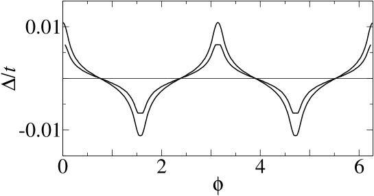
FIG. 3.: Gap function for $n=0.88$ (larger amplitude) and $n=0.9$ (smaller amplitude) as a function of the angle with respect to the $k_{x}$-axis.

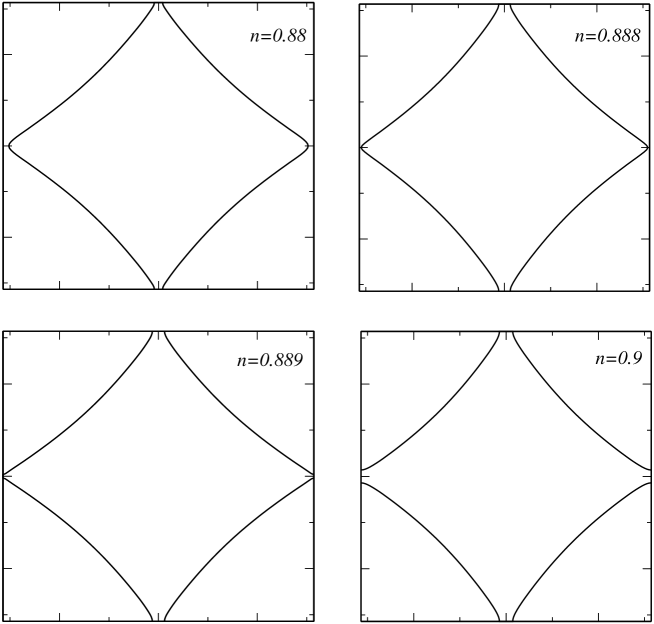
FIG. 4.: Fermi surfaces of the interacting system for different densities $n$.

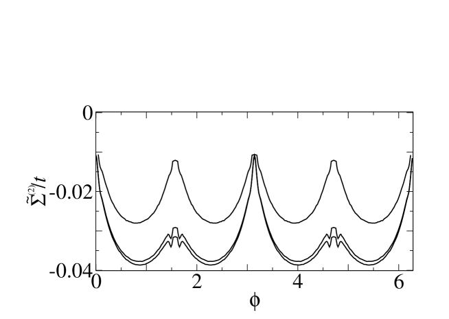
FIG. 5.: Second-order counterterms $\tilde{\Sigma}^{(2)}(0,\tilde{\bf k}_{F})$ as a function of the angle with respect to the $k_{x}$-axis, for the densities $n=0.888,0.889,0.9$ (from bottom to top).

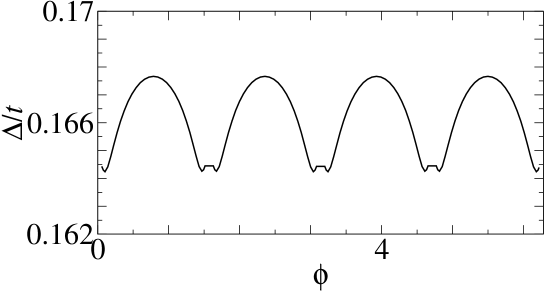
FIG. 6.: Gap function for $n=0.9$ as a function of the angle with respect to the $k_{x}$-axis for the attractive ($U=-2t$) Hubbard model.

REFERENCES

- [1] G. Baym and L.P. Kadanoff, Phys. Rev. 124, 287 (1961); G. Baym, Phys. Rev. 127, 1391 (1962).
- [2] P. Nozières, Theory of Interacting Fermi Systems (Benjamin, New York, 1964).
- [3] J. Feldman, J. Magnen, V. Rivasseau, and E. Trubowitz, in The State of Matter, edited by M. Aizenmann and H. Araki, Advanced Series in Mathematical Physics Vol. 20 (World Scientific 1994).
- [4] J. Feldman, H. Knörrer, M. Salmhofer, and E. Trubowitz, J. Stat. Phys. 94, 113 (1999).
- [5] See, for example, D.J. Scalapino, Phys. Rep. 250, 329 (1995); D.J. Scalapino and S.R. White, Found. Phys. 31, 27 (2001).
- [6] D. Zanchi and H.J. Schulz, Phys. Rev. B 61, 13609 (2000); C.J. Halboth and W. Metzner, Phys. Rev. B 61, 7364 (2000); C. Honerkamp, M. Salmhofer, N. Furukawa, and T.M. Rice, Phys. Rev. B 63, 035109 (2001).
- [7] C.J. Halboth and W. Metzner, Phys. Rev. Lett. 85, 5162 (2000).
- [8] H. Yamase and H. Kohno, J. Phys. Soc. Jpn. 69, 332 (2000); 69, 2151 (2000).
- [9] I. Grote, E. Körding, and F. Wegner, J. Low Temp. Phys. 126, 1385 (2002); V. Hankevych, I. Grote and F. Wegner, condmat/0205213; V. Hankevych and F. Wegner, cond-mat/0207612.
- [10] See, for example, J.W. Negele and H. Orland, Quantum Many-Particle Systems (Addison-Wesley, Reading, MA, 1987).
- [11] J. Feldman, M. Salmhofer, and E. Trubowitz, J. Stat. Phys. 84, 1209 (1996); Commun. Pure Appl. Math. 51, 1133 (1998); Commun. Pure Appl. Math. 52, 273 (1999).
- [12] A. Georges and J.S. Yedidia, Phys. Rev. B 43, 3475 (1991).
- [13] See, for example, The Hubbard Model, edited by A. Montorsi (World Scientific, Singapore, 1992).
- [14] Also small numerical errors can be sufficient to start the symmetry breaking in the iteration procedure.
- [15] S.A. Kivelson, E. Fradkin, and V.J. Emery, Nature 393, 550 (1998).
- [16] V. Oganesyan, S.A. Kivelson, and E. Fradkin, Phys. Rev. B 64, 195109 (2001).
- [17] M. Vojta, Y. Zhang, and S. Sachdev, Phys. Rev. Lett. 85, 4940 (2000); Int. J. Mod. Phys. B 14, 3719 (2000).
- [18] For a review of the attractive Hubbard model (and extensions), see R. Micnas, J. Ranninger, and S. Robaszkiewicz, Rev. Mod. Phys. 62, 113 (1990).
- [19] P.G.J. van Dongen, Phys. Rev. Lett. 67, 757 (1991).