Probing Vortex Unbinding via Dipole Fluctuations

Abstract

We develop a numerical method for detecting a vortex unbinding transition in a two-dimensional system by measuring large scale fluctuations in the total vortex dipole moment ${\vec{P}}$ of the system. These are characterized by a quantity $\cal F$ which measures the number of configurations in a simulation for which the either $P_{x}$ or $P_{y}$ is half the system size. It is shown that $\cal F$ tends to a non-vanishing constant for large system sizes in the unbound phase, and vanishes in the bound phase. The method is applied to the $XY$ model both in the absence and presence of a magnetic field. In the latter case, the system size dependence of $\cal F$ suggests that there exist three distinct phases, one unbound vortex phase, a logarithmically bound phase, and a linearly bound phase.

PACS numbers: 05.10.-a, 64.60.-i, 75.10.Hk

Introduction – Topological defects play a crucial role in two dimensional classical systems[1] and in 1+1 dimensional quantum systems[2]. The paradigm of these is the $XY$ model, which is known to undergo a vortex-unbinding transition in the Kosterlitz-Thouless (KT) universality class [3]. Highly analogous transitions occur for vortices in superfluids and thin-film superconductors, as well as for dislocations and disclinations in two dimensional crystals. Wordline dislocations in one dimensional quantum systems are important for describing tunneling [4], and the question of whether these are bound or unbound is closely related to whether the system is metallic or insulating.

The KT phenomenology has been highly successful in describing defect unbinding in a variety of situations. For the $XY$ model, fitting to the expected finite-size scaling of the helicity modulus in simulations yields an estimate of $T_{KT}=0.892$ [5]. However, the concepts of vortices and defect unbinding are more general than the systems in which a KT transition takes place. In some situations a symmetry-breaking field, for example, a magnetic field tending to align the spins in the $XY$ model, may be present [6]. A recent renormalization group (RG) study [7] has suggested that vortex unbinding does occur in such systems, although the transition is considerably altered from the KT behavior. It is thus important to develop criteria by which one may determine whether a given system is in a bound or unbound vortex state which are independent of precise matching to the KT theory. In this article, we present a method by which this may be accomplished, which focuses on a measure $\cal F$ of extreme fluctuations in the system vortex dipole moment. Using a Langevin dynamics simulation of the $XY$ model, we show that the method locates $T_{KT}$ with reasonable accuracy. We then include a magnetic field in the Hamiltonian, and show that there are both bound and unbound vortex phases. The bound phase has two distinct behaviors: for smaller fields, $\cal F$ vanishes as a power of the system size $L$; for larger fields, $\cal F$ vanishes exponentially with $L$. The two behaviors are consistent with the results of the RG analysis [7], which predicted both a logarithmically bound vortex phase and a linearly confined one, in addition to the unbound (deconfined) vortex phase.

Characterizing Vortex Dipole Fluctuations – A total vortex dipole moment may be defined for configurations of any system containing vortices with well-defined locations. For concreteness, we will work with the $XY$ model (planar spins of fixed length) on a square lattice. Let $\Delta\theta_{ij}$ denote the angular difference between nearest neighbor spins $ij$, which we reduce to the interval $-\pi<\Delta\theta_{ij}\leq\pi$ by adding or subtracting $2\pi$ if necessary. The vorticity $q_{i}$ around an elementary plaquette $P$ is then $q_{i}=(1/2\pi)\sum_{P}\Delta\theta_{ij}$, which takes on the values $-1,$ $0$, $1$[8]. For any configuration of the $XY$ system this rule assigns vortex charges to the sites ${\vec{R}}_{i}$ of the dual lattice. The corresponding dipole moment could be defined by

$${\vec{P}}=\sum q_{i}{\vec{R}}_{i}.$$ (1)

However, there is a problem associated with the use of periodic boundary conditions: for a $L\times L$ system one may add $(n^{x}_{i}L,n^{y}_{i}L)$ to ${\vec{R}}_{i}$ (with $n^{x}_{i},~{}n^{y}_{i}$ integers) and retain a perfectly sensible definition of ${\vec{P}}$. For a given configuration, we can use this to reduce $\vec{P}$ so that its components are restricted to the interval $-L/2\leq P_{x,y}\leq L/2$; or we can extend its definition by adding factors of $L$ so that $\vec{P}$ remains a continuous function as a vortex crosses a periodicity boundary. We will refer to these alternate definitions of the dipole moment as ${\vec{P}}_{red}$ and ${\vec{P}}_{ext}$, respectively. Note that $P^{x,y}_{red}$ will jump discontinuously by $L$ whenever a vortex crosses a boundary.

The bound vortex phase has the property that the dipole moment remains finite, since the pairs do not separate; in the unbound phase, the diffusion of vortices implies a diffusion of the dipole moment, so that its magnitude can become arbitrarily large. In a finite system, this presumably translates into the statement that the diffusion of ${\vec{P}}_{ext}$ becomes very small below the unbinding temperature.

A feature of vortex unbinding transitions is that the transition occurs via rare but extreme fluctuations [9]. One way to characterize such fluctuations is to look for system configurations with extreme values of ${\vec{P}}_{red}$. Loosely speaking, if we wish to characterize a configuration in terms of an effective single vortex-antivortex pair, when $P_{x}$ or $P_{y}$ is $L/2$, the pair is at its maximum separation. If such extreme configurations persist as $L\rightarrow\infty$, the system is then in an unbound phase. By contrast, we expect the number of such configurations to vanish in the large size limit when the system is in a bound phase.

This expectation may be more carefully justified by considering effective theories of vortices in their bound and unbound phases. An unbound vortex system behaves as a two-dimensional metal in which the discreteness of the underlying vortex charges may be neglected. An effective Hamiltonian takes the form [10]

$$H_{unb}^{eff}={K\over 2}\int d^{2}xd^{2}x^{\prime}\rho({\vec{x}})G(|{\vec{x}}-{\vec{x}^{\prime}}|)\rho({\vec{x}^{\prime}})+{{\mu}\over 2}\int d^{2}x\rho^{2}({\vec{x}}),$$ (2)

where $G(r)\sim-(2\pi)^{-1}\log(r/a)+$const, with $a$ a microscopic length of order the lattice constant of the system, and $\mu$ is an effective chemical potential, essentially the core energy of the vortices. For this continuum system, we can adopt a definition of the ($x$-component of the) dipole moment which incorporates the periodic boundary condition,

$$P^{x}_{eff} ={L\over{2\pi}}\int d^{2}x\rho({\vec{x}})\sin\bigl{[}{{2\pi x}\over L}\bigl{]}$$ (3)

$$={L\over{2\pi}}Im\{\rho(k_{x}=2\pi/L,k_{y}=0)\}.$$ (4)

The fraction ${\cal F}$ of configurations with $P^{x}_{eff}=L/2$ is thus given by the probability of finding $Im\{\rho(k_{x}=2\pi/L,k_{y}=0)=\pi$. This is easily evaluated by re-expressing $H_{unb}^{eff}$ in terms of a wavevector sum instead of a real space integral. Noting that the Fourier transform of $G(r)$ for small wavevectors is $G(k)\sim 1/k^{2}$, one obtains

$${\cal F}\propto e^{-{1\over{L^{2}T}}[{1\over 2}K\bigl{(}{L\over{2\pi}}\bigr{)}^{2}+\mu]}\approx e^{-K/8\pi^{2}T}$$ (5)

for the probability of obtaining an extreme dipole fluctuation in the large size limit. Notice the ${\cal F}$ does not vanish as $L\rightarrow\infty$, supporting our argument above that large dipole fluctuations survive in the unbound vortex state.

To analyze the bound vortex state, we focus on the two dimensional Coulomb particle Hamiltonian

$$H_{CG}={K\over 2}\int d^{2}xd^{2}x^{\prime}m({\vec{x}})G(|{\vec{x}}-{\vec{x}^{\prime}}|)m({\vec{x}^{\prime}}),$$ (6)

where $m({\vec{x}})$ is an integer degree of freedom, and the partition function involves a sum over all complexions of $m$ satisfying $\int d^{2}xm({\vec{x}})=0$. The probability of an extreme fluctuation in the system dipole moment may be expressed as

$${\cal F}\propto\sum_{\{m\}}e^{-H_{CG}[m]/T}\delta[Im~{}m({\vec{k}}_{d})-\pi]$$ (7)

$$=\int_{-\infty}^{\infty}d\lambda e^{-i\lambda\pi}\sum_{\{m\}}e^{-H_{CG}[m]/T}e^{i\lambda Im~{}m({\vec{k}}_{d})},$$ (8)

where we have adopted the same definition of $P^{x}_{eff}$ as in Eq.4, with $\rho({\vec{x}})$ replaced by $m({\vec{x}})$, and ${\vec{k}}_{d}\equiv(2\pi/L,0)$. In the bound state the integer nature of $m({\vec{x}})$ may not be ignored; however, we can make progress by adopting the dual description of the partition function [6]. This involves employing the Poisson resummation formula to rewrite Eq. 8 as

$${\cal F}\propto\int_{-\infty}^{\infty}d\lambda e^{-i\lambda\pi}\int{\cal D}\phi\sum_{\{n\}}e^{-H_{CG}[\phi]/T}e^{i\lambda Im~{}\phi({\vec{k}}_{d})}e^{-2\pi i\sum_{\vec{x}}\phi({\vec{x}})n({\vec{x}})}.$$ (10)

The integration over the continuous field $\phi$ may be carried through, with the result

$${\cal F}\propto\int_{-\infty}^{\infty}d\lambda e^{-i\lambda\pi}\sum_{\{n\}}e^{-{T\over{2K}}\sum_{\vec{k}}|2\pi n({\vec{k}})-\lambda Im~{}n({\vec{k}}_{d})~{}\delta_{{\vec{k}},{\vec{k}}_{d}}|^{2}/G(k)}.$$ (11)

A bound vortex fixed point is generated by replacing $K$ with a renormalized value, and exchanging the sum over integers $n$ in Eq. 11 with a functional integral over continuous fields [11]. The resulting model represents the rough phase of a solid-on-solid model. Once the integer sum has been replaced by an integral, the $\lambda Im~{}n({\vec{k}}_{d})$ term in the integrand may be shifted away and the functional integral in fact has no dependence on $\lambda$. It then immediately follows that ${\cal F}=0$ for the bound vortex phase.

These considerations lead us to expect that one should observe large vortex dipole fluctuations in the unbound phase, but not in the bound one. We now demonstrate this is indeed the case using a Langevin dynamics simulation.

Simulation – Our simulations focus on the $XY$ model for which we assign dynamics to the spins and coupling to a heat bath to generate a distribution of configurations. The equations of motion for our system are taken to be

$$\Gamma{{d^{2}\theta({\vec{x}})}\over{dt^{2}}}={{\delta H_{XY}}\over{\delta\theta({\vec{x}})}}+\zeta({\vec{x}})-\eta{{d\theta({\vec{x}})}\over{dt}}.$$ (12)

$\Gamma$ is an effective moment of inertia for the $XY$ spins, which for simplicity we set to 1 in the simulations, $\zeta$ is a random torque which models coupling to a heat bath, and $\eta$ is a viscosity. To satisfy the fluctuation-dissipation theorem, the random torques are drawn from a distribution satisfying $<\zeta(\vec{r},t)\zeta(\vec{r}^{\prime},t^{\prime})>=2\eta T\delta_{\vec{r},\vec{r}^{\prime}}\delta(t-t^{\prime})$ with $T$ the temperature of the system. Finally, our $XY$ Hamiltonian is

$$H_{XY}=-K\sum_{<{\vec{x}},{\vec{x}}^{\prime}>}cos[\theta({\vec{x}})-\theta({\vec{x}}^{\prime})]-h\sum_{\vec{x}}cos\theta({\vec{x}})$$ (13)

where we take the angles $\theta({\vec{x}})$ to reside on an $L\times L$ square lattice. To perform the simulation, we have discretized the time derivative in Eq. 12 and used a standard random number generator [12] to generate a realization of $\zeta(\vec{r},t)$ at each time step. A typical run consists of $10^{6}$ Langevin sweeps for equilibration, followed by $9\times 10^{6}$ measurement steps. In accumulating the data, we repeated runs for each set of parameters with $\sim 10$ different seeds, allowing us to estimate our statistical errors. Simulations were performed for system sizes as large as $L=199$, although most of the simulations were in the range $19\leq L\leq 59$.

Our measurement consists of counting the number of times a component of the system dipole moment ${\vec{P}}_{ext}$ passes through $(n+{1\over 2})L$ for $n$ any integer. We then plot the number of such events divided by the total simulation time, yielding a measure of the fraction of configurations $\cal F$ for which the system has attained its maximal value. One advantage of the Langevin dynamics approach is that the vortex dipole moment ${\vec{P}}_{ext}$ changes by several steps with each Langevin sweep, but these steps are always much smaller than $L$ except for very small values of $L$. This allows us to detect when ${\vec{P}}_{ext}$ has passed through $(n+{1\over 2})L$ even if in the immediate time step before and the step after ${\vec{P}}_{ext}$ was not measured to be precisely at this value. A larger number of events can then be accumulated than one might in a Monte Carlo simulation employing a cluster algorithm, since the configurations generated in the latter are not related in any simple way, forcing one to count only configurations for which ${\vec{P}}_{ext}$ is precisely $(n+{1\over 2})L$. Note that we count passages in both directions; this tells us how often ${\vec{P}}_{red}$ visits its extremal value.

As a check on the method, we first present results of simulations in the absence of the symmetry-breaking field, for which vortices unbind in a Kosterlitz-Thouless transition. Fig. 1 illustrates these for $L=59$, $h=0$ and $K=1$. One can see $\cal F$ decreases sharply as the temperature approaches $T\approx 0.9$ from above, so that $\cal F$ appears to be vanishing quite close to the accepted value of $T^{XY}_{KT}=0.892$. The differing behavior of $\cal F$ above and below the transition can be further confirmed by examining its size dependence: for $T$ below the transition temperature, $\cal F$ decreases with system size, apparently approaching zero as $L\rightarrow\infty$, whereas for higher values of $T$, $\cal F$ increases, approaching a constant value from below. These differing size dependences strongly support the idea that $\cal F$ distinguishes the bound and unbound phases.

We now turn to the case $h>0$, for which we show some typical results in Fig. 2. The behavior of $\cal F$ as a function of system size takes three differing forms, depending on the values of $h$ and $T$. At high temperature and low fields, $\cal F$ clearly approaches a non-vanishing value in the large system size limit (e.g., $h=0.18$ curve in Fig. 2). Unlike the $h=0$ case the asymptotic value of $\cal F$ is approached from above, indicating the that symmetry breaking field has had some effect, although for small enough $h$ the vortices remain unbound. At intermediate values of $h$, we find $\cal F$ decreasing as a power law in $1/L$ ($h=0.3$ curve), indicating a bound vortex phase behaving as one would expect for logarithmically interacting vortices. Finally, at the largest values of $h$ ($h=0.5$ curve), $\cal F$ decreases exponentially with $L$, as might be expected for vortices interacting with a linear binding potential.

Our results indicate that in the presence of a magnetic field, there exists an unbound vortex state and two different bound vortex states in the $XY$ model. This behavior is precisely what was predicted in the $RG$ analysis of Ref. [7]. At low temperatures, vortex-antivortex pairs are connected by a string of overturned spins, leading to linear confinement. As temperature is increased, fluctuations can lead to a roughening of the strings binding the vortices, driving the effective string tension to zero. The vortex-antivortex pairs nevertheless retain a logarithmic attraction and remain bound as the system passes through the transition. At still higher temperatures, a second transition occurs in which the vortices do ultimately unbind. A remarkable feature of these transitions is that they are extremely continuous[7], so that no singularity is expected in the free energy as the transitions occur. Measurements of the specific heat and magnetization in our simulations show no indications of any such singularities. Thus, one is forced to probe the vortices directly in order to detect their unbinding, as we have done by probing the system vortex dipole moment. It is interesting to note that, in the absence of singularities in the free-energy, it is unclear whether vortex unbinding should be thought of as a true thermodynamic phase transition. To our knowledge, this is the first example of a defect-unbinding transition that does not have the full character of a phase transition.

In summary, we have developed a method of detecting vortex unbinding in two-dimensional systems by tracking extreme fluctuations in the vortex dipole moment of the system. For a system of size linear $L$, the fraction of configurations $\cal F$ having a dipole moment component $P_{x}$ or $P_{y}$ equal to its largest value consistent with periodic boundary conditions ($L/2$) approaches a constant for large sizes when vortices are unbound, and vanishes when vortices are bound. We have demonstrated this for the Kosterlitz-Thouless transition in $XY$ model, for which $\cal F$ can locate the transition temperature with reasonable accuracy. In the presence of a magnetic field tending to orient the spins, we have found that there is an unbound vortex state and two possible bound vortex states, one consistent with logarithmic binding of the vortices, the other with linear confinement. The method presented here is easily generalizable, and should be applicable to systems with other topological, point-like defects.

Acknowledgments – The authors are indebted to the Center for Computational Sciences at the University of Kentucky for providing computer time. Helpful discussions with Dr. Donald Priour are gratefully acknowledged. This work was supported by NSF Grant No. DMR-01-08451.

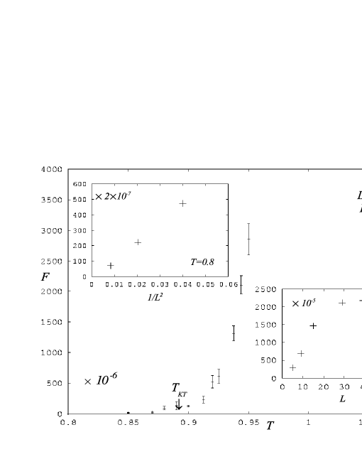
FIG. 1.: $F$ vs. temperature for $XY$ system with $h=0$, $L=59$. $F$ drops sharply in vicinity of the known Kosterlitz-Thouless temperature. Left inset: $F$ vs. $1/L^{2}$ for $T=0.8$, demonstrating $F$ vanishes in the bound vortex state. Right inset: $F$ vs. $L$ for $T=1.2$, demonstrating $F$ approaches a non-zero constant in the unbound vortex state.

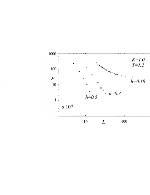
FIG. 2.: $F$ vs. system size for $XY$ system for $h=0.18,~{}0.30,~{}0.50$ for fixed temperature $T=1.2$ $F$ approaches a constant for large system sizes for smallest field, vanishes as a power law for intermediate field (straight line on log-log plot), and vanishes exponentially for largest field (downward curvature on log-log plot). The three different behaviors indicate one unbound vortex phase, logarithmically bound phase, and a linearly confined phase.

REFERENCES

- [1] D.R. Nelson, Defects and Geometry in Condensed Matter Physics, (Cambridge University Press, New York, 2002).
- [2] A.O. Gogolin, A.A. Nersesyan, and A.M. Tsvelik, Bosonization and Strongly Correlated Systems,” (Cambridge University Press, New York, 1998).
- [3] J.M. Kosterlitz and D. Thouless, J. Phys. C: Solid State Phys. 6, 1181 (1973); J.M. Kosterlitz, Phys. C: Solid State Phys. 7, 1046 (1974).
- [4] E. Kolomeisky and J.P. Straley, Rev. Mod. Phys. 68, 175 (1996).
- [5] P. Olsson, Phys. Rev. B 52, 4526 (1995).
- [6] J.V. José, L.P. Kadanoff, S. Kirkpatrick, and D.R. Nelson, Phys. Rev. B 16, 1217 (1977).
- [7] H.A. Fertig, Phys. Rev. Lett. 89, 035703 (2002).
- [8] The sum of the does not necessarily vanish. This is a consequence of having constrained these to the finite interval.
- [9] N.D. Antunes, L.M.A. Bettencourt, and M. Kunz, cond-mat/0201149.
- [10] G. Foltin, cond-mat/0101060.
- [11] P.M. Chaikin and T.C. Lubensky, Principles of Condensed Matter Physics, (Cambridge University Press, New York, 1995).
- [12] W.H. Press, S.A. Teukolsky, W.T. Vetterling, and B.P. Flannery, Numerical Recipes, Second Ed., (Cambridge University Press, New York, 1996). We used the program ran1.f they describe.