Scattering matrix ensemble for time-dependent transport through a chaotic quantum dot

Abstract

Random matrix theory can be used to describe the transport properties of a chaotic quantum dot coupled to leads. In such a description, two approaches have been taken in the literature, considering either the Hamiltonian of the dot or its scattering matrix as the fundamental random quantity of the theory. In this paper, we calculate the first four moments of the distribution of the scattering matrix of a chaotic quantum dot with a time-dependent potential, thus establishing the foundations of a “random scattering matrix approach” for time-dependent scattering. We consider the limit that the number of channels $N$ coupling the quantum dot the reservoirs is large. In that limit, the scattering matrix distribution is almost Gaussian, with small non-Gaussian corrections. Our results reproduce and unify results for conductance and pumped current previously obtained in the Hamiltonian approach. We also discuss an application to current noise.

1 Introduction

From a statistical point of view, energy levels and wavefunctions in semiconductor quantum dots and metal grains, or eigenfrequencies and eigenmodes of microwave cavities, share a remarkable universality. With proper normalization, correlation functions of energy levels or wavefunctions for an ensemble of macroscopically equivalent, but microscopically distinct samples depend on the fundamental symmetries of the sample only; they do not depend on sample shape or volume, or on the impurity concentration. The same universality appears for correlators of eigenvalues and eigenfunctions of large matrices with randomly chosen elements [1, 2, 3]. Originally, such “random matrices” were introduced by Wigner and Dyson to describe the universal features of spectral correlations in heavy nuclei [4, 5]. Theoretical predictions from random matrix theory have been verified in experiments on semiconductor quantum dots and chaotic microwave cavities, and with the help of numerical simulations [6, 7, 8, 9]; for the case of a disordered quantum dot, the validity of random matrix theory has been proven by field-theoretic methods [10].

Open samples, such as semiconductor quantum dots coupled to source and drain reservoirs by means of ballistic point contacts or microwave cavities coupled to ideal waveguides, do not have well-resolved energy levels or wavefunctions. They are characterized by means of a continuous density of states and by their transport properties, such as conductance or shot noise power. Within random-matrix theory, two approaches have been taken to describe open samples [11]. In both approaches, transport properties are described in terms of the sample’s scattering matrix ${\cal S}$. The first approach is the “random Hamiltonian approach”. In this approach, the scattering matrix is expressed in terms of a random Hermitean matrix $H$, which represents the Hamiltonian of the closed sample. Averages or fluctuations of transport properties are then calculated in terms of the known statistical distribution of the random matrix $H$ [12, 13]. In the second approach, the “random scattering matrix approach”, the scattering matrix ${\cal S}$ itself is considered the fundamental random quantity. It is taken from Dyson’s “circular ensemble” of uniformly distributed random unitary matrices [14, 15, 16, 17, 18], or a generalization known as the “Poisson kernel” [2, 19, 20]. Both approaches were shown to be equivalent [13, 20]. Hence, in the end, which method to use is a matter of taste.

Recently, there has been interest in transport through chaotic quantum dots with a time-dependent Hamiltonian. Switkes et al. fabricated a “quantum electron pump” consisting of a chaotic quantum dot of which the shape could be changed by two independent parameters [21]. Periodic variation of the shape then causes current flow through the quantum dot, hence the name “electron pump”. Motivated by theoretical predictions of Vavilov and Aleiner [22, 23], Huibers et al. looked at the effect of microwave radiation on the quantum interference corrections to the conductance of a quantum dot [24]. The presence of a time-dependent potential will cause the ratio of universal conductance fluctuations with and without time-reversal symmetry to be less than two if the typical frequency of the fluctuations is of the order of the electron escape rate from the quantum dot [23, 25, 26, 27]. (By the Dyson-Mehta theorem [28], the ratio is two in the absence of a time-dependent perturbation [11].)

A scattering matrix formalism to describe time-dependent transport was developed by Büttiker and coworkers [29, 30, 31, 32, 33]. The scattering matrix formalism for time-dependent scattering is more complicated than the formalism for time-independent scattering, since energy is no longer conserved upon scattering from a cavity or quantum dot with a time-dependent potential. In the adiabatic limit, when the frequency $\omega$ of the time-dependent variations is small compared to the escape rate from the quantum dot, the theory can be formulated in terms of the scattering matrix ${\cal S}$ and its derivative to energy [32]. However, a theory that describes arbitrary frequencies $\omega$ must be formulated in terms of a scattering matrix ${\cal S}(\varepsilon,\varepsilon^{\prime})$ that depends on two energy arguments, or, equivalently, a matrix ${\cal S}(t,t^{\prime})$ depending on two time arguments [22].

Random matrix theory can be used to describe the statistics of time-dependent transport if the time dependence is slow on the scale of the time $\tau_{\rm erg}$ needed for ergodic exploration of the quantum dot. In several recent papers [22, 23, 25, 26, 27, 34, 35], the calculation of time-dependent transport properties for an ensemble of chaotic quantum dots was done using a variation of the “random Hamiltonian approach”: the time-dependent scattering matrix ${\cal S}(t,t^{\prime})$ is first expressed in terms of a time-dependent Hermitean matrix $H(t)$, which is the sum of a time-independent random matrix and a time-dependent matrix which does not need to be random; the ensemble average is then calculated by integrating $H$ over the appropriate distribution of random matrices. It is the purpose of this paper to develop a “random scattering matrix approach” for time-dependent scattering, using the distribution of the scattering matrix ${\cal S}(t,t^{\prime})$, not the Hamiltonian $H(t)$, as the starting point for further calculations.

For time-independent scattering, the distribution of the elements of the scattering matrix is given by the circular ensembles from random matrix theory (or, for a quantum dot with non-ideal leads, by the Poisson kernel). In the limit that the dimension $N$ of the scattering matrix becomes large, the scattering matrix distribution can be well approximated by a Gaussian, whereas non-Gaussian correlations can be accounted for in a systematic expansion in $1/N$ [36]. For the calculation of transport properties (conductance, shot noise power), the Gaussian approximation is usually sufficient; knowledge of the underlying “full” scattering matrix distribution is not required. Here, we take a similar approach for time-dependent transport. We show that, for large $N$, elements of the scattering matrix ${\cal S}(t,t^{\prime})$ are almost Gaussian random numbers, for which non-Gaussian correlations can be taken into account by means of a systematic expansion in $1/N$. We calculate the second moment of the distribution and the leading non-Gaussian correction.

This paper is organized as follows: In section 2 we review the scattering matrix approach for time-independent scattering. The case of time-dependent scattering is considered in section 3. Applications are discussed in section 4. Details of the calculation and an extension to the case of quantum dots with nonideal contacts can be found in the appendices. The second moment of the scattering matrix distribution calculated here was used in reference [37] to compute the shot noise power of a quantum electron pump.

2 Time-independent scattering

We first summarize important facts about the distribution of the scattering matrix ${\cal S}$ for time-independent scattering.

For large matrix size $N$, the scattering matrix elements ${\cal S}_{ij}$ have a Gaussian distribution with small non-Gaussian correlations. Mathematically, this is a consequence of the fact that ${\cal S}$ is distributed according to the circular ensemble from random matrix theory or, for a quantum dot with non-ideal leads, the Poisson kernel [36]. In a semiclassical picture, the Gaussian distribution of the scattering matrix elements follows from the central limit theorem, when ${\cal S}_{ij}$ is written as a sum over many paths, where the contribution of each path contains a random phase factor [14, 15, 16, 38, 39]. The small non-Gaussian corrections follow because the full scattering matrix satisfies the constraint of unitarity, which is not imposed in the semiclassical formulation.

The Gaussian part of the distribution is characterized by the first two moments. In the main text, we focus on the case of a quantum dot coupled to the outside world via ideal leads. In this case, the first moment vanishes,

$$\langle{\cal S}_{ij}\rangle=0.$$ (1)

The case of nonideal leads, for which $\langle{\cal S}_{ij}\rangle\neq 0$, is discussed in appendix A. The second moment of the scattering matrix distribution depends on the presence or absence of time-reversal symmetry (TRS),

$$W_{1}^{ij;kl}=\langle{\cal S}_{ij}{\cal S}_{kl}^{*}\rangle = {1\over N}\times\left\{\begin{array}[]{ll}(\delta_{ik}\delta_{jl}+\delta_{il}\delta_{jk})&\mbox{with TRS},\\ \delta_{ik}\delta_{jl}&\mbox{without TRS},\end{array}\right.$$ (4)

up to corrections of relative order $1/N$ in the presence of time-reversal symmetry. All averages involving unequal powers of ${\cal S}$ and ${\cal S}^{*}$ vanish. Equation (4) is for spinless particles or for electrons with spin in the absence of spin-orbit coupling. (In the latter case, the scattering matrix has dimension $2N$ and is of the form ${\cal S}\otimes{\bf 1}_{2}$, where ${\bf 1}_{2}$ is the $2\times 2$ unit matrix in spin space and the $N\times N$ matrix ${\cal S}$ describes scattering between orbital scattering channels.) We do not consider the case of broken spin-rotation symmetry, when ${\cal S}$ is a random matrix of quaternions [1].

Non-Gaussian correlations of scattering matrices are of relative order $1/N$ or less. The leading non-Gaussian correlations are described by the cumulant [42, 43, 36]

$$W_{2}^{i_{1}j_{1},i_{2}j_{2};k_{1}l_{1},k_{2}l_{2}}=\langle{\cal S}_{i_{1}j_{1}}{\cal S}_{i_{2}j_{2}}{\cal S}_{k_{1}l_{1}}^{*}{\cal S}_{k_{2}l_{2}}^{*}\rangle-\langle{\cal S}_{i_{1}j_{1}}{\cal S}_{k_{1}l_{1}}^{*}\rangle\langle{\cal S}_{i_{2}j_{2}}{\cal S}_{k_{2}l_{2}}^{*}\rangle$$

$$\mbox{}-\langle{\cal S}_{i_{1}j_{1}}{\cal S}_{k_{2}l_{2}}^{*}\rangle\langle{\cal S}_{i_{2}j_{2}}{\cal S}_{k_{1}l_{1}}^{*}\rangle.$$ (5)

In the absence of time-reversal symmetry and for $N\gg 1$, the cumulant $W_{2}$ is given by

$$W_{2} = -{1\over N^{3}}\left(\delta_{i_{1}k_{1}}\delta_{j_{1}l_{2}}\delta_{i_{2}k_{2}}\delta_{j_{2}l_{1}}+\delta_{i_{1}k_{2}}\delta_{j_{1}l_{1}}\delta_{i_{2}k_{1}}\delta_{j_{2}l_{2}}\right),$$ (6)

In the presence of time-reversal symmetry, $W_{2}$ is found by the addition of 14 more terms to equation (6), corresponding to the permutations $i_{2}\leftrightarrow j_{2}$, $k_{1}\leftrightarrow l_{1}$, and $k_{2}\leftrightarrow l_{2}$,

$$W_{2}=-{1\over N^{3}}\left(\delta_{i_{1}k_{1}}\delta_{j_{1}l_{2}}\delta_{i_{2}k_{2}}\delta_{j_{2}l_{1}}+\delta_{i_{1}k_{2}}\delta_{j_{1}l_{1}}\delta_{i_{2}k_{1}}\delta_{j_{2}l_{2}}+\delta_{i_{1}k_{1}}\delta_{j_{1}l_{2}}\delta_{j_{2}k_{2}}\delta_{i_{2}l_{1}}+\delta_{i_{1}k_{2}}\delta_{j_{1}l_{1}}\delta_{j_{2}k_{1}}\delta_{i_{2}l_{2}}\right.$$

$$\left.\mbox{}+\delta_{i_{1}l_{1}}\delta_{j_{1}l_{2}}\delta_{i_{2}k_{2}}\delta_{j_{2}k_{1}}+\delta_{i_{1}k_{2}}\delta_{j_{1}k_{1}}\delta_{i_{2}l_{1}}\delta_{j_{2}l_{2}}+\delta_{i_{1}l_{1}}\delta_{j_{1}l_{2}}\delta_{j_{2}k_{2}}\delta_{i_{2}k_{1}}\right.$$

$$\left.\mbox{}+\delta_{i_{1}k_{2}}\delta_{j_{1}k_{1}}\delta_{j_{2}l_{1}}\delta_{i_{2}l_{2}}+\delta_{i_{1}k_{1}}\delta_{j_{1}k_{2}}\delta_{i_{2}l_{2}}\delta_{j_{2}l_{1}}+\delta_{i_{1}l_{2}}\delta_{j_{1}l_{1}}\delta_{i_{2}k_{1}}\delta_{j_{2}k_{2}}\right.$$

$$\left.\mbox{}+\delta_{i_{1}k_{1}}\delta_{j_{1}k_{2}}\delta_{j_{2}l_{2}}\delta_{i_{2}l_{1}}+\delta_{i_{1}l_{2}}\delta_{j_{1}l_{1}}\delta_{j_{2}k_{1}}\delta_{i_{2}k_{2}}+\delta_{i_{1}l_{1}}\delta_{j_{1}k_{2}}\delta_{i_{2}l_{2}}\delta_{j_{2}k_{1}}\right.$$

$$\left.\mbox{}+\delta_{i_{1}l_{2}}\delta_{j_{1}k_{1}}\delta_{i_{2}l_{1}}\delta_{j_{2}k_{2}}+\delta_{i_{1}l_{1}}\delta_{j_{1}k_{2}}\delta_{j_{2}l_{2}}\delta_{i_{2}k_{1}}+\delta_{i_{1}l_{2}}\delta_{j_{1}k_{1}}\delta_{j_{2}l_{1}}\delta_{i_{2}k_{2}}\right).$$ (7)

We refer to reference [36] for higher-order cumulants and finite-$N$ corrections to $W_{1}$ and $W_{2}$.

Although equations (4) and (5) do not specify the full scattering matrix distribution — for that one would need to know all cumulants —, they are sufficient to calculate the average and variance of most transport properties. As an example, we consider a quantum dot connected to source and drain reservoirs by means of two ballistic point contacts with $N_{1}$ and $N_{2}$ propagating channels per spin direction at the Fermi level, with $N=N_{1}+N_{2}$. The zero-temperature conductance is given by the Landauer formula, which we write as [40]

$$G={2e^{2}\over h}\left({N_{1}N_{2}\over N}-\tr{\cal S}\Lambda{\cal S}^{\dagger}\Lambda\right),$$ (8)

where $\cal S$ is the $N\times N$ scattering matrix and $\Lambda$ is an $N\times N$ diagonal matrix with

$$\Lambda_{ij}={\delta_{ij}\over N}\times\left\{\begin{array}[]{ll}N_{2}&\mbox{if $1\leq i\leq N_{1}$},\\ -N_{1}&\mbox{if $N_{1}<i\leq N$}.\end{array}\right.$$ (9)

For large $N$, the second term in equation (8) is a small and fluctuating quantum correction to the classical conductance of the quantum dot. Using equations (4) and (6), the average and variance of the conductance for $N\gg 1$ then follow as

$$\langle G\rangle = {2e^{2}\over h}\left({N_{1}N_{2}\over N}-\delta_{\beta,1}{N_{1}N_{2}\over N^{2}}\right)\ \$$ (10)

$$\mbox{var}\,G = {4e^{4}\over h^{2}}\left({N_{1}^{2}N_{2}^{2}\over N^{4}}\right)(1+\delta_{\beta,1}),$$ (11)

where the symmetry parameter $\beta=1$ or $2$ with or without time-reversal symmetry, respectively.

In the derivation of equations (10) and (11) it is important that the matrix $\Lambda$ is traceless. This ensures that the non-Gaussian cumulant (6) does not contribute to $\mbox{var}\,G$, despite the fact that calculation of $\mbox{var}\,G$ involves an average over a product of four scattering matrices. Similarly, the ${\cal O}(N^{-2})$ corrections to the second moment $W_{1}$ of equation (4) in the presence of time-reversal symmetry do not contribute to the average conductance to order $N^{0}$.

So far we have only considered elements of the scattering matrix at one value of the Fermi energy $\varepsilon$ (and of the magnetic field, etc.). If one wants to calculate averages involving scattering matrices at different energies, one needs to know the joint distribution of the scattering matrix ${\cal S}(\varepsilon)$ at different values of $\varepsilon$. To date, no full solution to this problem is known for $N>1$. However, for large $N$, the joint distribution of scattering matrix elements ${\cal S}_{ij}$ at different values of the Fermi energy or other parameters continues to be well approximated by a Gaussian, while unitarity causes non-Gaussian corrections that are small as $1/N$. As before, the Gaussian part of the distribution is specified by its first and second moment. The first moment is zero for a quantum dot with ideal leads; the second moment reads

$$W_{1}^{ij;kl}(\varepsilon;\varepsilon^{\prime}) = \langle{\cal S}_{ij}(\varepsilon){\cal S}_{kl}(\varepsilon^{\prime})^{*}\rangle$$ (14)

$$= {1\over N-\rmi(\varepsilon-\varepsilon^{\prime})}\times\left\{\begin{array}[]{ll}(\delta_{ik}\delta_{jl}+\delta_{il}\delta_{jk})&\mbox{with TRS},\\ \delta_{ik}\delta_{jl}&\mbox{without TRS}.\end{array}\right.$$

Here, and below, we measure energy in units of $\Delta/2\pi$, where $\Delta$ is the mean spacing between the spin-degenerate energy levels in the quantum dot without the leads. Equation (14) was originally derived using semiclassical methods [14, 15, 16, 38, 39] and in the Hamiltonian approach of random-matrix theory [12, 44, 45]. A derivation using the random scattering matrix approach is given in reference [46] and in appendix B. In the absence of time-reversal symmetry, the leading non-Gaussian correlations are described by the cumulant

$$W_{2}^{i_{1}j_{1},i_{2}j_{2};k_{1}l_{1},k_{2}l_{2}}(\varepsilon_{1},\varepsilon_{2};\varepsilon_{1}^{\prime},\varepsilon_{2}^{\prime})=\langle S^{\vphantom{*}}_{i_{1}j_{1}}(\varepsilon_{1})S^{\vphantom{*}}_{i_{2}j_{2}}(\varepsilon_{2})S^{*}_{k_{1}l_{1}}(\varepsilon^{\prime}_{1})S^{*}_{k_{2}l_{2}}(\varepsilon^{\prime}_{2})\rangle$$

$$\mbox{}-\langle S^{\vphantom{*}}_{i_{1}j_{1}}(\varepsilon_{1})S^{*}_{k_{1}l_{1}}(\varepsilon^{\prime}_{1})\rangle\langle S^{\vphantom{*}}_{i_{2}j_{2}}(\varepsilon_{2})S^{*}_{k_{2}l_{2}}(\varepsilon^{\prime}_{2})\rangle$$

$$\mbox{}-\langle S^{\vphantom{*}}_{i_{1}j_{1}}(\varepsilon_{1})S^{*}_{k_{2}l_{2}}(\varepsilon^{\prime}_{2})\rangle\langle S^{\vphantom{*}}_{i_{2}j_{2}}(\varepsilon_{2})S^{*}_{k_{1}l_{1}}(\varepsilon^{\prime}_{1})\rangle$$

$$\hbox to0.0pt{\hss${}={}$}-{\left(\delta_{i_{1}k_{1}}\delta_{j_{1}l_{2}}\delta_{i_{2}k_{2}}\delta_{j_{2}l_{1}}+\delta_{i_{1}k_{2}}\delta_{j_{1}l_{1}}\delta_{i_{2}k_{1}}\delta_{j_{2}l_{2}}\right)(N-\rmi(\varepsilon_{1}+\varepsilon_{2}-\varepsilon^{\prime}_{1}-\varepsilon^{\prime}_{2}))\over(N-\rmi(\varepsilon_{1}-\varepsilon^{\prime}_{1}))(N-\rmi(\varepsilon_{1}-\varepsilon^{\prime}_{2}))(N-\rmi(\varepsilon_{2}-\varepsilon^{\prime}_{1}))(N-\rmi(\varepsilon_{2}-\varepsilon^{\prime}_{2}))}.$$ (15)

In the presence of time-reversal symmetry, 14 terms corresponding to the permutations $i_{2}\leftrightarrow j_{2}$, $k_{1}\leftrightarrow l_{1}$, and $k_{2}\leftrightarrow l_{2}$ have to be added to equation (15), respectively, as in equation (7) for the energy-independent case. A derivation of equation (15) is given in appendix B.

Equations (14) and (15) can be used to calculate averages and correlation functions for transport properties that involve scattering matrices at different energies. As an example, using equation (14) for the second moment of the scattering matrix distribution, the conductance autocorrelation function is found as [44, 45]

$$\langle G(\varepsilon_{1})G(\varepsilon_{2})\rangle-\langle G(\varepsilon_{1})\rangle\langle G(\varepsilon_{2})\rangle = {4e^{2}N_{1}^{2}N_{2}^{2}\over h^{2}N^{2}}{(1+\delta_{\beta,1})\over N^{2}+(\varepsilon_{1}-\varepsilon_{2})^{2}}.$$ (16)

3 Time-dependent scattering

For time-dependent scattering, the energies of incoming and scattered particles do not need to be equal. In order to describe scattering from a time-dependent scatterer, we use a scattering matrix ${\cal S}(t,t^{\prime})$ with two time arguments. (We prefer to use the formulation with two time arguments instead of a formulation in which ${\cal S}$ has two energy arguments, since the former allows us to describe an arbitrary time-dependence of the perturbations.) For a quantum dot coupled to leads with, in total, $N$ scattering channels, the two-time scattering matrix ${\cal S}(t,t^{\prime})$ relates the annihilation operators ${\bf a}_{i}(t)$ and ${\bf b}_{i}(t)$ of incoming states and outgoing states in channel $i=1,\ldots,N$,

$${\bf b}_{i}(t) = \sum_{j=1}^{N}\int_{-\infty}^{+\infty}{\cal S}_{ij}(t,t^{\prime}){\bf a}_{j}(t^{\prime})dt^{\prime},$$

$${\bf b}_{i}^{\dagger}(t) = \sum_{j=1}^{N}\int_{-\infty}^{+\infty}{\bf a}_{j}^{\dagger}(t^{\prime})({\cal S}^{\dagger}(t^{\prime},t))_{ji}dt^{\prime}.$$ (17)

Causality imposes that

$${\cal S}(t,t^{\prime})=0\ \ \mbox{if $t<t^{\prime}$}.$$ (18)

Unitarity is ensured by the condition

$$\sum_{j=1}^{N}\int dt({\cal S}^{\dagger}(t^{\prime\prime},t))_{ij}{\cal S}_{jk}(t,t^{\prime})=\delta(t^{\prime\prime}-t^{\prime})\delta_{ik},$$

$$\sum_{j=1}^{N}\int dt{\cal S}_{ij}(t^{\prime\prime},t)({\cal S}^{\dagger}(t,t^{\prime}))_{jk}=\delta(t^{\prime\prime}-t^{\prime})\delta_{ik},$$ (19)

where the Hermitean conjugate scattering matrix ${\cal S}^{\dagger}(t^{\prime},t)$ is defined as

$$\left({\cal S}^{\dagger}(t^{\prime},t)\right)_{ij}={\cal S}_{ji}^{*}(t,t^{\prime}).$$ (20)

For a quantum dot without time-independent potential, the scattering matrix ${\cal S}^{0}(t,t^{\prime})$ depends on the difference $t-t^{\prime}$ only. (In this section, we use a superscript “$0$” to indicate that ${\cal S}^{0}$ is a scattering matrix for time-independent scattering.) It is related the scattering matrix in energy representation by Fourier transform,

$${\cal S}^{0}(t,t^{\prime})={1\over 2\pi\hbar}\int_{-\infty}^{\infty}d\varepsilon\,{\cal S}^{0}(\varepsilon)\rme^{i\varepsilon(t-t^{\prime})/\hbar}.$$ (21)

Borrowing results from the previous section, we infer that the elements of ${\cal S}^{0}(t,t^{\prime})$ have a distribution that is almost Gaussian — the Fourier transform of a Gaussian is a Gaussian as well —, but with non-Gaussian correlations that are small as $N\to\infty$. Fourier transforming equation (14), we obtain the variance of the distribution [47]

$$\langle{\cal S}^{0\vphantom{*}}_{ij}(t,t^{\prime}){\cal S}^{0*}_{kl}(s,s^{\prime})\rangle=\delta(t-t^{\prime}-s+s^{\prime})\theta(t-t^{\prime}){\cal D}^{0}(t-t^{\prime})$$

$$\mbox{}\times\left\{\begin{array}[]{ll}(\delta_{ik}\delta_{jl}+\delta_{il}\delta_{jk})&\mbox{with TRS},\\ \delta_{ik}\delta_{jl}&\mbox{without TRS}.\end{array}\right.$$ (24)

Here, time is measured in units of $2\pi\hbar/\Delta$ and the function ${\cal D}^{0}$ is given by

$${\cal D}^{0}(\tau)=\rme^{-N\tau}.$$ (25)

Fourier transform of equation (15) gives the leading non-Gaussian contribution,

$$W_{2}^{0;i_{1}j_{1},i_{2}j_{2};k_{1}l_{2},k_{2}l_{2}}(t_{1},t_{1}^{\prime};t_{2},t_{2}^{\prime};s_{1},s_{1}^{\prime};s_{2},s_{2}^{\prime})$$

$$\hbox to0.0pt{\hss${}={}$}\langle{\cal S}^{0\vphantom{*}}_{i_{1}j_{1}}(t_{1},t_{1}^{\prime}){\cal S}^{0\vphantom{*}}_{i_{2}j_{2}}(t_{2},t_{2}^{\prime}){\cal S}^{0*}_{k_{1}l_{1}}(s_{1},s_{1}^{\prime}){\cal S}^{0*}_{k_{2}l_{2}}(s_{2},s_{2}^{\prime})\rangle$$

$$\mbox{}-\langle{\cal S}^{0\vphantom{*}}_{i_{1}j_{1}}(t_{1},t_{1}^{\prime}){\cal S}^{0*}_{k_{1}l_{1}}(s_{1},s_{1}^{\prime})\rangle\langle{\cal S}^{0\vphantom{*}}_{i_{2}j_{2}}(t_{2},t_{2}^{\prime}){\cal S}^{0*}_{k_{2}l_{2}}(s_{2},s_{2}^{\prime})\rangle$$

$$\mbox{}-\langle{\cal S}^{0\vphantom{*}}_{i_{1}j_{1}}(t_{1},t_{1}^{\prime}){\cal S}^{0*}_{k_{2}l_{2}}(s_{2},s_{2}^{\prime})\rangle\langle{\cal S}^{0\vphantom{*}}_{i_{2}j_{2}}(t_{2},t_{2}^{\prime}){\cal S}^{0*}_{k_{1}l_{1}}(s_{1},s_{1}^{\prime})\rangle$$ (26)

$$\hbox to0.0pt{\hss${}={}$}\left(\delta_{i_{1}k_{1}}\delta_{j_{1}l_{2}}\delta_{i_{2}k_{2}}\delta_{j_{2}l_{1}}+\delta_{i_{1}k_{2}}\delta_{j_{1}l_{1}}\delta_{i_{2}k_{1}}\delta_{j_{2}l_{2}}\right){\cal F}^{0}(t_{1}-t_{1}^{\prime};t_{2}-t_{2}^{\prime};s_{1}-s_{1}^{\prime};s_{2}-s_{2}^{\prime})$$

$$\mbox{}\times\delta(t_{1}-t_{1}^{\prime}+t_{2}-t_{2}^{\prime}-s_{1}+s_{1}^{\prime}-s_{2}+s_{2}^{\prime})\theta(t_{1}-t_{1}^{\prime})\theta(t_{2}-t_{2}^{\prime})\theta(s_{1}-s_{1}^{\prime}),$$

with

$${\cal F}^{0}(\tau_{1};\tau_{2};\tau_{3};\tau_{4}) = [N\min(\tau_{1},\tau_{2},\tau_{3},\tau_{4})-1]\rme^{-N(\tau_{1}+\tau_{2})}.$$ (27)

Note that, in view of the delta function in equation (26), the function ${\cal F}^{0}$ depends on three time variables only. Despite the redundancy, we keep the four time arguments for notational convenience. As before, in the presence of time-reversal symmetry, the expression for the cumulant is obtained by adding terms that are obtained after interchanging $i_{2}\leftrightarrow j_{2}$, $k_{1}\leftrightarrow l_{1}$, and $k_{2}\leftrightarrow l_{2}$, cf. Eq. (7).

In order to calculate the defining cumulants $W_{1}$ and $W_{2}$ for the case of a chaotic quantum dot with a time-dependent potential, we need a statistical model for the scattering matrix distribution for time-dependent scattering. Such a model can be provided by the Hamiltonian approach [22], or, alternatively, by extending the “stub model” of references [46, 48, 49] to the case of time-dependent scattering. In the latter approach, the $N\times N$ scattering matrix ${\cal S}(t,t^{\prime})$ is written in terms of an $M\times M$ random matrix ${\cal U}(t,t^{\prime})$ (with $M\gg N$) and a $(M-N)\times(M-N)$ random Hermitean matrix $H$,

$${\cal S}=P{\cal U}(1-R{\cal U})^{-1}P^{\dagger},\ \ R=Q^{\dagger}\rme^{-2\pi\rmi H/M\Delta}Q.$$ (28)

Here $P$ is an $N\times M$ matrix with $P_{ij}=\delta_{i,j}$ and $Q$ is an $(M-N)\times M$ matrix with $Q_{ij}=\delta_{i+N,j}$. The scattering matrices ${\cal S}(t,t^{\prime})$ and ${\cal U}(t,t^{\prime})$ depend on two time indices, and the matrix products involving ${\cal U}(t,t^{\prime})$ in equation (28) also imply integration over intermediate times. The Hermitean matrix $H$ depends on a single time argument and models both time-independent and time-dependent perturbations to the Hamiltonian of the quantum dot. The matrix ${\cal U}(t,t^{\prime})$ depends on the time difference $t-t^{\prime}$ only and satisfies the constraint of unitarity, equation (19) above. As the effect of a time-reversal symmetry breaking magnetic field will be included in $H$, cf. equation (32) below, we further require that the matrix ${\cal U}$ is time-reversal symmetric,

$${\cal U}_{ij}(t-t^{\prime})={\cal U}_{ji}(t-t^{\prime}).$$ (29)

The statistical distribution of the matrix ${\cal U}$ is the same as that of the scattering matrix of a chaotic quantum dot coupled to a lead with $M$ channels, but without magnetic field and time-dependent potential. Hence, the first nonvanishing moments of the distribution are given by equations (24) and (26) above, with ${\cal S}^{0}$ replaced by ${\cal U}$ and $N$ by $M$.

The physical idea behind equation (28) is that the time-dependent part of the potential is located in a “stub” (a closed lead), see figure 1. The number of channels in the stub is $M-N$. The matrix ${\cal U}$ is the $M\times M$ scattering matrix of the quantum dot without the stub; the scattering matrix ${\cal S}$ is the scattering matrix of the entire system consisting of the dot and the stub, taking into account the time-dependent scattering from the stub. The matrix $R$ represents the time-dependent scattering matrix for scattering from the stub. The stub is chosen to be small compared to the quantum dot, so that reflection from the stub can be regarded instantaneous — that’s why the matrix $R(t)$ depends on a single time argument only. At the end of the calculation, we take the limit $M\to\infty$. This limit ensures that the dwell time in the dot, which is proportional to $1/N$, is much larger than the time of ergodic exploration of the dot-stub system, which is proportional to $1/M$. It is only in this limit that the scattering matrix acquires a universal distribution which is described by random matrix theory. Once the limit $M\to\infty$ is taken, the spatial separation of chaotic scattering (described by the $M\times M$ scattering matrix ${\cal U}$) and the interaction with the time-dependent potential (described by the time-dependent reflection matrix $R$) no longer affects the distribution of the scattering matrix ${\cal S}$ and the scattering matrix distribution found using the stub model becomes identical to that with a spatially distributed time-dependent potential in the Hamiltonian approach.

A similar model has been used to describe the parametric dependence of the scattering matrix in the scattering matrix approach [46, 48, 51]. For the parametric dependence of ${\cal S}$, equivalence of the “stub” model and the Hamiltonian approach was shown in reference [49]. The calculational advantage of the “stub” model is that, for a quantum dot with ideal leads, the vanishing of the first moment $\langle{\cal S}_{ij}\rangle=0$ is manifest throughout the calculation, while it requires fine-tuning of parameters at the end of the calculation in the Hamiltonian approach.

Figure 1: Cartoon of the picture behind equation (28): Scattering from the chaotic quantum dot with the time-dependent potential is modeled as scattering from a chaotic quantum dot with time-independent potential and a stub with time-dependent potential.

The matrix $H$ in equation (28) can be written as a sum of three terms, describing three different perturbations to the Hamiltonian of the quantum dot

$$H=V(t){\bf 1}+H_{\rm shape}+H_{\rm magn}.$$ (30)

The first term in equation (30) represents an overall shift of the potential $V(t)$ in the quantum dot. The second term represents the effect of a variation of the shape of the quantum dot,

$$H_{\rm shape}(t)=\sum_{j=1}^{n}x_{j}(t){X_{j}\Delta\over\pi}$$ (31)

Here the $x_{j}$ ($j=1,\ldots,n$) are $n$ time-dependent parameters governing the shape of the quantum dot, and the $X_{j}$ are real symmetric random $(M-N)\times(M-N)$ matrices with $\tr X_{i}X_{j}=M^{2}\delta_{ij}$, $i,j=1,\ldots,n$. Having more than one parameter to characterize the dot’s shape is important for applications to quantum pumping [21, 52, 53, 54]. The third term in equation (30) represents the parametric dependence of the Hamiltonian on a magnetic flux $\Phi$ through the quantum dot

$$H_{\rm magn}(t)=\rmi\alpha(t){A\Delta\over\pi\sqrt{2}},$$ (32)

where $A$ is a random antisymmetric $(M-N)\times(M-N)$ matrix with $\tr A^{\rm T}A=M^{2}$. For a dot with diffusive electron motion (elastic mean free path $l$, dot size $L\gg l$) one has

$$\alpha^{2}=\kappa\left(\frac{e\Phi(t)}{hc}\right)^{2}\frac{\hbar v_{F}l}{L^{2}\Delta},$$ (33)

where $\kappa$ is a constant of order unity and $\Phi$ the flux through the quantum dot. One has $\kappa=4\pi/15$ for a diffusive sphere of radius $L$ and $\kappa=\pi/2$ for a diffusive disk of radius $L$ [55]. For ballistic electron motion with diffusive boundary scattering, the mean free path $l$ in equation (33) is replaced by $5L/8$ and $\pi L/4$ for the cases of a sphere and a disk, respectively. (For the ballistic case, the value of $\alpha^{2}$ reported in reference [55] is incorrect, see reference [56].) In order to ensure the validity of the random matrix theory, the time dependence of the parameters $x_{j}$ and $\alpha$ should be slow on the scale of the ergodic time $\tau_{\rm erg}$ of the quantum dot.

Note that the description (28)–(33) contains the dependence on a magnetic field explicitly. Having the full dependence on the magnetic field at our disposal, we no longer need to distinguish between the cases of presence and absence of time-reversal symmetry.

Expanding equation (28) in powers of $R$, the scattering matrix ${\cal S}$ is calculated as a sum over “trajectories” that involve chaotic scattering in the quantum dot and reflections from the stub. Since different “trajectories” involve different channels in the stub at different times, each term in the expansion carries a random phase, determined by the random phases of the elements of ${\cal U}$. Hence, elements ${\cal S}_{ij}$ will have a distribution that is almost Gaussian for large $N$, since they are sums over many contributions with random phases. Unitarity, imposed by the constraint (19) for the matrix ${\cal U}$ and the form of the matrices ${\cal S}$ and $R$ in equation (28) $R$, leads to corrections to the Gaussian distribution that are small as $N$ becomes large.

The Gaussian part of the distribution of the time-dependent scattering matrix ${\cal S}(t,t^{\prime})$ is specified by the second moment,

$$W_{1}^{ij;kl}(t,t^{\prime};s,s^{\prime})=\langle{\cal S}^{\vphantom{*}}_{ij}(t,t^{\prime}){\cal S}^{*}_{kl}(s,s^{\prime})\rangle,$$ (34)

whereas the leading non-Gaussian corrections are described by the cumulant

$$W_{2}^{i_{1}j_{1},i_{2}j_{2};k_{1}l_{1},k_{2}l_{2}}(t_{1},t_{1}^{\prime};t_{2},t_{2}^{\prime};s_{1},s_{1}^{\prime};s_{2},s_{2}^{\prime})$$

$$\hbox to0.0pt{\hss${}={}$}\langle{\cal S}_{i_{1}j_{1}}(t_{1},t_{1}^{\prime}){\cal S}_{i_{2}j_{2}}(t_{2},t_{2}^{\prime}){\cal S}_{k_{1}l_{1}}^{*}(s_{1},s_{1}^{\prime}){\cal S}_{k_{2}l_{2}}^{*}(s_{2},s_{2}^{\prime})\rangle$$

$$\mbox{}-\langle{\cal S}_{i_{1}j_{1}}(t_{1},t_{1}^{\prime}){\cal S}_{k_{1}l_{1}}^{*}(s_{1},s_{1}^{\prime})\rangle\langle{\cal S}_{i_{2}j_{2}}(t_{2},t_{2}^{\prime}){\cal S}_{k_{2}l_{2}}^{*}(s_{2},s_{2}^{\prime})\rangle$$

$$\mbox{}-\langle{\cal S}_{i_{1}j_{1}}(t_{1},t_{1}^{\prime}){\cal S}_{k_{2}l_{2}}^{*}(s_{2},s_{2}^{\prime})\rangle\langle{\cal S}_{i_{2}j_{2}}(t_{2},t_{2}^{\prime}){\cal S}_{k_{1}l_{1}}^{*}(s_{1},s_{1}^{\prime})\rangle.$$ (35)

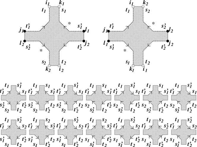
Figure 2: Diagrammatic representation of the contributions to the leading non-Gaussian correlator $W_{2}$ of equation (35), which involves four scattering matrices. The top left diagram has weight ${\cal F}(t_{1},t_{1}^{\prime};t_{2},t_{2}^{\prime};s_{1},s_{1}^{\prime};s_{2},s_{2}^{\prime})$, cf. equation (38). The top right diagram is obtained by interchange of two scattering matrices and has weight ${\cal F}(t_{1},t_{1}^{\prime};t_{2},t_{2}^{\prime};s_{2},s_{2}^{\prime};s_{1},s_{1}^{\prime})$. These two diagrams give all contributions to the cumulant $W_{2}$ in the absence of time-reversal symmetry. In the presence of time-reversal symmetry, the fourteen lower diagrams, corresponding to the reversal of one or more directions of the vertices, contribute as well.

The central result of this paper is a calculation of the cumulants $W_{1}$ and $W_{2}$ for time-dependent scattering. Details of the calculation are reported in appendix C. For the second moment $W_{1}$ we find

$$W_{1}^{ij;kl}(t,t^{\prime};s,s^{\prime}) = \delta(t-t^{\prime}-s+s^{\prime})\theta(t-t^{\prime})\left[\delta_{ik}\delta_{jl}{\cal D}(t,t^{\prime};s,s^{\prime})+\delta_{il}\delta_{jk}{\cal D}(t,t^{\prime};s^{\prime},s)\right],$$ (36)

with

$${\cal D}(\tau,\sigma;\tau^{\prime},\sigma^{\prime})=\exp\left[-N|\tau-\sigma|-{2\pi\over\Delta}\int_{0}^{|\tau-\sigma|}d\xi\left(V(\sigma+\eta\xi)-V(\sigma^{\prime}+\eta^{\prime}\xi)\right)\right.$$ (37)

$$\left.\mbox{}+2\sum_{j}\left[x_{j}(\sigma+\eta\xi)-x_{j}(\sigma^{\prime}+\eta^{\prime}\xi)\right]^{2}+\left[\eta\alpha(\sigma+\eta\xi)-\eta^{\prime}\alpha(\sigma^{\prime}+\eta^{\prime}\xi)\right]^{2}\right],$$

and $\eta=\mbox{sign}\,(\tau-\sigma)$, $\eta^{\prime}=\mbox{sign}\,(\tau^{\prime}-\sigma^{\prime})$. The first term in equation (36) is the analogue of the diffuson from standard diagrammatic perturbation theory, while the second term corresponds to the cooperon. For notational convenience, both terms are denoted by the same symbol ${\cal D}$. (Note that the order of the time arguments $s$ and $s^{\prime}$ is reversed in the second term of equation (36).) The leading non-Gaussian corrections are given by the cumulant $W_{2}$ for which we find

$$W_{2}^{i_{1}j_{1},i_{2}j_{2};k_{1}l_{1},k_{2}l_{2}}(t_{1},t_{1}^{\prime};t_{2},t_{2}^{\prime};s_{1},s_{1}^{\prime};s_{2},s_{2}^{\prime})=\theta(t_{1}-t_{1}^{\prime})\theta(t_{2}-t_{2}^{\prime})\theta(s_{1}-s_{1}^{\prime})\theta(s_{2}-s_{2}^{\prime})$$

$$\mbox{}\times\delta_{i_{1}k_{1}}\delta_{j_{1}l_{2}}\delta_{i_{2}k_{2}}\delta_{j_{2}l_{1}}\delta(t_{1}-t_{1}^{\prime}+t_{2}-t_{2}^{\prime}-s_{1}+s_{1}^{\prime}-s_{2}+s_{2}^{\prime})$$

$$\mbox{}\times{\cal F}(t_{1},t_{1}^{\prime};t_{2},t_{2}^{\prime};s_{1},s_{1}^{\prime};s_{2},s_{2}^{\prime})+\mbox{permutations}.$$ (38)

The “permutations” in equation (38) refer to one term corresponding to the permutation $(s_{1},s_{1}^{\prime},k_{1},l_{1})\leftrightarrow(s_{2},s_{2}^{\prime},k_{2},l_{2})$ of the third and fourth arguments of $W_{2}$ and fourteen more terms corresponding to the interchange of incoming and outgoing channel and time arguments within the second, third, and fourth argument of $W_{2}$. A diagrammatic representation of the cumulant (38) and the relevant perturbations is shown in figure 2. The kernel ${\cal F}$ reads

$${\cal F}(\tau_{1},\sigma_{1};\tau_{2},\sigma_{2};\tau_{1}^{\prime},\sigma_{1}^{\prime};\tau_{2}^{\prime},\sigma_{2}^{\prime})=\int d\xi\,{\cal D}(\sigma_{1}+\eta_{1}\xi,\sigma_{1};\sigma_{1}^{\prime}+\eta_{1}^{\prime}\xi,\sigma_{1}^{\prime})$$

$$\mbox{}\times{\cal D}(\tau_{2}-\tau_{1}^{\prime}+\sigma_{1}^{\prime}+\eta_{2}\xi,\sigma_{2};\tau_{2}^{\prime}-\tau_{1}+\sigma_{1}+\eta_{2}^{\prime}\xi,\sigma_{2}^{\prime})$$

$$\mbox{}\times{\cal D}(\tau_{1},\sigma_{1}+\eta_{1}\xi;\tau_{2}^{\prime},\tau_{2}^{\prime}-\tau_{1}+\sigma_{1}+\eta_{2}^{\prime}\xi)$$

$$\mbox{}\times{\cal D}(\tau_{2},\tau_{2}-\tau_{1}^{\prime}+\sigma_{1}^{\prime}+\eta_{2}\xi;\tau_{1}^{\prime},\sigma_{1}^{\prime}+\eta_{1}^{\prime}\xi)$$

$$\mbox{}\times\left\{N+4\sum_{m}[x_{m}(\sigma_{1}+\eta_{1}\xi)-x_{m}(\tau_{2}^{\prime}-\tau_{1}+\sigma_{1}+\eta_{2}^{\prime}\xi)]\right.$$

$$\left.\ \ \mbox{}\times[x_{m}(\sigma_{1}^{\prime}+\eta_{1}^{\prime}\xi)-x_{m}(\tau_{2}-\tau_{1}^{\prime}+\sigma_{1}^{\prime}+\eta_{2}\xi)]-\delta(\xi-|\tau_{1}-\sigma_{1}|)\right.$$

$$\ \ \left.\mbox{}-\delta(\xi-|\tau_{1}^{\prime}-\sigma_{1}^{\prime}|)+2[\eta_{1}\alpha(\sigma_{1}+\eta_{1}\xi)-\eta_{2}^{\prime}\alpha(\tau_{2}^{\prime}-\tau_{1}-\sigma_{1}+\eta_{2}^{\prime}\xi)]\right.$$

$$\left.\ \ \mbox{}\times[\eta_{1}^{\prime}\alpha(\sigma_{1}^{\prime}+\eta_{1}^{\prime}\xi)-\eta_{2}\alpha(\tau_{2}-\tau_{1}^{\prime}+\sigma_{1}^{\prime}+\eta_{2}\xi)]\vphantom{\sum_{m}}\right\},$$ (39)

where we abbreviated $\eta_{1}=\mbox{sign}\,(\tau_{1}-\sigma_{1})$, $\eta_{2}=\mbox{sign}\,(\tau_{2}-\sigma_{2})$, $\eta_{1}^{\prime}=\mbox{sign}\,(\tau_{1}^{\prime}-\sigma_{1}^{\prime})$, and $\eta_{2}^{\prime}=\mbox{sign}\,(\tau_{2}^{\prime}-\sigma_{2}^{\prime})$. Note that equations (36)–(39) cover both the cases with and without time-reversal symmetry through the explicit dependence on the magnetic flux $\alpha$. If time-reversal symmetry is fully broken, all permutations in equation (38) that involve the interchange of incoming and outgoing channels, corresponding to the fourteen lower diagrams in figure 2, vanish, and only the first two diagrams in figure 2 remain. Partial integration of the intermediate time $\xi$ allows one to rewrite terms between brackets $\{\ldots\}$ in equation (39), see appendix C for details. Finally, one verifies that the result (26) is recovered for $\alpha=0$ and $\alpha\gg 1$, corresponding to presence and absence of time-reversal symmetry, when the parameters $x_{j}$ and $\alpha$ do not depend on time.

4 Applications

In order to illustrate the use of equations (36)–(39), we return to the example of section 2 and consider transport through a chaotic quantum dot coupled to two electrons reservoirs by means of ballistic point contacts with $N_{1}$ and $N_{2}$ channels, respectively. The scattering matrix of the quantum dot has dimension $N=N_{1}+N_{2}$. The current through the dot is defined as a linear combination of the of the currents through the two point contacts,

$${\bf I}(t) = e\sum_{i,j=1}^{N}\left({\bf a}_{i}^{\dagger}(t){\Lambda}_{ij}{\bf a}_{j}(t)-{\bf b}_{i}^{\dagger}(t)\Lambda_{ij}{\bf b}_{j}(t)\right),$$ (40)

where the $N\times N$ matrix $\Lambda$ was defined in equation (9) and the operators ${\bf a}_{i}(t)$ and ${\bf b}_{i}(t)$ are annihilation operators for incoming and outgoing states in channel $i=1,\ldots,N$ in the leads, respectively, see section 3. The advantage of the definition (40) for the current through the quantum dot, instead of a definition where the current through one of the contacts is used, is that it simplifies the ensemble average taken below. Both definitions of the current give the same result for the quantity of interest, the integral of ${\bf I}(t)$ over a large time interval $t_{\rm i}<t<t_{\rm f}$.

The electron distribution function for the electrons entering the quantum dot from the leads is given by the Fourier transform $f(t)$ of the Fermi function in the corresponding electron reservoir [57, 58, 59],

$$\overline{{\bf a}_{j}^{\dagger}(t^{\prime}){\bf a}_{i}^{\vphantom{\dagger}}(t)} = f_{ij}(t^{\prime}-t),$$

$$\overline{{\bf a}_{j}^{\vphantom{\dagger}}(t^{\prime}){\bf a}_{i}^{\dagger}(t)} = \tilde{f}_{ij}(t-t^{\prime}),$$ (41)

where we defined

$$f_{ij}(t) = \delta_{ij}\int{d\varepsilon\over 2\pi\hbar}\frac{\rme^{\rmi\varepsilon t/\hbar}}{\rme^{(\varepsilon-\mu_{i})/kT}+1}$$

$$= \delta_{ij}\frac{ikT\rme^{\rmi\mu_{i}t/\hbar}}{2\hbar\sinh(\pi kTt/\hbar)},$$

$$\tilde{f}_{ij}(t) = \delta_{ij}\delta(t)-f_{ij}(t).$$ (42)

Here $\mu_{i}$ is the chemical potential of reservoir $1$ for $1\leq i\leq N_{1}$ and the chemical potential of reservoir $2$ for $N_{1}<i\leq N$.

Substitution of equations (41) and (17) into equation (40) allows us to calculate the time-averaged expectation value of the current through the quantum dot for a time interval $t_{\rm i}<t<t_{\rm f}$,

$$I={2e\over t_{\rm f}-t_{\rm i}}\int_{t_{\rm i}}^{t_{\rm f}}dt\int dt_{1}dt_{2}\tr\left[\delta(t-t_{1})\Lambda\delta(t-t_{2})-{\cal S}^{\dagger}(t_{1},t)\Lambda{\cal S}(t,t_{2})\right]f(t_{1}-t_{2}).$$ (43)

(A factor two has been added to account for spin degeneracy. The time interval $t_{\rm i}<t<t_{\rm f}$ during which charge is measured is taken to be the largest time scale in the problem.)

In the absence of a source-drain voltage, equation (43) describes the current that is “pumped” by the time-dependent potential in the dot,

$$I_{\rm pump} = -{2e\over t_{\rm f}-t_{\rm i}}\int_{t_{\rm i}}^{t_{\rm f}}dt\int dt_{1}dt_{2}\tr{\cal S}^{\dagger}(t_{1},t)\Lambda{\cal S}(t,t_{2})f_{\rm eq}(t_{1}-t_{2}),$$ (44)

where $f_{\rm eq}$ is the Fourier transform of the Fermi function. Equation (44) was first derived in reference [35]; it reduces to the current formulae of references [53] and [54] in the adiabatic limit, where the time dependence of the potential of the quantum dot is slow compared to the dwell time in the quantum dot. At small bias voltage, there is a current proportional to the bias, $I=GV$, where $G$ is the (time-averaged) conductance of the dot. The conductance $G$ can be calculated from equation (43) by setting $\mu_{i}=\Lambda_{ii}eV$ and then linearizing in $V$ [22],

$$G = {2e^{2}\over h}\left[{N_{1}N_{2}\over N}-{2\pi\rmi\over t_{\rm f}-t_{\rm i}}\int_{t_{\rm i}}^{t_{\rm f}}dt\int dt_{1}dt_{2}(t_{1}-t_{2})\tr\Lambda{\cal S}(t,t_{1})\Lambda{\cal S}^{\dagger}(t_{2},t)f_{\rm eq}(t_{1}-t_{2})\right].$$ (45)

Here $f_{\rm eq}$ is the Fermi function in the absence of the external bias. For time-independent transport, equation (45) is equal to the Landauer formula (8).

Conductance. The ensemble average and the variance of the conductance $G$ for a quantum dot with a shape depending on a single time-dependent parameter $x$ was calculated by Vavilov and Aleiner using the Hamiltonian approach [22]. Using the scattering matrix correlator (34), their result for $\langle G\rangle$ is easily reproduced and generalized to arbitrary values of the (time-independent) magnetic field,

$$\langle G\rangle={2e^{2}N_{1}N_{2}\over hN}+\delta G;$$ (46)

$$\delta G=-{2e^{2}N_{1}N_{2}\over hN(t_{\rm f}-t_{\rm i})}\int_{t_{\rm i}}^{t_{\rm f}}dt\int_{0}^{\infty}d\tau$$

$$\mbox{}\times\exp\left[-(N+4\alpha^{2})\tau-2\int_{0}^{\tau}d\tau_{1}(x(t-\tau+\tau_{1})-x(t-\tau_{1}))^{2}\right].$$ (47)

The correction term $\delta G$ of equation (47) is the weak localization correction; it results from the constructive interference of time-reversed trajectories. The presence of a time-dependent potential breaks time-reversal symmetry and suppresses the weak localization correction. Vavilov and Aleiner investigated the case $x(t)=\delta x\cos(\omega t)$ of a harmonic time dependence for the parameter $x$ in detail. In that case, the suppression of weak localization increases with increasing frequencies and saturates at a value

$$\delta G=-{2e^{2}N_{1}N_{2}\over N^{2}h}\times\left\{\begin{array}[]{ll}\left[1-{2(\delta x)^{2}\over N+4\alpha^{2}\vphantom{M^{M}_{M}}}\right]&\mbox{if $(\delta x)^{2}\ll N+4\alpha^{2}$},\\ \sqrt{N+4\alpha^{2}\vphantom{M^{M}_{M}}\over 4(\delta x)^{2}}&\mbox{if $(\delta x)^{2}\gg N+4\alpha^{2}$,}\end{array}\right.$$ (48)

for frequencies $\hbar\omega\gtrsim N\Delta$ [22]. (Applicability of random matrix theory requires that $\omega\ll 1/\tau_{\rm erg}$, where $\tau_{\rm erg}$ is the time for ergodic exploration of the quantum dot.) If the fluctuations of the parameter $x$ are fast and random on the scale $2\pi\hbar/N\Delta$ of the delay time in the dot, they may be considered Gaussian white noise,

$$\langle x(t)x(t^{\prime})\rangle={1\over 4}\gamma\delta(t-t^{\prime}).$$ (49)

In that case, the exponent in equation (47) can be averaged separately, and one finds the result

$$\delta G=-{2e^{2}N_{1}N_{2}\over hN(N+4\alpha^{2}+\gamma)}.$$ (50)

The same suppression of weak localization was obtained previously to describe the decohering effect of the coupling to an external bath [60, 61, 62]. Note that the strong-perturbation asymptote for white noise is different from the strong-perturbation asymptote for fast harmonic variations of the dot’s shape. The cause for this difference is the existence of small time windows in which time-reversal symmetry is not violated near times $t$ with $\cos(\omega t)=\pm 1$ for harmonic variations $\propto\cos(\omega t)$, while for a random time dependence of $x(t)$ no such special times around which time-reversal symmetry is preserved exist [25, 26].

Similarly the variance of the conductance can also be expressed in terms of the correlator (34). (As in the time-independent case, the non-Gaussian correlator (38) does not contribute to the variance of the conductance.) We refer to reference [23] for the detailed expression for $\mbox{var}\,G$ and an analysis of the effect of a harmonic time dependence of the shape function $x(t)$. Conductance fluctuations for the case when $x(t)$ is a sum of two harmonics with different frequencies were considered by Kravtsov and Wang [25].

Figure 3: Diagrams representing the two contributions to the variance of the pumped current. Following the notation of reference [36], dotted lines correspond to the scattering matrix ${\cal S}$, thick solid lines correspond to the fixed matrices $\Lambda$ and $f$, and thin solid lines correspond to the Kronecker delta’s in the average over the ensemble of scattering matrices.

Pumped current. To first order in the pumping frequency $\omega$, the current in the absence of a source-drain voltage is nonzero only if two or more parameters $x_{j}$ that determine the dot’s shape are varied independently. Even then, the ensemble average of the pumped current is zero, and the first nonzero moment is $\langle I^{2}\rangle$. The ensemble average $\langle I^{2}\rangle$ was calculated in reference [53] for small pumping amplitudes $x_{1}(t)=\delta x_{1}\sin(\omega t)$, $x_{2}=\delta x_{2}\sin(\omega t+\phi)$,

$$\langle I^{2}\rangle^{1/2}={e\omega\delta x_{1}\delta x_{2}\over 2\pi N}\sin\phi,$$ (51)

independent of the presence or absence of a magnetic field. The case of pumping amplitudes of arbitrary strength was considered in reference [34].

Beyond the adiabatic regime, one time-dependent parameter is sufficient to generate a finite current through the dot [63, 52]. The second moment $\langle I^{2}\rangle$ in that most general case was first calculated in reference [35], using the random Hamiltonian approach. The second moment, which involves an average over four scattering matrix elements, can also be obtained in the random scattering matrix approach, using equations (36)–(39) of the previous section. We then find that there are two contributions to $\langle I_{\rm pump}^{2}\rangle$: one contribution with two Gaussian contractions of scattering matrices (giving a factor $W_{1}^{2}$) and one contribution which involves a correlator of four scattering matrices (giving a factor $W_{2}$). Diagrams representing these two contributions are shown in figure 3. Adding both contributions, we find

$$\langle I_{\rm pump}^{2}\rangle = {8e^{2}N_{1}N_{2}\over N(t_{\rm f}-t_{\rm i})^{2}}\int_{t_{\rm i}}^{t_{\rm f}}dtdt^{\prime}\int_{0}^{\infty}d\tau d\xi d\xi^{\prime}\int_{-\tau}^{\tau}d\tau^{\prime}f_{\rm eq}(2\tau^{\prime})f_{\rm eq}(-2\tau^{\prime})$$ (52)

$$\mbox{}\times{\cal D}(t,t-\tau-\tau^{\prime};t^{\prime},t^{\prime}-\tau-\tau^{\prime}){\cal D}(t^{\prime},t^{\prime}-\tau+\tau^{\prime};t,t-\tau+\tau^{\prime})$$

$$\mbox{}\times{\cal D}(t-\tau-\tau^{\prime},t-\tau-\tau^{\prime}-\xi;t-\tau+\tau^{\prime},t-\tau+\tau^{\prime}-\xi)$$

$$\mbox{}\times{\cal D}(t^{\prime}-\tau+\tau^{\prime},t^{\prime}-\tau+\tau^{\prime}-\xi^{\prime};t^{\prime}-\tau-\tau^{\prime},t^{\prime}-\tau-\tau^{\prime}-\xi^{\prime})$$

$$\mbox{}\times\left[(\delta(\xi)-N)(\delta(\xi^{\prime})-N)+4\sum_{m}(x_{m}(t^{\prime}-\tau+\tau^{\prime})-x_{m}(t^{\prime}-\tau-\tau^{\prime}))\right.$$

$$\left.\ \ \ \ \mbox{}\times(x_{m}(t-\tau+\tau^{\prime})-x_{m}(t-\tau-\tau^{\prime}))\vphantom{\sum_{m}}\right],$$

independent of the value of the magnetic field. Using equation (71) of appendix C to express the delta functions in terms of the functions $x_{m}(t)$ and a total derivative of ${\cal D}$, performing partial integrations, and shifting $t\to t-\tau$, $t^{\prime}\to t^{\prime}-\tau$, this can be rewritten as

$$\langle I_{\rm pump}^{2}\rangle={32e^{2}N_{1}N_{2}\over N(t_{\rm f}-t_{\rm i})^{2}}\int_{0}^{\infty}d\tau d\xi d\xi^{\prime}\int_{-\tau}^{\tau}d\tau^{\prime}\int_{t_{\rm i}-\tau}^{t_{\rm f}-\tau}dtdt^{\prime}f_{\rm eq}(2\tau^{\prime})f_{\rm eq}(-2\tau^{\prime})$$

$$\mbox{}\times{\cal D}(t+\tau,t-\tau^{\prime};t^{\prime}+\tau,t^{\prime}-\tau^{\prime}){\cal D}(t-\tau^{\prime},t-\tau^{\prime}-\xi;t+\tau^{\prime},t+\tau^{\prime}-\xi)$$

$$\mbox{}\times{\cal D}(t^{\prime}+\tau,t^{\prime}+\tau^{\prime};t+\tau,t+\tau^{\prime}){\cal D}(t^{\prime}+\tau^{\prime},t^{\prime}+\tau^{\prime}-\xi^{\prime};t^{\prime}-\tau^{\prime},t^{\prime}-\tau^{\prime}-\xi^{\prime})$$

$$\mbox{}\times\left[\sum_{m,n}\left(\sum_{\pm}\pm x_{m}(t\pm\tau^{\prime}-\xi)\right)^{2}\left(\sum_{\pm}\pm x_{n}(t\pm\tau^{\prime}-\xi^{\prime})\right)^{2}\right.$$

$$\left.\ \ \mbox{}+\sum_{m}\left(\sum_{\pm}\pm x_{m}(t^{\prime}-\tau\pm\tau^{\prime})\right)\left(\sum_{\pm}\pm x_{m}(t-\tau\pm\tau^{\prime})\right)\right].$$ (53)

This expression agrees with the result found by Vavilov, Ambegaokar, and Aleiner [35]. We refer to reference [35] for a detailed analysis of equation (53) for the limiting cases of adiabatic pumping and high-frequency pumping with one and two time-dependent parameters.

Noise. The current noise is defined as the variance of the charge transmitted through the quantum dot in the time interval $t_{\rm i}<t<t_{\rm f}$

$$S={1\over t_{\rm f}-t_{\rm i}}\int dtdt^{\prime}\left(\overline{{\bf I}(t){\bf I}(t^{\prime})}-\overline{{\bf I}(t)}\,\overline{{\bf I}(t^{\prime})}\right).$$ (54)

As in equation (41), $\overline{\cdots}$ denotes a quantummechanical or thermal average, not an ensemble average. Performing the quantummechanical and thermal average over the incoming states [57, 58, 59], the noise power $S$ can be calculated as

$$S={2e^{2}\over t_{\rm f}-t_{\rm i}}\int_{t_{\rm i}}^{t_{\rm f}}dtdt^{\prime}\int dt_{1}dt_{2}dt^{\prime}_{1}dt^{\prime}_{2}\tr\left[\left({\cal S}^{\dagger}(t_{1},t)\Lambda{\cal S}(t,t_{2})-\delta(t_{1}-t)\Lambda\delta(t-t_{2})\right)\right.$$

$$\left.\mbox{}\times\tilde{f}(t_{1}^{\prime}-t_{2})\left({\cal S}^{\dagger}(t_{1}^{\prime},t^{\prime})\Lambda{\cal S}(t^{\prime},t_{2}^{\prime})-\delta(t_{1}^{\prime}-t^{\prime})\Lambda\delta(t^{\prime}-t_{2}^{\prime})\right)f(t_{1}-t_{2}^{\prime})\right].$$

(A factor two has been added to account for spin degeneracy.) In the absence of a time-dependent potential, Equation (4) represents the sum of Nyquist noise and shot noise [64]. With time-dependence, it contains an extra contribution to the noise that is caused by the time dependence of the potential in the quantum dot [65, 66, 67, 68, 69, 37].

Averaging equation (4) for an ensemble of chaotic quantum dots, we find

$$\langle S\rangle=S^{N}+S^{S}+S^{P},$$

$$S^{N}=2kTh\langle G\rangle,$$

$$S^{S}=eVh\langle G\rangle{N_{1}N_{2}\over 2\pi N^{2}}\left(\coth\frac{eV}{2kT}-\frac{2kT}{eV}\right),$$

$$S^{P}={e^{2}N_{1}N_{2}(kT/\hbar)^{2}\over 2N(t_{\rm f}-t_{\rm i})}\int_{t_{\rm i}}^{t_{\rm f}}dtdt^{\prime}\left({1\over N^{2}}-\left[\int_{0}^{\infty}{\cal D}(t,t-\xi;t^{\prime},t^{\prime}-\xi)d\xi\right]^{2}\right)$$

$$\mbox{}\times\frac{N^{2}-2({N_{1}^{2}+N_{2}^{2}})\sin^{2}[eV(t-t^{\prime})/2\hbar]}{\sinh^{2}[\pi kT(t-t^{\prime})/\hbar]},$$ (55)

where $\langle G\rangle$ is the average (time-dependent) conductance, see equation (46), and $V=(\mu_{1}-\mu_{2})/e$ the bias voltage. The above ensemble averages for the Nyquist noise and shot noise are the same as the noise power found in the absence of a time-dependent potential [70], up to an eventual weak localization correction. The extra noise generated by the time-dependence of the dot shape is fully described by the term $S^{P}$. In the adiabatic regime $\hbar\omega\ll N\Delta$, the pumping noise can be written as

$$S^{P}=\frac{e^{2}N_{1}N_{2}(kT/\hbar)^{2}}{2N(t_{\rm f}-t_{\rm i})}\int_{t_{\rm i}}^{t_{\rm f}}dt^{\prime}dt\left[{1\over N^{2}}-\left(\frac{1}{N+2\sum_{m}(x_{m}(t)-x_{m}(t^{\prime}))^{2}}\right)^{2}\right]$$

$$\mbox{}\times\frac{N^{2}-2({N_{1}^{2}+N_{2}^{2}})\sin^{2}[eV(t-t^{\prime})/2\hbar]}{\sinh^{2}[\pi kT(t-t^{\prime})/\hbar]},$$ (56)

In the absence of a bias voltage, $eV=0$, Equation (4) has been analyzed in detail by Vavilov and the authors in reference [37]. For one time-dependent parameter $x(t)=\delta x\cos(\omega t)$ it is found that

$$S^{P}={\omega e^{2}N_{1}N_{2}\over\pi^{2}N^{2}}\left\{\begin{array}[]{ll}2\pi(\delta x)^{2}\left(\coth{\hbar\omega\over 2kT}-{2kT\over\hbar\omega}\right)_{\vphantom{M}}^{\vphantom{M}},&\mbox{if $(\delta x)^{2}\ll N\max(1,k^{2}T^{2}/\hbar^{2}\omega^{2})$,}\\ \vphantom{\left(M^{M}_{M}\right)}3|\delta x|N^{1/2},&\mbox{if $(\delta x)^{2}\gg N\max(1,k^{2}T^{2}/\hbar^{2}\omega^{2})$.}\end{array}\right.$$ (59)

An applied bias voltage has an effect on the pumping noise $S^{P}$ only if $eV\gtrsim\max(\hbar\omega,kT,\hbar\omega|\delta x|/N^{1/2})$. And even then, the effect of the applied bias is limited to a reduction of $S^{P}$ by a numerical factor $2N_{1}N_{2}/N^{2}$. In this respect, the effect of an external bias on the pumping noise is much weaker than that of temperature, which tends to suppress $S^{P}$ as soon as $kT\gtrsim\hbar\omega\max(1,|\delta x|/N^{1/2})$ [37].

5 Conclusion

In summary, in this paper we have extended the scattering approach of the random-matrix theory of quantum transport to the case of scattering from a chaotic quantum dot with a time-dependent potential. We addressed the limit that the number of channels $N$ coupling the dot to the electron reservoirs is large. In this limit, the elements of the scattering matrix have a distribution that is almost Gaussian, with non-Gaussian corrections that are small as $N$ becomes large. We calculated the second moment, which defines the Gaussian part of the distribution, and the fourth cumulant, which characterizes the leading non-Gaussian corrections.

The advantage of the scattering matrix approach is that, once the scattering matrix distribution is calculated, the computation of transport properties is a matter of mere quadrature. As an example, we calculated the conductance of a quantum dot with a time-dependent potential or the current pumped through the dot in the absence of an external bias, and found agreement with previous calculations of Vavilov et al. that were based on the Hamiltonian approach [22, 23, 35]. The results derived here were used for the calculation of the current noise generated by the time-dependence of the potential in the quantum dot by Vavilov and the authors [37]. The current noise in the presence of both a time-dependent potential in the dot and a bias voltage was studied here.

Whereas the first four moments of the scattering matrix distribution that we calculated here are sufficient for the calculation of most transport properties — most transport properties are quadratic or quartic in the scattering matrix —, we need to point out that there are observables that cannot be calculated with the results presented here. First, in the presence of one or more superconducting contacts, (averaged) transport properties may still depend on higher cumulants of the distribution, despite the fact that these are small by additional factors of $1/N$ [11]. Second, the results presented here fail to quantitatively describe transport properties for very small $N$, which can have strongly non-Gaussian distributions. Further research in these directions is necessary.

Appendix A Nonideal contacts

Nonideal contacts are characterized by channels that have a transmission coefficient $\Gamma_{j}$ smaller than unity, $j=1,\ldots,N$. The imperfect transmission of the contacts is characterized by an $N\times N$ reflection matrix $r_{c}(t,t^{\prime})$, for which we take the simple form

$$r_{c}(t,t^{\prime})=(1-\Gamma)^{1/2}\delta(t-t^{\prime}),$$ (60)

where $\Gamma$ is an $N\times N$ diagonal matrix containing the transmission coefficients $\Gamma_{j}$ on the diagonal. The direct backscattering from the contacts is fast compared to the scattering that involves ergodic exploration of the dot, hence the delta function $\delta(t-t^{\prime})$ in equation (60). In order to describe time dependent scattering with nonideal leads, we use a modification of the stub model of equation (28) [71, 20],

$${\cal S} = r_{c}+\Gamma^{1/2}S^{\rm fl}\Gamma^{1/2},\ \ S^{\rm fl}=P{\cal U}(1-R{\cal U})^{-1}P^{\dagger},$$ (61)

$$R = Q^{\dagger}\rme^{-2\pi\rmi H/M\Delta}Q-P^{\dagger}r_{c}P.$$ (62)

The first term in equation (61) takes into account the direct backscattering at the contact for electrons coming in from the reservoirs, whereas the extra term in equation (62) describes backscattering at the contact for electrons coming from the dot. The additional factors $\Gamma^{1/2}$ in the second term of equation (61) account for the decreased transmission probability for entering or exiting the quantum dot. With the inclusion of reflection in the contacts as in equation (61), the scattering matrix approach for time-independent scattering was proven to be fully equivalent to the Hamiltonian approach with arbitrary coupling to the leads [20]. The corresponding distribution of the scattering matrix ${\cal S}$ for time-independent scattering is known as the Poisson kernel [19].

Like in the case of ideal leads, the distribution of the elements of the scattering matrix ${\cal S}$ for a quantum dot with nonideal leads is almost Gaussian, with non-Gaussian corrections that are small if $N\gg 1$. The main difference with the case of an ideal contact is that, as a result of the direct reflection from the contact, the average of ${\cal S}$ is nonzero for a nonideal contact. The fluctuations of ${\cal S}$ around the average are described by ${\cal S}^{\rm fl}$, cf. equation (61). In order to find the distribution of ${\cal S}^{\rm fl}$, we note that the expression (61) for ${\cal S}^{\rm fl}$ is formally equivalent to the stub model equation (28) used to describe time-dependent scattering from a quantum dot with ideal contacts. Hence we conclude that the moments of ${\cal S}^{\rm fl}$ can be obtained directly from the results for the case of ideal contacts, see section 3 and appendix C, provided we substitute equation (62) for the matrix $R$. This amounts to the replacement ${\cal S}\to{\cal S}^{\rm fl}$ in the final results (36)–(39), $N\to\sum_{j}\Gamma_{j}$ in equation (37), and $N\to\sum_{j}\Gamma_{j}^{2}$ in equation (39).

Appendix B Correlators for time-independent scattering

The scattering matrix correlators for time-independent scattering serve as input for the calculation of the correlators for time-dependent scattering. They can be calculated using the Hamiltonian approach (see references [12, 44, 45]), or, alternatively, in the scattering matrix approach, using a time-independent version of the “stub model” of section 3. Following the latter method, the scattering matrix ${\cal S}$ is written as [46]

$${\cal S}(\varepsilon)=P{\cal U}(1-R{\cal U})^{-1}P^{\dagger},\ \ R=Q^{\dagger}\rme^{2\pi\rmi\varepsilon/M\Delta}Q.$$ (63)

Here the matrices $P$ and $Q$ are as in equation (28), whereas ${\cal U}$ is an $M\times M$ unitary matrix taken from the circular orthogonal ensemble or circular unitary ensemble of random matrix theory, depending on the presence or absence of time-reversal symmetry. The picture underlying equation (63) is that a stub with $M-N$ scattering channels is attached to the chaotic quantum dot as in figure 1, such that the dwell time in the stub is much larger than the dwell time in the dot, but much smaller than the total dwell time in the combined dot-stub system. The first condition implies that the $M\times M$ scattering matrix of the chaotic dot (without stub) may be taken energy independent, and distributed according to the appropriate circular ensemble from random matrix theory. The total scattering matrix ${\cal S}$ then acquires its energy dependence through the energy dependence of the $(M-N)\times(M-N)$ reflection matrix $R$ of the stub. The second condition, which requires $M\gg N$, ensures that the dot plus stub system is explored ergodically before an electron escapes into the lead, so that the spatial separation of the energy dependence (stub) and chaotic scattering (dot)) does not affect the correlators of the scattering matrix ${\cal S}$.

Using the diagrammatic technique of reference [36] to average over the random unitary matrix ${\cal U}$, we find that the second moment $W_{1}$ is given by

$$W_{1}^{ij;kl}(\varepsilon;\varepsilon^{\prime}) = {1\over M-\tr R(\varepsilon)R^{\dagger}(\varepsilon^{\prime})}\times\left\{\begin{array}[]{ll}(\delta_{ik}\delta_{jl}+\delta_{il}\delta_{jk})&\mbox{with TRS},\\ \delta_{ik}\delta_{jl}&\mbox{without TRS}.\end{array}\right.$$ (66)

Substitution of equation (63) for $R$ gives equation (14) of section 3. Note that equation (14) is valid in the semiclassical limit of large $N$ only. Within the diagrammatic technique this follows from the observation that for large $N$ the only contributions to $W_{1}$ are the “ladder” and “maximally crossed” diagrams, whereas for small $N$ more contributions exist and a non-perturbative calculation is needed to calculate the scattering matrix correlator [36]. The correlator $W_{1}(\varepsilon,\varepsilon^{\prime})$ was calculated by Verbaarschot et al. in reference [12] for arbitrary $N$ using the Hamiltonian approach and the supersymmetry technique.

For the cumulant $W_{2}$ we find in the absence of time-reversal symmetry

$$W_{2}^{i_{1}j_{1},i_{2}j_{2};k_{1}l_{1},k_{2}l_{2}}(\varepsilon_{1},\varepsilon_{2};\varepsilon_{1}^{\prime},\varepsilon_{2}^{\prime})=-\left(\delta_{i_{1}k_{1}}\delta_{j_{1}l_{2}}\delta_{i_{2}k_{2}}\delta_{j_{2}l_{1}}+\delta_{i_{1}k_{1}}\delta_{j_{1}l_{2}}\delta_{i_{2}k_{2}}\delta_{j_{2}l_{1}}\right)$$

$$\mbox{}\times[M-\tr R(\varepsilon_{1})R(\varepsilon_{2})R^{\dagger}(\varepsilon_{1}^{\prime})R^{\dagger}(\varepsilon_{2}^{\prime})]$$

$$\mbox{}\times[M-\tr R(\varepsilon_{1})R(\varepsilon_{1}^{\prime})]^{-1}[M-\tr R(\varepsilon_{2})R(\varepsilon_{1}^{\prime})]^{-1}$$

$$\mbox{}\times[M-\tr R(\varepsilon_{1})R(\varepsilon_{2}^{\prime})]^{-1}[M-\tr R(\varepsilon_{2})R(\varepsilon_{2}^{\prime})]^{-1}.$$ (67)

In the presence of time-reversal symmetry, fourteen terms corresponding to the permutations $i_{2}\leftrightarrow j_{2}$, $k_{1}\leftrightarrow l_{1}$, and $k_{2}\leftrightarrow l_{2}$ have to be added. Equation (15) is recovered upon substitution of equation (63) for $R$.

Appendix C Correlators for time-dependent scattering

In this appendix we present the derivations of equations (36)–(39).

We first calculate the second moment $W_{1}$ of the scattering matrix distribution, equations (36) and (37). To find $W_{1}$ we use equation (28) to expand ${\cal S}$ in powers of ${\cal U}$ and $R$ and then average over ${\cal U}$. In the limit of large $M$ and large $N$, that average can be done using the cumulants (24) and (26) and the diagrammatic rules of reference [36]. This calculation is similar to the standard diagrammatic perturbation theory: the matrices ${\cal U}$, ${\cal U}^{\dagger}$, and $R(t)$ play the role of the unperturbed retarded and advanced Green functions and the random potential, respectively.

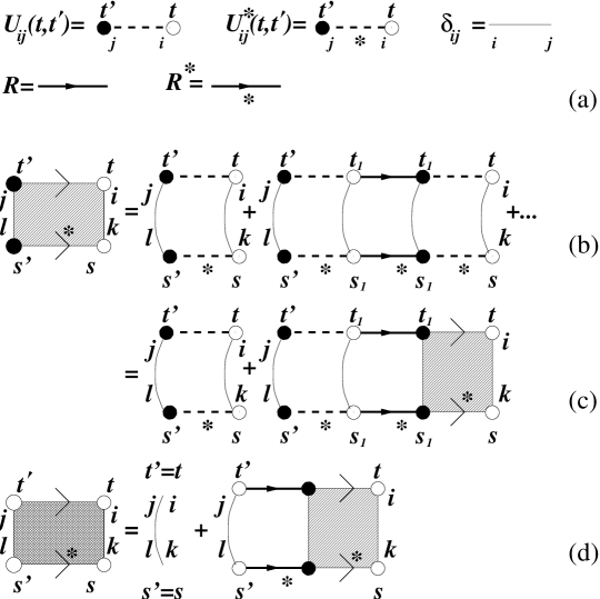
Figure 4: (a) Notations, following reference [36]. (b) Calculation of the kernel $D(t,t^{\prime};s,s^{\prime})$. (c) Diagrammatic representation of the Dyson equation (69) for $D(t,t-\tau;s,s-\tau)$, with $t^{\prime}=t-\tau$, $t_{1}=t-\tau_{1}$, $s^{\prime}=s-\tau$, and $s_{1}=s-\tau_{1}$. (d) Diagrammatic representation of the differential equation (71) for $D(t,t-\tau;s,s-\tau)$. Left hand side: $(M+\partial_{\tau})D(t,t-\tau;s,s-\tau)$; Right hand side: $\delta(\tau)+\tr R(t-\tau)R^{\dagger}(s-\tau)D(t,t-\tau;s,s-\tau)$.

Performing the average over ${\cal U}$ this way, we find that, to leading order in $M^{-1}$ and $N^{-1}$, the cumulant $W_{1}$ is dominated by two leading contributions: the “ladder diagram” of figure 4 and the “maximally crossed diagram” of figure 5. Since every factor in these two diagrams involves equal time differences for ${\cal S}$ and ${\cal S}^{*}$, we conclude that this contribution to $W_{1}$ is nonzero only if $t-t^{\prime}=s-s^{\prime}$, cf. equation (24). Further, we conclude that the ladder diagram gives a nonzero contribution only if $i=k$ and $j=l$, while the maximally crossed diagram contributes when $i=l$ and $j=k$.

We first consider the contribution of the ladder diagram, which we write as

$$\delta_{ik}\delta_{jl}\delta(t-t^{\prime}-s+s^{\prime})D(t,t^{\prime};s,s^{\prime}),$$ (68)

where the kernel $D$ is the equivalent of the “diffuson” from standard diagrammatic perturbation theory. Note that, in view of the delta function in equation (68), the kernel $D$ depends on three arguments, not on four. For notational convenience, we prefer, however, to continue to use the two initial times $t^{\prime}$ and $s^{\prime}$ and the two final times $t$ and $s$ to denote the time-arguments of $D$.

Considering the ladder diagrams to all orders, the diffuson $D$ is found to obey the Dyson equation

$$D(t,t-\tau;s,s-\tau)=\theta(\tau)\rme^{-M\tau}+\theta(\tau)\int_{0}^{\tau}d\tau_{1}D(t,t-\tau_{1};s,s-\tau_{1})\,$$

$$\mbox{}\times\tr R(t-\tau_{1})R^{\dagger}(s-\tau_{1})\rme^{-M(\tau-\tau_{1})}.$$ (69)

The solution of equation (69) is

$$D(t^{\prime}+\tau,t^{\prime};s^{\prime}+\tau,s^{\prime}) = \theta(\tau)\exp\left[-\int_{0}^{\tau}d\tau_{1}\left(M-\tr R(t^{\prime}+\tau_{1})R^{\dagger}(s^{\prime}+\tau_{1})\right)\right],$$ (70)

where we used that $D=0$ if $\tau<0$. Substitution of $R=\exp(2\pi H/\Delta)$ reproduces the first term in the result (36). For future use, we note that the function $D$ of equation (70) obeys the differential equations

$${{\partial\over\partial\tau}D(t,t-\tau;s,s-\tau)}=\delta(\tau)-\left[M-\tr R(t-\tau)R^{\dagger}(s-\tau)\right]D(t,t-\tau;s,s-\tau),$$ (71)

$${{\partial\over\partial\tau}D(t^{\prime}+\tau,t^{\prime};s^{\prime}+\tau,s^{\prime})}=\delta(\tau)-\left[M-\tr R(t^{\prime}+\tau)R^{\dagger}(s^{\prime}+\tau)\right]D(t^{\prime}+\tau,t^{\prime};s^{\prime}+\tau,s^{\prime}).$$

(72)

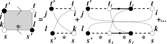
Figure 5: Diagram representing the kernel $C(t,t^{\prime};s,s^{\prime})$ of equation (74).

Calculation of the contribution of the maximally crossed diagram proceeds in an analogous way. This contribution reads

$$\delta(t-t^{\prime}-s+s^{\prime})\delta_{il}\delta_{jk}C(t,t^{\prime};s,s^{\prime}),$$ (73)

where the analogue of the Cooperon is given by

$$C(t^{\prime}+\tau,t^{\prime};s^{\prime}+\tau,s^{\prime})=\theta(\tau)\exp\left[{-\int_{0}^{\tau}d\tau_{1}\left(M-\tr R(t^{\prime}+\tau_{1})R^{\dagger}(s^{\prime}+\tau-\tau_{1})\right)}\right].$$ (74)

Substitution of $R=\exp(2\pi H/\Delta)$ gives the second term of equation (36).

We now turn to the four scattering-matrix correlator (35), which is the equivalent of the Hikami box in standard diagrammatic perturbation theory. We first calculate the first term of equation (38). It is represented diagrammatically in figure 6. There are two contributions: One contribution involving Gaussian contractions with the cumulant (24) only, which is depicted as the first term on the r.h.s. of figure 6, and one contribution that involves the non-Gaussian contraction of equation (26) once and otherwise Gaussian contractions, see the second term on the r.h.s. of figure 6. Adding those two contributions, the function ${\cal F}$ is found to be,

$${\cal F}(t_{1},t_{1}^{\prime};t_{2},t_{2}^{\prime};s_{1},s_{1}^{\prime};s_{2},s_{2}^{\prime})=\int d\tau D(t_{1}^{\prime}+\tau,t_{1}^{\prime};s_{1}^{\prime}+\tau,s_{1}^{\prime})$$

$$\ \ \mbox{}\times D(t_{2}-s_{1}+s_{1}^{\prime}+\tau,t_{2}^{\prime};s_{2}-t_{1}+t_{1}^{\prime}+\tau,s_{2}^{\prime})$$

$$\ \ \mbox{}\times D(t_{1},t_{1}^{\prime}+\tau;s_{2},s_{2}-t_{1}+t_{1}^{\prime}+\tau)D(t_{2},t_{2}-s_{1}+s_{1}^{\prime}+\tau;s_{1},s_{1}^{\prime}+\tau)$$

$$\ \ \mbox{}\times\tr R(t_{1}^{\prime}+\tau)R^{\dagger}(s_{2}-t_{1}+t_{1}^{\prime}+\tau)R(t_{2}-s_{1}+s_{1}^{\prime}+\tau)R^{\dagger}(s_{1}^{\prime}+\tau)$$

$$\ \ \mbox{}-\int d\tau_{1}d\tau_{2}d\tau_{3}d\tau_{4}(M+\partial_{\tau_{1}})D(t_{1}^{\prime}+\tau_{1},t_{1}^{\prime};s_{1}^{\prime}+\tau_{1},s_{1}^{\prime})$$

$$\ \ \mbox{}\times(M+\partial_{\tau_{3}})D(t_{2}^{\prime}+\tau_{3},t_{2}^{\prime};s_{2}^{\prime}+\tau_{3},s_{2}^{\prime})(M+\partial_{\tau_{2}})D(t_{1},t_{1}-\tau_{2};s_{2},s_{2}-\tau_{2})$$

$$\ \ \mbox{}\times(M+\partial_{\tau_{4}})D(t_{2},t_{2}-\tau_{4};s_{1},s_{1}-\tau_{4})$$

$$\ \ \mbox{}\times\theta(t_{1}-t_{1}^{\prime}-\tau_{1}-\tau_{2})\theta(t_{2}-t_{2}^{\prime}-\tau_{3}-\tau_{4})\theta(s_{1}-s_{1}^{\prime}-\tau_{1}-\tau_{4})\theta(s_{2}-s_{2}^{\prime}-\tau_{2}-\tau_{3})$$

$$\ \ \mbox{}\times{\cal F}^{0}(t_{1}-t_{1}^{\prime}-\tau_{1}-\tau_{2};t_{2}-t_{2}^{\prime}-\tau_{3}-\tau_{4};s_{1}-s_{1}^{\prime}-\tau_{1}-\tau_{4};s_{2}-s_{2}^{\prime}-\tau_{2}-\tau_{3}).$$ (75)

Here we used equation (72) to express the four legs of the diagrams of figure 6b in terms of the diffuson $D$ and its derivative. The second term in equation (75) can be simplified noting that the time integration is dominated by all four arguments of ${\cal F}^{0}$ being of order $1/M$. Using the smallness of these time arguments, the diffusons can be expanded around $t_{1}-t_{1}^{\prime}-\tau_{1}-\tau_{2}=t_{2}-t_{2}^{\prime}-\tau_{3}-\tau_{4}=s_{1}-s_{1}^{\prime}-\tau_{1}-\tau_{4}=s_{2}-s_{2}^{\prime}-\tau_{2}-\tau_{3}=0$ and three of four time integrations can be done. The result is

$${\cal F}(t_{1},t_{1}^{\prime};t_{2},t_{2}^{\prime};s_{1},s_{1}^{\prime};s_{2},s_{2}^{\prime})=\int d\tau\Gamma(t_{1},t_{1}^{\prime};t_{2},t_{2}^{\prime};s_{1},s_{1}^{\prime};s_{2},s_{2}^{\prime};\tau)D(t_{1}^{\prime}+\tau,t_{1}^{\prime};s_{1}^{\prime}+\tau,s_{1}^{\prime})$$

$$\mbox{}\times D(t_{1},t_{1}^{\prime}+\tau;s_{2},s_{2}-t_{1}+t_{1}^{\prime}+\tau)D(t_{2},t_{2}-s_{1}+s_{1}^{\prime}+\tau;,s_{1},s_{1}^{\prime}+\tau)$$

$$\mbox{}\times D(t_{2}-s_{1}+s_{1}^{\prime}+\tau,t_{2}^{\prime};s_{2}-t_{1}+t_{1}^{\prime}+\tau,s_{2}^{\prime}),$$ (76)

where we abbreviated

$$\Gamma=M-\tr R(t_{1}^{\prime}+\tau)R^{\dagger}(s_{2}-t_{1}+t_{1}^{\prime}+\tau)-\tr R(t_{2}-s_{1}+s_{1}^{\prime}+\tau)R^{\dagger}(s_{1}^{\prime}+\tau)$$

$$\mbox{}+\tr R(t_{1}^{\prime}+\tau)R^{\dagger}(s_{2}-t_{1}+t_{1}^{\prime}+\tau)R(t_{2}-s_{1}+s_{1}^{\prime}+\tau)R^{\dagger}(s_{1}^{\prime}+\tau)$$

$$\mbox{}-\delta(t_{1}-t_{1}^{\prime}-\tau)-\delta(s_{1}-s_{1}^{\prime}-\tau).$$ (77)

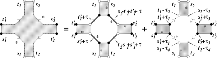
Figure 6: Diagrams representing the two contributions to the correlator ${\cal F}(t_{1},t_{1}^{\prime};t_{2},t_{2}^{\prime};s_{1},s_{1}^{\prime};s_{2},s_{2}^{\prime})$ (l.h.s.). The first diagram on the r.h.s. contains Gaussian contractions only; the shaded blocks in denote the kernel $D$. The second diagram on the r.h.s. contains one non-Gaussian contraction, which is in the center of the diagram; the shaded blocks represent factors of the form $(M+\partial_{\tau})D$, see equation (75) and figure 4d.

We used equations (72) and (71) to calculate time derivatives of the diffusons. Alternatively, using a partial integration, the function ${\cal F}$ can be expressed by equation (76) with

$$\Gamma=M-\tr R(t_{1}^{\prime}+\tau)R^{\dagger}(s_{1}^{\prime}+\tau)-\tr R(t_{2}-s_{1}+s_{1}^{\prime}+\tau)R^{\dagger}(s_{2}-t_{1}+t_{1}^{\prime}+\tau)$$

$$\mbox{}+\tr R(t_{1}^{\prime}+\tau)R^{\dagger}(s_{2}-t_{1}+t_{1}^{\prime}+\tau)R(t_{2}-s_{1}+s_{1}^{\prime}+\tau)R^{\dagger}(s_{1}^{\prime}+\tau)$$

$$\mbox{}-\delta(\tau)-\delta(\tau-t_{1}+t_{1}^{\prime}+s_{2}-s_{2}^{\prime}).$$ (78)

or with $\Gamma$ given by a convenient linear combination of equations (77) and (78) with coefficients $C_{1},C_{2}$ satisfying the condition $C_{1}+C_{2}=1$.

Finally, using equation (28) for $R$, the first term of equation (38) is obtained. The other contributions to equation (38) can be found after permutation of the channel indices and time-variables as indicated in figure 2.

References

References

• [1] Mehta M L 1991 Random Matrices (New York: Academic)
• [2] Mello P A 1995 Mesoscopic Quantum Physics ed E Akkermans, G Montambaux, et al. (Amsterdam: North-Holland) p 437
• [3] Guhr T, Müller-Groeling A, and Weidenmüller H A 1998 Phys. Rep. 299 189
• [4] Porter C E 1965 Statistical Theories of Spectra: Fluctuations (New York: Academic)
• [5] Brody T A, Flores J, French J B, Mello P A, Pandey A and Wong S S M 1981 Rev. Mod. Phys. 53 385
• [6] Bohigas O, Giannoni M J and Schmit C 1984 Phys. Rev. Lett. 52 1
• [7] Bohigas O 1991 Chaos and Quantum Physics ed M-J Giannoni, A Voros and J Zinn-Justin (Amsterdam: North-Holland) p 87
• [8] Kouwenhoven L P, Marcus C M, McEuen P L, Tarucha S, Westervelt R M and Wingreen N S 1997 Mesoscopic Electron Transport, NATO ASI Series E vol 345, ed L L Sohn, L P Kouwenhoven and G Schön (Dordrecht: Kluwer)
• [9] Alhassid Y 2000 Rev. Mod. Phys. 72 895
• [10] Efetov K B 1997 Supersymmetry in Disorder and Chaos (New York: Cambridge University Press)
• [11] Beenakker C W J 1997 Rev. Mod. Phys. 69 731
• [12] Verbaarschot J J M, Weidenmüller H A and Zirnbauer M R 1985 Phys. Rep. 129 367
• [13] Lewenkopf C H and Weidenmüller H A 1991 Ann. Phys. 212 53
• [14] Blümel R and Smilansky U 1988 Phys. Rev. Lett. 60 477
• [15] Blümel R and Smilansky U 1990 Phys. Rev. Lett. 64 241
• [16] Smilansky U 1991 Chaos and Quantum Physics ed M-J Giannoni, A Voros, and J Zinn-Justin (Amsterdam: North-Holland) p 371
• [17] Baranger H U and Mello P A 1994 Phys. Rev. Lett. 73 142.
• [18] Jalabert R A, Pichard J-L and Beenakker C W J 1994 Europhys. Lett. 27 255
• [19] Mello P A, Pereyra P and Seligman T H 1985 Ann. Phys. 161 254
• [20] Brouwer P W 1995 Phys. Rev. B 51 16878
• [21] Switkes M, Marcus C M, Campman K and Gossard A C 1999 Science 283 1905
• [22] Vavilov M G and Aleiner I L 1999 Phys. Rev. B 60 16311
• [23] Vavilov M G and Aleiner I L 2001 Phys. Rev. B 64 085115
• [24] Huibers A G, Folk J A, Patel S R, Marcus C M, Duruöz C I and Harris J S 1999 Phys. Rev. Lett. 83 5090
• [25] Wang X B and Kravtsov V E 2001 Phys. Rev. B 64 033313
• [26] Kravtsov V E 2001 Preprint cond-mat/0106241
• [27] Yudson V I, Kanzieper E and Kravtsov V E 2001 Phys. Rev. B 64 045310
• [28] Dyson F J and Mehta M L 1963 J. Math. Phys. 4 701
• [29] Büttiker M, Prêtre A and Thomas H 1993 Phys. Rev. Lett. 70 4114
• [30] Büttiker M 1993 J. Phys. Condens. Matter 5 9361;
• [31] Büttiker M, Thomas H and Prêtre A 1994 Z. Phys. B 94 133
• [32] Büttiker M and Christen T 1996 Quantum Transport in Semiconductor Submicron Structures, NATO ASI Ser. E vol 326 ed B Kramer (Dordrecht: Kluwer) p 263
• [33] Büttiker M 2000 J. Low Temp. Phys. 118 519
• [34] Shutenko T A, Aleiner I L, and Altshuler B L 2000 Phys. Rev. B 61 10366
• [35] Vavilov M G, Ambegaokar V, and Aleiner I L 2001 Phys. Rev. B 63 195313
• [36] Brouwer P W and Beenakker C W J 1996 J. Math. Phys 37 4904
• [37] Polianski M L, Vavilov M G and Brouwer P W 2002 Phys. Rev. B 65 245314
• [38] Jalabert R A, Baranger H U and Stone A D 1990 Phys. Rev. Lett. 65 2442
• [39] Stone A D 1995 Mesoscopic Quantum Physics ed E Akkermans, G Montambaux et al. (Amsterdam: North-Holland) p 327
• [40] Argaman N 1995 Phys. Rev. Lett. 75 2750
• [41] Vallejos R O and Lewenkopf C H 2001 J. Phys. A 34 2713
• [42] Samuel S 1980 J. Math. Phys. 21 2695
• [43] Mello P A 1990, J. Phys. A 23 4061
• [44] Efetov K B 1995 Phys. Rev. Lett. 74 2299
• [45] Frahm K 1995, Europhys. Lett. 30 457
• [46] Brouwer P W and Büttiker M 1997 Europhys. Lett. 37 441
• [47] Aleiner I L, Brouwer P W and Glazman L I 2002 Phys. Rep. 358 309
• [48] Brouwer P W and Beenakker C W J 1996 Phys. Rev. B 54 12705
• [49] Brouwer P W, Frahm K M and Beenakker C W J 1999 Waves in Random Media 9 91
• [50] Kottos T and Smilansky U 1997 Phys. Rev. Lett. 79 4794
• [51] Brouwer P W, Cremers J N H J and Halperin B I 2002 Phys. Rev. B 65 081302
• [52] Spivak B, Zhou F and Beal Monod M T 1995 Phys. Rev. B 51 13226
• [53] Brouwer P W 1998 Phys. Rev. B 58 10135
• [54] Zhou F, Spivak B and Altshuler B L 1999 Phys. Rev. Lett. 82 608
• [55] Frahm K and Pichard J-L 1995 J. Phys. (France) I 5 847
• [56] Adam S, Polianski M L, Waintal X and Brouwer P W 2002 Preprint cond-mat/0206377
• [57] Büttiker M 1990 Phys. Rev. Lett. 65 2901
• [58] Büttiker M 1992 Phys. Rev. B 45 3807
• [59] Büttiker M 1992 Phys. Rev. B 46 12485
• [60] Baranger H U and Mello P A 1995 Phys. Rev. B 51 4703
• [61] Aleiner I L and Larkin A I 1996 Phys. Rev. B 54 14423
• [62] Brouwer P W and Beenakker C W J 1997 Phys. Rev. B 55 4695.
• [63] Fal’ko V I and Khmelnitskii D E 1989 Zh. Eksp. Teor. Fiz 95 328 (Engl. Transl. 1989 Sov. Phys. JETP 68 186)
• [64] Blanter Y M and Büttiker M 2001 Phys. Rep. 336 1
• [65] Andreev A V and Kamenev A 2000 Phys. Rev. Lett. 85 1294
• [66] Levitov L S 2001 Preprint cond-mat/0103617
• [67] Andreev A V and Mishchenko E G 2001 Phys. Rev. B 64 233316
• [68] Makhlin Yu and Mirlin A D 2001 Phys. Rev. Lett. 87 276803
• [69] Moskalets M and Büttiker M 2002 Phys. Rev. B 66 035306
• [70] Nazarov Yu V 1995 Quantum Dynamics of Submicron Structures, NATO ASI Series vol 291 ed H A Cerdeira, B Kramer and G Schön (Dordrecht: Kluwer) p 687
• [71] Friedman W A and Mello P A 1985 Ann. Phys. 161 276