Hölder exponent spectra for human gait

Abstract

The stride interval time series in normal human gait is not strictly constant, but fluctuates from step to step in a complex manner. More precisely, it has been shown that the control process for human gait is a fractal random phenomenon, that is, one with a long-term memory. Herein we study the Hölder exponent spectra for the slow, normal and fast gaits of 10 young healthy men in both free and metronomically triggered conditions and establish that the stride interval time series is more complex than a monofractal phenomenon. A slightly multifractal and non-stationary time series under the three different gait conditions emerges.

]

I Introduction

In the past two decades we have witnessed an explosion in the biophysics and physiological literature with regard to the identification of phenomena having long-term memory and probability densities that extend far beyond the typical tail region of Gaussian distributions. One way these processes have been classified is as 1/f-phenomena, since their time series have spectra that are inverse power law in frequency or their probabilities are inverse power law. In either case the underlying structure is fractal, either in space, time or both [1]. Herein we are interested in demonstrating that human gait time series, see Fig. 1, is more than monofractal. By estimating the Hölder exponents and their spectra using wavelet transform [2], we show that the stride interval time series is weakly multifractal; the time series is sometimes non-stationary and its fractal variability changes in different gait mode regimes.

The gait data we study are in public domain archives Physionet [3], which we downloaded. The data sets are the stride interval time series for 10 healthy young men walking at slow, normal and fast paces in both free and metronomically triggered conditions for a period of one hour in the former and 30 minutes in the latter cases, respectively. These data were originally collected and used by Hausdorff et al. [4] to determine the dependence of the fractal dimension of the time series on changes of the average rate of walking. Given their positive results it is not a surprise that the gait time series is not monofractal, but is multifractal, with a dependence on the average rate of walking.

In Sec. 2 we give a short introduction to the phenomenon of locomotion, the traditional methods for modeling using the Central Pattern Generator (CPG), and review the data processing used to establish the fractal behavior of stride time interval time series. Sec. 3 reviews various ways to estimate the Hölder exponents and singularity spectra. In particular, the relationship between the singularity spectrum and the probability density for the realization of a particular Hölder exponent is discussed in the context of modeling the motocontrol system. The results of the data processing are presented in Sec. 4. Finally, in Sec. 5 we discuss our results and compare them with those of Hausdorff et al. [4].

II Complexity of locomotion

Walking consists of a sequence of steps and the corresponding time series consists of the time intervals for these steps. These steps may be partitioned into two phases: a stance phase and a swing phase. The stance phase is initiated when a foot strikes the ground and ends when it is lifted. The swing phase is initiated when the foot is lifted and ends when it strikes the ground again. The time to complete each phase varies with the stepping speed. A stride interval is the length of time from the start of one stance phase to the start of the next stance phase. It is the variability in the time series made from these stride intervals that we address in this paper.

Traditionally the legged locomotion of animals is understood through the use of a Central Pattern Generator (CPG), an intraspinal network of neurons capable of producing a syncopated output [5]. The implicit assumption in such an interpretation is that a given limb moves in direct proportion to the voltage generated in a specific part of the CPG. Experiments establishing the existence of a CPG have been done on animals with spinal cord transections. It has been shown that such animals are capable of walking under certain circumstances. Walking, for example, in a mesencephalic cat, a cat with its brain stem sectioned rostral to the superior colliculus, is very close to normal, on a flat, horizontal surface, when a section of the midbrain is electrically stimulated. Stepping continues as long as a train of electrical pulses is used to drive the stepping. This is not a simple linear response process, however, since the frequency of the stepping increases in proportion to the amplitude of the stimulation, whereas changing the frequency of the driver has little effect of the walking [6].

As Collins and Richmond [5] point out, in spite of the studies establishing the existence of a CPG in the central nervous system of quadrupeds, such direct evidence does not exist for a vertebrate CPG for legged locomotion. Consequently, these and other authors have turned to the construction of models, based on the coupling of nonlinear oscillators, to establish that the mathematical models are sufficiently robust to mimic the locomotion characteristics observed in the movements of segmented bipeds [7], as well as in quadrupeds [8]. These characteristics, such as the switching among multiple gait patterns, is shown to not depend on the detailed dynamics of the constituent nonlinear oscillators, nor on their inter-oscillator coupling strengths [5].

It has been known for over a century that there is a variation in the stride interval of humans during walking of approximately 3-4% [9]. This random variability is so small that the biomechanical community has historically considered these fluctuations to be an uncorrelated random process. In practice this means that the fluctuations in gait were thought not to contain any useful information about the underlying motocontrol process. On the other hand, Hausdorff et al. [4, 10] demonstrated that stride-interval time series exhibit long-time correlations, and suggested that the phenomenon of walking is a self-similar, fractal, activity. Subsequent studies by West and Griffin [11, 12, 13] support these conclusions using a completely different experimental protocol for generating the stride-interval time series data and very different methods of analysis. The existence of fractal time series suggests that the nonlinear oscillators needed to model locomotion operates in the unstable, that is, in the chaotic regime.

A stochastic version of a CPG was developed by Hausdorff et al. [4] to capture the fractal properties of the inter-stride interval time series. This stochastic model was later extended by Ashkenazy et al. [14] to describe the changing of gait dynamics as we develop from being a child to being an adult. The model is essentially a random walk on a chain, where each node of the chain is a neural center of the kind discussed above, and with a different frequency. This random walk is found to generate a multifractal rather than a monofractal process, with a width that depends parametrically on the range of the walker’s step size. Ashkenazy et al. [14] focused on explaining the changes in the gait time series during maturation, using the stochastic CPG model. In addition, they applied the multifractal formalism to the computer-generated time series, to obtain the singularity spectrum, but they did not obtain such a spectrum using the experimental inter-stride interval time series. A related model, using a fractional Langevin equation, was proposed by West et al. [15] in which the multifractality of the signal is interpreted as a fluctuating scaling parameter.

Herein we use stride interval data to further refine the stochastic analysis for human gait by estimating the local Hölder exponents of the stride interval that measure the local fractality of a time series and the properties of their distributions.

III Hölder exponent distribution

In this section we give a short review of the analysis method we apply to human gait data. In The Fractal Geometry of Nature [16], Mandelbrot showed that many natural phenomena are described by self-affine, correlated, time series. The scaling properties of such fractal noise, Fractional Gaussian Noises (FGN), are characterized by an exponent that Mandelbrot called $H$ in honor of Hurst. If $X(t)$ is a fractal process with Hurst exponent $H$ and $c$ is a constant, then $X\left(t\right)=X(ct)/c^{H}$ is another fractal process with the same statistics. FGN is defined by a spectrum satisfying the power law

$$P(f)\propto f^{-\beta}~{},$$ (1)

where $f$ is the frequency, the exponent $\beta=(2H-1)$ and $H$ is the Hurst exponent. The self-affine property expressed by (1) and the relation between $\beta$ and $H$ are theoretically valid only for an infinitely long monofractal noise.

Fig. 2 shows a computer generated realization of FGN with Hurst exponent $H=1$, also known as $1/f$ noise or pink noise. This type of noise is important because it is a kind of threshold between the persistent-stationary noise ($0.5<H<1$ or, assuming the asymptotic relation between the two parameters, $0<\beta<1$) and the non-stationary noise ($\beta>1$). Note that the common term random or white noise is characterized by $\beta=0$ or $H=0.5$ whereas the random walk or Brownian motion is characterized by $\beta=2$. The noise characterized by $0<H<0.5$ is called anti-persistent, whereas the noise characterized by $0.5<H<1$ is called persistent [16]. In the same way, we may call anti-persistent the walk given by the fluctuations characterized by $1<\beta<2$ and persistent the walk given by the fluctuations characterized by $2<\beta<3$. The fluctuations characterized by an exponent $1<\beta<3$ we call walks because they may be obtained by integrating fractal noises characterized by Hurst exponents in the interval $0<H<1$.

In our numerical example, we use pink noise because the gait data, as shown in the next section, are characterized by properties that range from a strong persistent-stationary noise to a weak non-stationary walk. As seen in Fig. 2, a fractal noise is characterized by trends and discontinuities that give a particular geometric shape to the signal. The rapid changes in the time series are called singularities of the signal and their strength is measured by a Hölder exponent [2]. Given a function $f(x)$ with a singularity at $x_{0}$, the Hölder exponent $h(x_{0})$ at such a point is defined as the supremum of all exponents $h$ that fulfills the condition:

$$|f(x)-P_{n}(x-x_{0})|\leq C|x-x_{0}|^{h}~{},$$ (2)

where $P_{n}(x-x_{0})$ is a polynomial of degree $n<h$. The relation between the Hölder and Hurst exponents in the continuum limit is $h=H-1$.

A Continuous wavelet transform.

The Hölder exponent of a singularity can be evaluated by using the wavelet transform. Wavelet analysis [17, 18, 19] has become a powerful method to analyze time series. Wavelet transforms makes use of scaling functions that have the property of being localized in both time and frequency. A scaling coefficient $s$ characterizes and measures the width of a wavelet. Given a signal $f(x)$, the continuous wavelet transform (CWT) of $f(x)$ is defined by

$$W_{s,x_{0}}(f)=\int\limits_{-\infty}^{\infty}\frac{1}{s}~{}\psi\left(\frac{x-x_{0}}{s}\right)~{}f(x)~{}dx~{},$$ (3)

where the kernel $\psi(u)$ is the wavelet filter centered at the origin, $u=0$, with unit width, $s=1$.

The wavelet transform can be used to determine the Hölder exponent of a singularity because the wavelet kernel $\psi(u)$ can be chosen in such a way as to be orthogonal to polynomials up to degree $n$, that is, such that the following properties are fulfilled

$$\int\limits_{-\infty}^{+\infty}\frac{1}{s}~{}\psi\left(\frac{x-x_{0}}{s}\right)~{}x^{m}~{}dx=0~{}~{}~{}\forall m,~{}0\leq m\leq n~{}.$$ (4)

In fact, if (4) holds true, it is easy to prove that if the function $f(x)$ fulfils condition (2), its wavelet trasform at $x=x_{0}$ is given by

$$W_{s,x_{0}}(f)=C|s|^{h(x_{0})}\int\limits_{-\infty}^{+\infty}|u|^{h(x_{0})}~{}\psi(u)~{}du\propto|s|^{h(x_{0})}~{},$$ (5)

where $u=(x-x_{0})/s$. Therefore, at least theoretically, the Hölder exponent of a singularity can be evaluated as the scaling exponent of the wavelet transform coefficient, $W_{s,x_{0}}(f)$, for $s\to 0$.

In this paper we make use of the Mexican Hat wavelet, the second derivative of a Gaussian, and which is defined by

$$\psi(u)=(1-u^{2})\exp(-u^{2}/2)~{}.$$ (6)

The Mexican Hat wavelet integrates to zero polynomial biases up to degree $n=1$. Finally, due to the exponential convergence to zero of Eq. (6) for large $|u|$, we may assume that the Mexican Hat wavelet explores a window size approximately 10 times the scale $s$.

B Maxima lines and multifractal formalism.

Even if Eq. (5) can be evaluated for any position $x_{0}$, we are interested only in the cusp singularities of the time series. Mallat et al. [18, 20, 21] show that the Hölder exponent of these singularities can be evaluated by studying the scaling exponent $h(x_{0})$ along the so-called maxima line that converges towards the singularity. The maxima lines are defined by the extremes of the wavelet transform coefficients (3) at each wavelet scale $s$.

Fig. 3 shows the wavelet transform modulus maxima (WTMM) line tree of the fractal noise of Fig. 2. Fig. 3 shows that, in a complex process, the singularities become less and less isolated as the scaling coefficient $s$ increases. This means that it is not possible, in general, to use Eq. (5) to evaluate the Hölder exponent of a singularity because the maxima line of a singularity will be deformed by its neighboring singularities. However, Arneodo et. al. [22, 23] proved that WTMM can be used to define a multifractal-like formalism that gives the stochastic properties of the singularities of a fractal or multifractal noise.

The idea is to evaluate the mass exponent $\tau(q)$ of the moment $q$ from the partition function $Z(s,q)$ assuming that

$$Z(s,q)=\sum_{\Omega(s)}|W_{s,x_{0}}(f)|^{q}\propto s^{\tau(q)}~{},$$ (7)

where the sum is over the set $\Omega(s)$ of all maxima at the scale $s$. The entire distribution of Hölder exponents can be determined because negative $q$ stress weak singularities whereas positive $q$ stress strong singularities. Finally, by using the Legendre transformation it is possible to define the spectrum of the singularities $D(h)$ by

$${h(q)=d\tau(q)/dq\atop D[h(q)]=qh(q)-\tau(q)~{}.}$$ (8)

Eq. (8) gives a global average of the strength of the singularities of the time series and it has been recently used to determine the multifractal nature of many signals, for example, that for human heartbeats [24].

C Approximate estimation of local Hölder exponents and their probability distribution

The spectrum of the singularities $D(h)$ defined by Eqs. (8) presents some problems of stability when applied to observational data. In fact, the spectrum can be corrupted by the divergences of negative moments [18, 23, 25] or by the outliers, that is, the end points of the sample singularities [2]. Different methods have been suggested to remove the divergences due to the negative moments of the multifractal partition function, for example, by chaining the wavelet maxima across scales [18] or, more efficiently, by bounding the Hölder exponent of the maxima line by using the slope wavelet [25]. The corruption of the singularity spectrum due to the outliers is more difficult to deal with.

Struzik [2] suggested an alternative method that has the ability to determine an approximate value of local singularity strength. The spectrum may then be evaluated from these approximate values. The idea is to estimate the mean Hölder exponent $\overline{h}$ as a linear fit of the following equation

$$\log[M(s)]=\overline{h}~{}\log(s)+C~{},$$ (9)

where the function $M(s)$ is obtained via the partition function, Eq. (7),

$$M(s)=\sqrt{\frac{Z(s,2)}{Z(s,0)}}~{}.$$ (10)

Eqs. (9) and (10) allow us to consider the mean Hölder exponent $\overline{h}$ to be the local version of the Hurst exponent $H$ [16]. More precisely, for a monofractal noise with Hurst exponent $H$, we have $\overline{h}=H-1$ because the Hurst exponent is evaluated by integrating the noise [16, 26]. Here again the equality is only rigorously true for an infinitely long monofractal noise data set. The approximate local Hölder exponent $\hat{h}(x_{0},s)$ at the singularity $x_{0}$ can now be evaluated as the slope

$$\hat{h}(x_{0},s)=\frac{\log(|W_{s,x_{0}}(f)|)-(\overline{h}~{}\log(s)+C)}{\log(s)-\log(s_{N})}~{},$$ (11)

where $s_{N}$ is the length of the entire wavelet maxima line tree, that is, the maximum available scale that coincides with the sample length $s_{N}=N$, and $x_{0}$ belongs to the set $\Omega(s)$ of all wavelet maxima at the scale $s$ that assume the value $W_{s,x_{0}}(f)$.

Fig. 4 gives a graphical view of how the local Hölder exponent $\hat{h}(x_{0},s)$ are evaluated. We plot $\log[|W_{s,x_{0}}(f)|]$ against $\log(s)$ for all wavelet maxima at many scales. The black crosses are the mean Hölder exponents evaluated by using Eq. (9) and are fitted in the interval [0,3] that corresponds to the scales $1\leq s\leq 20$, that yields $\overline{h}=-0.004\pm 0.008$ and $C=1.00\pm 0.02$. The intersection point on the right of the fitting line is the root of the wavelet line tree and corresponds to $\log(s_{N})=\log(5000)=8.52$. Finally, the local Hölder exponent $\hat{h}(x_{0},s)$ are evaluated as the slope of the straight line that joins the root of the wavelet line tree to the value of the wavelet coefficient $\log[|W_{s,x_{0}}(f)|]$ at each singularity at the scale $s$. The slope of the two straight lines shown in the figure represent the maximum and minimum value of $h$.

Fig. 5 shows the Hölder exponents for the FGN plotted against the position in the time series. Finally, Fig. 6 shows the histogram of Hölder exponents obtained using a computer-generated data set with a Hurst exponent $H=1$. The probability distribution, that gives the spectra of the Hölder exponents, is estimated with a histogram whose number of bins is chosen, for stochastic stability, equal to the square root of the number singularities at the scale analyzed. In our example we use the smallest available scale, that is, $s=1$. Note that to obtain a shape similar to that usually seen for a multifractal singularity spectrum, the probability distribution $p(h)$ should be graphed on a log-linear graph paper. In fact, according to the thermodynamic picture of multifractal behavior developed in Ref. [27], the number $M(h)$ of boxes of size $\varepsilon$ with a Hölder exponent $h$ has the scaling behavior

$$M(h)\sim\varepsilon^{-D(h)}~{},$$ (12)

where $D(h)$ is the singularity spectrum. Introducing $V=-\log(\varepsilon)$, the probability that the Hölder exponent in the interval $(h,h+dh)$ is

$$p(h)=\frac{\exp[V~{}D(h)]}{Z}~{},$$ (13)

where $Z$ is the partition function. Eq. (13) suggests that the singularity spectrum $D(h)$ can be interpreted as the entropy density of the escort distribution $S(h)=\log[p(h)]$ in the limit $\varepsilon\to 0$ limit, that is,

$$\lim_{V\to\infty}\frac{S(h)}{V}=D(h)~{}.$$ (14)

D Fractal or multifractal?

Fig. 6 shows the histogram of Hölder exponents for the artificial fractal noise of Fig. 2 produced with the Hurst exponent $H=1$. Actually, we plot the probability density $p(h)$ against $h$, that is, the probability to find an Hölder exponent in a bin of size $\varepsilon$ divided by the size $\varepsilon$. The size $\varepsilon$ is determined by dividing the range between the maximum and the minimum of the Hölder exponents by the square root of the number af all evaluated Hölder exponents. The probability distribution of Hölder exponents of our computer generated noise has as its mean $\overline{h}=-0.004\pm 0.008$ that is consistent with the value $h=H-1=0$ that characterizes pink noise. By fitting the histogram with the normalized Gaussian

$$g(h)=\frac{1}{\sqrt{2\pi}~{}\sigma}~{}\exp{\left[-\frac{(h-h_{0})^{2}}{2~{}\sigma^{2}}\right]}$$ (15)

it is possible to evaluate the width of the distribution $\sigma$. Note that usually $h_{0}$ may be slightly larger than $\overline{h}$ because the distribution of the Hölder exponents may present a slightly positive skewness, so, in this computer generated noise, we measure $h_{0}=0.007\pm 0.001$ and $\sigma=0.052\pm 0.002$. The width $\sigma$ is not zero, as would be expected for an infinitely long computer-generated monofractal noise. This non-zero $\sigma$ may be mistaken for an indicator of multifractal behavior. However, the non-vanishing value of $\sigma$ for our computer-generated noise is due to the fact that a monofractal noise has some variability of the local Hölder exponents and to the finite size $N=5000$ of the sample. The width $\sigma$ of the histogram is expected to converge to zero as $N\to\infty$.

The problem is to distinguish fractal noise from multifractal noise. The idea is that a multifractal noise is characterized by a probability distribution of Hölder exponents wider than that of a correspondent monofractal noise. Therefore, with the help of Eq. (15) we suggest the following procedure for studying the multifractality of a time series of finite length $N$: (i) we evaluate the mean Hölder exponent $\overline{h}$ and the width $\sigma$ of the histogram that estimates the probability distribution of the Hölder exponents of such datasets by using the Gaussian (15); (ii) we generate many artificial datasets of fractal noise of finite length $N$ and with a Hurst coefficient $H=\overline{h}+1$ and study the distribution of the monofractal widths $\sigma_{F}$; (iii) finally, if $\sigma$ is larger than $\sigma_{F}$ and this is statistically significant, we conclude that the original time series is multifractal.

IV Human gait analysis

We now present the analysis of the human gait of 10 persons in the three different conditions of slow, normal and fast walking for a period of approximately one hour (unconstrained walking) and 30 minutes (metronomically constrained walking) in each condition. Figures 1 and 7 show two typical sets of data for particular walkers under the three conditions.

Participants in the study had no history of any neuromuscular, respiratory or cardiovascular disorders. They were not taking any medications and had a mean age of 21.7 years (range: 18-29 years); height $1.77\pm 0.08$ meters and mean weight $71.8\pm 10.7$ kg. All subjects provided informed written consent. Subjects walked continuously on level ground around an obstacle-free, long (either 225 or 400 meters), approximately oval path and the stride interval was measured using ultra-thin, force sensitive switches taped inside one shoe. For the metronomically constrained walking, the individuals were told only once, at the beginning of their walk, to synchronize their steps with the metronome. More details regarding the collection of data can be found in Physionet [3] from where the data were downloaded and in Ref. [4].

A Free-pace walking

Table 1 records the basic properties of the 30 gait datasets at the unconstrained walking condition. We tabulate the number of strides ($N$), mean stride interval ($T$) and standard deviation of the stride interval for the three gait conditions for each of the ten walkers. The data condensed in Table 1 show a large variation in parameter values from person to person. The mean value of the stride interval in the case of slow gait is $T=1.324$ sec., in the case of normal gait is $T=1.117$ sec., and in the case of fast gait is $T=1.001$ sec.. Person number 8 has the slowest walk with $T=1.790$ sec. and the standard deviation is the highest with $St~{}Dev=0.15$ sec. Persons 1, 2 and 3 do not present large differences between slow and normal gait if we focus on their mean stride interval time.

Table 2 shows the mean Hölder exponent $\overline{h}$ determined using Eq. (9) for the 30 gait datasets. The fit is done on the scale interval $1\leq s\leq 20$ that allows us to explore windows up to approximately 200 strides. Table 3 records the basic properties of the Hölder exponent distribution, explained in the previous section, for the 30 gait datasets. The mean $h_{0}$ and the width of the distribution $\sigma$ are estimated by fitting the histogram with the normalized Gaussian of Eq. (15) as done in Fig. 6 for computer generated FGN. The error of measure on the mean value $h_{0}$ is estimated to be $\pm 0.0025$ on average, whereas the error on the width $\sigma$ is $\pm 0.002$ on average.

Table 3 also records the width $\sigma_{F}$ of the distribution of Hölder exponents for computer-generated datasets of monofractal noise with $H=1+\overline{h}$ of $N$ elements in correspondence of each of the 30 gait datasets. The values $\sigma_{F}$ are evaluated by averaging 20 computer simulations. The table shows that, even by considering the error of measure of $\pm 0.002$, the width of the Hölder exponent distribution $\sigma$ is almost always slightly larger than the width $\sigma_{F}$ for a corresponding monofractal noise of Hurst exponent $H=\overline{h}+1$ of equal size sample $N$. On average, we get that for slow gait $\sigma$ is $8.3\%$ larger than $\sigma_{F}$, for the normal gait $\sigma$ is $4.7\%$ larger than $\sigma_{F}$ and, finally, for the fast gait $\sigma$ is $4.9\%$ larger than the correspondent $\sigma_{F}$. In particular, for the slow gait of person number 8, see Figs. 7 and 8B, $\sigma$ is $40\%$ larger than $\sigma_{F}$.

Table 4 reports the results of the Student’s t-test in the case of paired samples [28] between the histogram widths $\sigma$ and $\sigma_{F}$ for the 10 walkers in the three gait conditions recorded in Table 3. We use the paired samples algorithm because the values of the widths $\sigma$ and $\sigma_{F}$ depend on the size of the sample $N$ and the Hurst exponent $H$. So, we have to imagine that the variance in both samples may be due to effects that are point-by-point identical in the two samples. The value $t$ is the Student’s t value and $prob$ is the probability that the two sets of data for each walking condition have the same mean. Figs. 8A and 8B show the probability density function of the Hölder exponents for walker number 5 (Fig. 8A) and walker number 8 (Fig. 8B). Finally, Fig. 9 shows the global distribution of the Hölder exponents for the three different gaits whose characteristics are condensed in Table 5. Three symbols –star, triangle and circle– indicate the three gaits –slow, normal and fast–. The distributions are fitted by normalized Gaussian functions, Eq. (15).

Fig. 9 and Table 5 show the global properties of the distributions of all Hölder exponents for the three different gait modes that have been measured for the ten persons. By increasing the average rate of walking from slow to normal the mean of the Gaussian, $h_{0}$, on average decreases, whereas increasing the average rate of walking from normal to fast, $h_{0}$ increases on average. There is also an increasing of the width of the distribution $\sigma$ by moving from the normal to the slow or fast gait mode. This last result indicates that normal human gait is more standard than the other two types of gait in the sense that many persons, when asked to walk normally, present a similar distribution of Hölder exponents for the stride interval time series. Moreover, we note a large width of the distribution of the Hölder exponents in the case of slow gait. This means that there is a large variability in the distribution of Hölder exponents for slow human gait, that is, a large variability of the fractal properties of the stride interval time series among the persons who are asked to walk slowly.

B Metronomically-pace walking

Figs. 10 show two of the ten individuals of metronomically constrained walking for the three gait conditions; slow, normal and fast walking. The total period for each dataset is approximately 30 minutes. Table 6 records the basic properties of the 30 gait datasets. The mean values of the stride interval is compatible with those obtained for the unconstrained walking: in the case of slow gait $T=1.356$ sec.; in the case of normal gait $T=1.116$ sec.; and in the case of fast gait $T=1.003$ sec.. However, by comparing Tables 1 and 6 as well as Figs. 1, 7 and 10, we notice that the constrained walking presents a smaller standard deviation and much less variability of the strength of the local biases of the stride interval time series. This can be understood as an effect due to the unvaryingly regular artificial rhythm that constrains the walking.

Table 7 shows the mean Hölder exponent $\overline{h}$ determined using Eq. (9) for the 30 gait datasets. The fit is done on the scale interval $1\leq s\leq 10$ that allows us to explore windows up to approximately 100 strides. We use a scale interval up to $s=10$ because the fewer number of data points (almost one half of the previous case) makes the statistics poorer at higher scales and because, here, we study the differences that occurs among the three gait conditions at the shorter scale. Figs. 11A and 11B show the histograms of the Hölder exponents for walker number 3 (Fig. 11A), who can be considered to be typical of the ten walkers, and walker number 5 (Fig. 11B) characterized by a strong antipersistent behavior of the stride interval time series. Finally, Fig. 12 shows the global distribution of the Hölder exponents as results from the study of the 30 datasets for the three different gait modes. The figure shows wide spreading of the global distribution of Hölder exponents, a fact that suggests a large variability of situations from persistent to antipersistent conditions.

Table 8 reports the values $h_{0}$ and $\sigma$ of the normalized Gaussian functions, Eq. (15), that fit the histograms of the Hölder exponent probability density distribution. The values $\sigma_{F}$ are the estimated width of the Hölder exponent probability density distribution of the computer-generated monofractal noise with Hurst exponent $H=1+\overline{h}$ and of $N$ elements. Finally, Table 9 records the Student’s t-test is the case of paired samples between the histogram widths $\sigma$ and $\sigma_{F}$ for the 10 walkers in the three gait conditions. The value $t$ is the Student’s t value and $prob$ is the probability that the two sets of data for each walking condition have the same mean. Table 8 and the Student’s t-test shows that the widths $\sigma$ are usually larger than the correspondent $\sigma_{F}$ and this increase is statistically significant.

V Discussion and conclusion

Hausdorff et al. [4] established that during the metronomically-paced walking, the long-range correlations of up to 1000 strides detected in the three modes of free walking disappear and variations in the stride interval are anti-correlated. These results are confirmed by the present analysis. However, the study of the distribution of the Hölder exponents allows for an even richer interpretation of the scaling behavior of the inter-stride interval time series. The time series is not monofractal, as was suggested by earlier analysis [10, 13], but is here determined to be weakly multifractal. The multifractality does not strictly invalidate the interpretation of scaling behavior, that being, that the statistical correlations in the stride interval fluctuations over thousands of strides decay in a scale-invariant manner. But it does suggest that the scale-invariant decay of the correlations is more complicated than was previously believed.

The average Hölder exponent, or equivalently, the fractal dimension, is determined to be dependent on the average rate at which an individual walks, but not monotonically dependent. The fractal dimension for the fast gait lies between those for the slow and normal gaits, in the case of unconstrained walking. The ordering of the fractal dimension for the three modes of walking is not so evident for the metronomically constrained gait.

We note that in the case of unconstrained walking the standard deviation in the case of slow gait is usually larger, almost double, that of the fast and slow gait cases. One possible explanation of this larger variance is that the stride interval for slow gait may be characterized by a non-stationary change in the mean stride interval during walking, what Hausdorff et al. [4] refer to as loss of concentration. This non-stationarity is seen to be the case in Fig. 1 and more specifically in Fig. 7, for one individual, but this behavior is typical of all the walkers. It is also worth pointing out that the standard deviation of the stride interval fluctuations for the slow gait increases as the mean stride interval decreases. This suggests that the more slowly a person walks, the more difficult it is for that person to keep his/her gait regular.

The results condensed in Tables 2 and 3, and in Figs. 8 and 9 show a great deal of information about the fractal properties of human gait. Note that the mean Hölder exponent $\overline{h}$ is usually slightly smaller than the center of the Gaussian fitting distribution $h_{0}$ because the Hölder exponent distributions present a slight positive skewness. All distributions of Hölder exponents are centered very close to the value $h=0$ that characterizes pink noise. Normal gait always presents a negative mean Hölder exponent $\overline{h}$ but larger than $h=-0.2$. This fact indicates that the stride interval time series for normal gait is strongly persistent and stationary, characterized by long-range, fractal correlations.

Fast gait presents properties similar to those of the normal gait, but usually with a mean Hölder exponent slightly larger and closer to the threshold $h=0$. The fact that fast gait almost always presents a negative mean Hölder exponent $\overline{h}$ means that the stride interval time for fast gait can usually be considered to be strongly persistent noise that, and as in the previous case, is characterized by strong long-range, fractal correlations. By contrast, at least for two people (persons number 1 and 2), the threshold $h=0$ of the pink noise is surpassed. This means that in these two cases the stride interval time fluctuations are slightly non-stationary. This last result emphasizes the range of dynamics of normal healthy gait.

On the contrary, the stride interval time series for slow gait, usually presents a mean Hölder exponent $\overline{h}$ slightly larger than the pink noise threshold $h=0$. This shift in the peak of the distribution to more positive Holder exponents implies that the slow gait is usually characterized by non-stationary fluctuations of the stride interval time series. Therefore, the slow gait regime could be considered a strongly anti-persistent and non-stationary walk rather than a strongly persistent noise. Perhaps, this slight non-stationarity in the slow gait is related to the fact that, contrary to the normal and, in part, the fast gait, walking slowly may require more concentration and a person asked to walk slowly may unconsciously lose this concentration and change the way of walking as he or she feels more comfortable.

The comparison between the probability density widths $\sigma$ for the gait data and $\sigma_{F}$ for the correspondent monofractal noise, that are recorded in the Tables 3 and 4, supports the conclusion that human gait may be characterized on average by a form of multifractality. In fact, the slowest mode of walking has the most variability as measured by the relative width $\sigma/\sigma_{F}$. The fastest mode of walking is characterized by a relative width compatible to or slightly larger than that of the normal mode.

The metronomically constrained walking datasets presents more complex behavior than does the freely walking data. The values of the mean Hölder exponents $\overline{h}$ recorded in Table 7 and Fig. 12 show that the walking loses the strong persistence of the unconstrained gait and becomes more random ($\overline{h}\approx-0.5$) or antipersistent ($\overline{h}<-0.5$). However, the normal gait still presents persistent behavior for many individuals. This indicates that spontaneous walking is less influenced by external constraints than either the fast of slow walking conditions. We stress the fact that for constrained gait our analysis concerns windows of width up to 100 strides. The fast gait becomes more random on average. This may indicate that a synchronization of the walking is easier in the fast regime. The slow gait shows a wider spectrum of situations from persistent to antipersistent noise, $-0.9<\overline{h}<-0.1$ indicating that synchronization of the walking is more difficult for some people in the slow regime.

We notice that at least one person, walker number 5, presents a strong antipersistency, $\overline{h}<-0.9$, for each of the three gait conditions. This may indicate that this person, in trying to synchronize his walking to the frequency of the clock, is unable to find a standard condition at all three gait modes. Consequently, the walker continuously shifts his stride interval up and down in the vicinity of an average, giving rise to a strong antipersistent signal, see also Fig. 11B. Paradoxically, the antipersistence of the signal is strongest at the normal gait. This effect may be a consequence of normal gait being free from the supraspinal influences of the metronome. This individual finds it necessary to continuously readjust his walking to maintain synchrony with the metronome.

It is well known to everyone that has taken military basic training that there are some individuals who cannot march in cadence. Individual 5 seems to suffer from this particular malady, but this interpretation requires additional research.

Finally, Tables 8 and 9 allow the comparison between the probability density widths $\sigma$ for the gait data and $\sigma_{F}$ for the correspondent monofractal noise. The width $\sigma$ are often larger than the correspondent $\sigma_{F}$ for all three conditions and the Student’s t-test allows us to conclude that this difference is statistically significant. This supports the conclusion that the human gait is characterized on average by a form of multifractality for the metronomically constrained walking. Also in this case, the fast and the slow gait are likely to be more multifractal than normal gait.

We noted earlier that there are a number of mathematical versions of the Central Patten Generators (CPGs) used to model the groups of neurons producing the rhythmic signals that produce locomotion in animals and possibly in humans as well. Here we note that certain coupled nonlinear oscillator networks have trajectories that lie on strange attractors. In one such case the time series resulting from such solutions have been shown to be multifractal, which is to say, a singularity spectrum was calculated from the time series [29]. The properties of the solution to such a nonlinear dynamical system appears to be consistent with the processing results obtained herein for gait. For example, Nakamura [29] showed that the singularity spectrum has multiple scaling regions (peaks in the singularity spectrum) dependent on certain parameter values in the dynamical equations. Of course it is necessary to provide a physiological interpretation of the parameters in this nonlinear oscillator before making any claims as to applicability as a CPG model. We are presently exploring that possibility.

——–
Acknowledgment:
N.S. thanks the Army Research Office for support under grant DAAG5598D0002 and L.G. thanks the National Research Center Fellowship.

		Slow			Norm			Fast
walker	N	$T$	$St~{}Dev$	N	$T$	$St~{}Dev$	N	$T$	$St~{}Dev$
1	3304	1.167	0.03	3371	1.037	0.02	3595	1.006	0.02
2	3347	1.063	0.02	3357	0.964	0.02	3822	0.925	0.02
3	3257	1.088	0.02	3391	1.078	0.02	3517	0.979	0.01
4	2625	1.372	0.05	3126	1.124	0.02	3534	1.008	0.02
5	2496	1.461	0.05	3362	1.106	0.02	3819	0.948	0.03
6	2844	1.273	0.04	3297	1.108	0.02	3451	1.008	0.02
7	2717	1.338	0.06	2976	1.149	0.02	3447	1.058	0.02
8	2040	1.790	0.15	2902	1.183	0.02	3720	0.967	0.01
9	2764	1.315	0.02	3054	1.179	0.02	3447	1.042	0.01
10	2547	1.373	0.04	2977	1.242	0.02	3262	1.070	0.02
Ave.	2794	1.324	0.05	3181	1.117	0.02	3561	1.001	0.02

TABLE I.: Number of strides (N), mean stride interval (T) and standard deviation of the stride interval for the ten walkers. Each person walks for approximately one hour in each of three different modes: slow, normal and fast.

	Slow	Norm	Fast
walker	$\overline{h}$	$\overline{h}$	$\overline{h}$
1	$-0.013\pm 0.011$	$-0.068\pm 0.015$	$0.030\pm 0.007$
2	$-0.163\pm 0.008$	$-0.114\pm 0.012$	$0.027\pm 0.021$
3	$0.030\pm 0.018$	$-0.093\pm 0.011$	$-0.099\pm 0.018$
4	$0.087\pm 0.016$	$-0.117\pm 0.014$	$-0.077\pm 0.012$
5	$0.101\pm 0.013$	$-0.132\pm 0.012$	$-0.020\pm 0.009$
6	$0.090\pm 0.017$	$-0.081\pm 0.018$	$-0.134\pm 0.011$
7	$0.172\pm 0.032$	$-0.096\pm 0.016$	$-0.044\pm 0.010$
8	$0.034\pm 0.017$	$0.002\pm 0.015$	$-0.031\pm 0.019$
9	$0.003\pm 0.017$	$-0.085\pm 0.017$	$-0.114\pm 0.011$
10	$-0.056\pm 0.014$	$-0.188\pm 0.008$	$-0.027\pm 0.010$
Ave.	$0.028\pm 0.089$	$-0.097\pm 0.049$	$-0.049\pm 0.056$

TABLE II.: Mean Hölder exponent $\overline{h}$ given by Eq. (9) for the 30 gait datasets. The fit is done on the scale interval $1\leq s\leq 20$. The exponent $\overline{h}$ is related to the Hurst exponent $H$ via the relation $\overline{h}=H-1$.

		Slow			Norm			Fast
walker	$h_{0}$	$\sigma$	$\sigma_{F}$	$h_{0}$	$\sigma$	$\sigma_{F}$	$h_{0}$	$\sigma$	$\sigma_{F}$
1	-0.009	0.059	0.056	-0.063	0.062	0.055	0.041	0.059	0.055
2	-0.154	0.057	0.056	-0.110	0.053	0.055	0.019	0.060	0.054
3	0.026	0.059	0.056	-0.090	0.056	0.055	-0.095	0.061	0.055
4	0.090	0.058	0.056	-0.105	0.056	0.056	-0.072	0.054	0.055
5	0.105	0.060	0.057	-0.125	0.063	0.055	-0.012	0.056	0.054
6	0.088	0.060	0.056	-0.083	0.059	0.056	-0.128	0.059	0.055
7	0.161	0.061	0.056	-0.089	0.060	0.056	-0.035	0.057	0.055
8	0.075	0.081	0.058	-0.000	0.058	0.056	-0.040	0.055	0.054
9	-0.002	0.052	0.056	-0.090	0.057	0.056	-0.114	0.054	0.055
10	-0.031	0.064	0.057	-0.165	0.058	0.056	-0.011	0.060	0.056
Ave.	0.035	0.0611	0.0564	-0.092	0.0582	0.0556	-0.045	0.0575	0.0548

TABLE III.: Hölder exponents distribution for the ten walkers. The distributions are fitted by Gaussian functions where $h_{0}$ is the mean and $\sigma$ is the standard deviation. The error of measure on the mean value $h_{0}$ is estimated in average to be $\pm 0.003$, whereas the error on the widths $\sigma$ and $\sigma_{F}$ is on average $\pm 0.002$. The width $\sigma_{F}$ is the estimated width of the distribution of Hölder exponents for a dataset of computer-generated monofractal noise with $H=1+\overline{h}$ of $N$ elements.

t-test	slow	normal	fast
$t$	2.11	2.68	3.36
$prob$	0.064	0.025	0.008

TABLE IV.: Student’s t-test in the case of paired samples between the histogram widths $\sigma$ and $\sigma_{F}$ for the 10 walkers in the three gait conditions, see Table 3. The value $t$ is the Student’s t value and $prob$ is the probability that the two sets of data for each walking condition have the same mean.

gait	$h_{0}$	$\sigma$
slow	$0.046\pm 0.002$	$0.102\pm 0.001$
norm	$-0.092\pm 0.001$	$0.069\pm 0.001$
fast	$-0.035\pm 0.001$	$0.081\pm 0.001$

TABLE V.: The mean value $h_{0}$ and the standard deviation $\sigma$ of Hölder exponent distribution of the ten walkers in the three speed gait cases.

		Slow			Norm			Fast
walker	N	$T$	$St~{}Dev$	N	$T$	$St~{}Dev$	N	$T$	$St~{}Dev$
1	1508	1.167	0.02	1651	1.046	0.01	1804	1.010	0.01
2	1705	1.061	0.02	1797	0.961	0.01	1781	0.932	0.01
3	1357	1.336	0.03	1652	1.083	0.01	1900	0.986	0.02
4	1416	1.367	0.03	1703	1.124	0.02	1839	1.013	0.02
5	1306	1.465	0.03	1586	1.114	0.01	1956	0.954	0.01
6	1430	1.279	0.03	1638	1.113	0.01	1765	1.010	0.01
7	1415	1.302	0.04	1734	1.113	0.01	1723	1.046	0.01
8	1210	1.795	0.04	1438	1.190	0.02	1791	0.962	0.01
9	1410	1.321	0.02	1573	1.178	0.02	1683	1.045	0.01
10	1390	1.365	0.02	1530	1.239	0.02	1596	1.073	0.01
Ave.	1415	1.356	0.03	1630	1.116	0.02	1784	1.003	0.01

TABLE VI.: Metronomic walking. Number of strides (N), mean stride interval (T) and standard deviation of the stride interval for the ten walkers. Each person walks for approximately one-half hour in three different ways: 1) slow; 2) normal; 3) fast.

	Slow	Norm	Fast
walker	$\overline{h}$	$\overline{h}$	$\overline{h}$
1	$-0.479\pm 0.039$	$-0.248\pm 0.025$	$-0.405\pm 0.031$
2	$-0.167\pm 0.006$	$-0.541\pm 0.040$	$-0.470\pm 0.023$
3	$-0.827\pm 0.060$	$-0.245\pm 0.040$	$-0.505\pm 0.052$
4	$-0.769\pm 0.087$	$-0.599\pm 0.077$	$-0.118\pm 0.024$
5	$-0.931\pm 0.037$	$-1.121\pm 0.107$	$-0.945\pm 0.042$
6	$-0.552\pm 0.060$	$-0.432\pm 0.038$	$-0.459\pm 0.012$
7	$-0.277\pm 0.014$	$-0.196\pm 0.010$	$-0.370\pm 0.014$
8	$-0.894\pm 0.080$	$-0.347\pm 0.037$	$-0.151\pm 0.035$
9	$-0.292\pm 0.053$	$-0.176\pm 0.019$	$-0.228\pm 0.020$
10	$-0.179\pm 0.027$	$-0.183\pm 0.022$	$-0.469\pm 0.022$
Ave.	$-0.537\pm 0.301$	$-0.409\pm 0.292$	$-0.412\pm 0.234$

TABLE VII.: Metronomic walking. Mean Hölder exponent $\overline{h}$ given by Eq. (9) for the 30 gait datasets. The fit is done over the scale interval $1\leq s\leq 10$. The exponent $\overline{h}$ is related to the Hurst exponent $H$ via $\overline{h}=H-1$.

		Slow			Norm			Fast
walker	$h_{0}$	$\sigma$	$\sigma_{F}$	$h_{0}$	$\sigma$	$\sigma_{F}$	$h_{0}$	$\sigma$	$\sigma_{F}$
1	-0.439	0.063	0.061	-0.224	0.062	0.060	-0.366	0.067	0.058
2	-0.153	0.066	0.061	-0.510	0.061	0.059	-0.444	0.057	0.059
3	-0.765	0.064	0.063	-0.204	0.064	0.060	-0.436	0.066	0.059
4	-0.712	0.058	0.062	-0.542	0.069	0.060	-0.058	0.072	0.058
5	-0.895	0.066	0.064	-1.058	0.059	0.063	-0.902	0.066	0.059
6	-0.492	0.071	0.060	-0.392	0.060	0.060	-0.429	0.067	0.060
7	-0.164	0.071	0.062	-0.174	0.059	0.060	-0.250	0.065	0.059
8	-0.818	0.069	0.064	-0.272	0.067	0.061	-0.131	0.060	0.059
9	-0.251	0.062	0.062	-0.143	0.069	0.060	-0.203	0.058	0.060
10	-0.148	0.068	0.061	-0.154	0.062	0.061	-0.425	0.072	0.059
Ave.	-0.484	0.066	0.0622	-0.367	0.063	0.0604	-0.364	0.065	0.0590

TABLE VIII.: Metronomic walking. Hölder exponents distribution for the ten walkers. The distributions are fitted by Gaussian functions where $h_{0}$ is the mean and $\sigma$ is the standard deviation. The error of measure on the mean value $h_{0}$ is estimated to be $\pm 0.005$ on average, the error on the widths $\sigma$ and $\sigma_{F}$ is $\pm 0.003$ on average. The width $\sigma_{F}$ is the estimated width of the distribution of Hölder exponents for a dataset of monofractal noise with $H=1+\overline{h}$ of $N$ elements.

t-test	slow	normal	fast
$t$	2.68	2.09	3.41
$prob$	0.025	0.066	0.008

TABLE IX.: Metronomic walking. Student’s t-test in the case of paired samples between the histogram widths $\sigma$ and $\sigma_{F}$ for the 10 walkers in the three gait conditions, see Table 3. The value $t$ is the Student’s t value and $prob$ is the probability that the two sets of data for each walking condition have the same mean.

Figure 1

FIG. 1.: Stride interval for slow, normal and fast gait. The period of time over which measurements were done is approximately one hour. These are the data from person number 5.

Figure 2

FIG. 2.: Computer-generated fractal noise (FGN) with Hurst coefficient $H=1$, also known as $1/f$ noise or pink noise is shown.

Figure 3

FIG. 3.: Wavelet transform modulus maxima lines of the computer-generated fractal noise of Fig. 2 are shown.

Figure 4

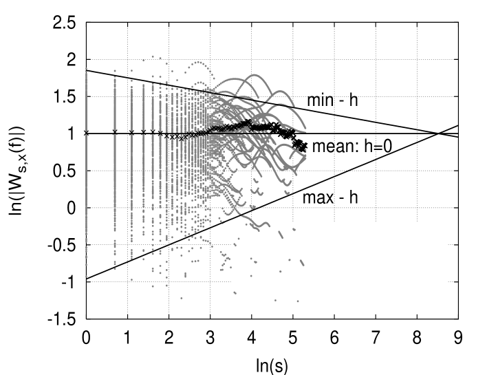
FIG. 4.: The maxima of wavelet coefficients at different scales are shown. The coefficients are bounded in the interval $-1.2<h<1.2$, [25]. The crosses indicate the mean value evaluated by using Eq. (9). The intersection point at the right is at the maximum available scale $\log(5000)=8.52$. The three straight lines indicate the slope of the mean, the maximum and minimum values of the Hölder exponents.

Figure 5

FIG. 5.: The Hölder exponents $h$ for the FGN are plotted against the position of the time series. The straight line correspond to the center of the distribution.

Figure 6

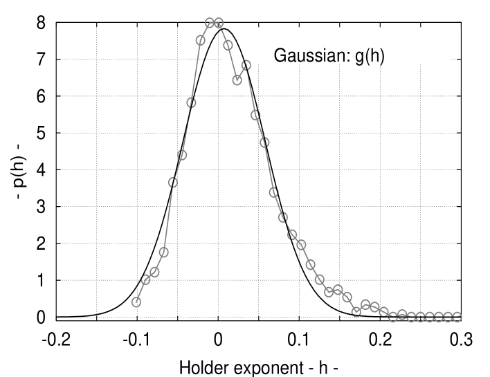
FIG. 6.: Histogram and probability density estimation of the Hölder exponents. The fitting curve is a Gaussian (15) centered in $h_{0}=0.007\pm 0.001$ and with a width $\sigma=0.051\pm 0.001$. The mean Hölder exponent given by Eq. (9) is $\overline{h}=-0.004\pm 0.008$ and correspond to the maximum of the distribution.

Figure 7

FIG. 7.: Stride interval for slow, normal and fast gait are shown. (A) The total period of time is approximately 1 hour. (B) The total period of time is 5 minutes. Note the variability of the fluctuation of the slow gait. The data is for person number 8.

Figure 8

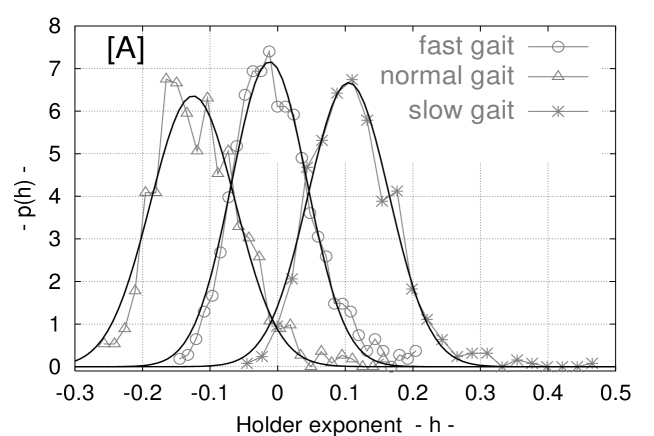
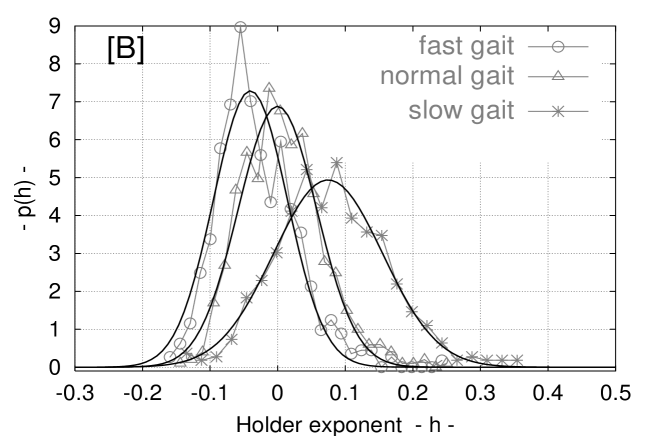
FIG. 8.: Histogram and probability density estimation of the Hölder exponents are shown for walker number 5 (A) and walker number 8 (B): slow-star, normal-triangle and fast-circle gait. By changing the gait mode from slow to normal the mean Holder exponent $\overline{h}$ decreases but from normal to fast it usually increases, but may also decrease. The fitting curves are Gaussian functions, the mean value $h_{0}$ and the standard deviation $\sigma$ are in Table 3.

Figure 9

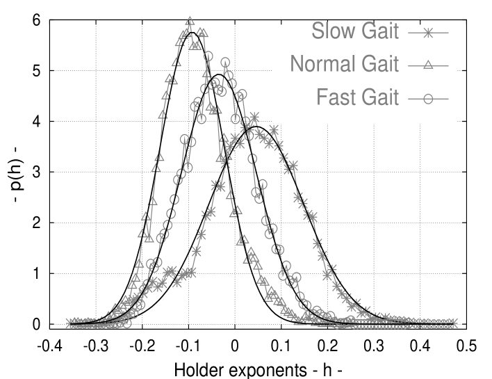
FIG. 9.: Histogram and probability density estimation of the Hölder exponents for the three walking groups are shown: slow-star, normal-triangle and fast-circle gait. By changing the gate mode from slow to normal the mean Holder exponent $h_{0}$ decreases but from normal to fast it increases. There is also an increasing of the width of the distribution $\sigma$ by moving from the normal to the slow or fast gait mode. The fitting curves are Gaussian functions, and the mean value $h_{0}$ and the standard deviation $\sigma$ are in Table 4.

Figure 10

FIG. 10.: Stride intervals for slow, normal and fast gait for metronomically triggered walking is depicted. The total period of time is approximately 30 minutes. (A) person number 3; (B) person number 5.

Figure 11

FIG. 11.: Metronomic walking. Histogram estimation of the Hölder exponents for the walker number 3 (A), and the walker number 5 (B): slow-star, normal-triangle and fast-circle gait.

Figure 12

FIG. 12.: Metronomic walking. Histogram estimation of the Hölder exponents for the three walking groups: slow-star, normal-triangle and fast-circle gait. The data shows a large range of different conditions compatible with noise from antipersistent to persistent correlations.

REFERENCES

- [1] J.B. Bassigthwaighte, L.S. Liebowitch and B.J. West, Fractal Physiology, Oxford University Press, Oxford (1994).
- [2] Z. R. Struzik, Fractals, Vol. 8, No. 2, 163-179 (2000).
- [3] http://www.physionet.org/ .
- [4] J.M. Hausdorff, P.L. Purdon, C.-K. Peng, Z. Ladin, J.Y. Wei, A.L. Goldberger, J. Appl. Physiol. 80, 1448-1457, (1996).
- [5] J.J. Collins and S.A. Richmond, Biol. Cyb. 71, 375-385 (1994).
- [6] M.D. Mann, The Nervous System and Behavior, Harper & Row, Philadelphia (1981).
- [7] A.H. Cohen, S. rossignol, and S. Grillner, Editors, Neural control of rythmic movements in vertebrates, Wiley, New York (1988).
- [8] J.J. Collins and I.N. Stewart, J. Nonlinear Sci. 3, 349-392 (1993).
- [9] Vierordt, Ueber das Gehen des Meschen in Gesunden und Kranken Zustaenden nach Selb-stregistrireden Methoden, Tuebigen, Germany (1881).
- [10] J.M. Hausdorff, C.-K.Peng, Z. Ladin, J.Y. Wei and A.L. Goldberger, J. Appl. Physiol. 78, 349-358 (1995).
- [11] B.J. West and L. Griffin, Chaos, Solitions & Fractals 10, 1519-1527 (1999).
- [12] B.J. West and L. Griffin, Fractals 6, 101-108 (1998).
- [13] L. Griffin, D.J. West and B.J. West, J. Biol. Phys. 26, 185-202 (2000).
- [14] Y. Ashkenazy, J.M. Hausdorff, P. Ivanov, A.L. Goldberger and H.E. Stanley, cond-mat/0103119 v1.
- [15] B.J. West, M. Latka and L. Griffin, submitted to PRE.
- [16] B.B. Mandelbrot, The Fractal Geometry of Nature, Freeman, New York, (1983).
- [17] I. Daubechies, Ten Lectures On Wavelets, SIAM (1992).
- [18] S. G. Mallat, A Wavelet Tour of Signal Processing (2nd edition), Academic Press, Cambridge (1999).
- [19] D. B. Percival and A. T. Walden, Wavelet Methods for Time Series Analysis, Cambridge University Press, Cambridge (2000).
- [20] S. G. Mallat, W. L. Hwang, IEEE Trans. on Information Theory 38, 617-643 (1992).
- [21] S. G. Mallat, S. Zhong, IEEE Trans. PAMI 14, 710-732 (1992).
- [22] A. Arneodo, E. Bacry, J. F. Muzy, PRE 47, No. 2, 875-884 (1993).
- [23] A. Arneodo, E. Bacry, J. F. Muzy, International Journal of Bifurcation and Chaos 4, No. 2, 245-302 (1994).
- [24] P. C. Ivanov, M. G. Rosenblum, L. A. Nunes Amaral, Z. R. Struzik, S. Havlin, A. L. Goldberger and H. E. Stanley , Nature 399, 461-465 (1999).
- [25] Z. R. Struzik, CWI Report, INS-R9803 (1998).
- [26] J. Feders, Fractals, Plenum Publishers, New York (1988).
- [27] C. Beck, F. Schlögl, Thermodynamics of chaotic systems, Cambridge university press , Cambridge, 1993.
- [28] W.H. Press, S.A. Teukolsky, W.T. Vetterling, B.P. Flannery, Numerical Recipes in C, Cambridge University Press, New York, 1997.
- [29] K. Nakamura, Quantum Chaos, Cambridge University Press, Cambridge (1993).