Exclusion particle models of limit order financial markets

Abstract

Using simple particle models of limit order markets, we argue that the mid-term over-diffusive price behaviour is inherent to the very nature of these markets. Several rules for rate changes are considered. We obtain analytical results for bid-ask spread properties, Hurst plots and price increment correlation functions.

1 Introduction

While physicists involved in academic research on financial markets have focused on the analysis and modelling of time series such as stock market prices or indices [2, 22, 11], limit order markets are addressed by economists in terms of market micro-structure [20]. In such markets, traders can publish their wish to buy/sell a given quantity of stock at a given price, that is, place a limit order. Most of the time, there is no order of the opposite type at that price, and the limit order stays in the order book until it is cancelled or matched by another order of the opposite type at the same price. An order that causes an immediate transaction, as in the last example, is called market order. One of the most interesting aspects of these markets is the interplay between price dynamics and order dynamics. Whereas economists have studied and characterised many important aspects of these markets [20], such as why traders would like to use them after all [8], and produced models with stochastic order placement (see for instance [5, 9]), physicists prefer to consider orders as particles, thinking of size as mass and price as spatial position; the price evolution merely results from stochastic dynamics: it follows a kind of random walk, hence is not assumed to be fixed or bounded in contrast with other models [25, 9, 5]. Data analysis performed in [10, 24, 6, 4, 35] shows that in the language of physics, limit order markets are out-of-equilibrium, that is, there are similar to a bucket of water heated by a campfire and filled by an irregular shower. There are two families of nonequilibrium particle models of such markets, one that assumes that orders diffuse on the price axis [1, 14, 33] and another one where orders can be placed, executed [5, 23] and cancelled [6, 12, 4]. There is evidence from market data that orders do not diffuse on the price axis, but are placed, and then executed or cancelled with time dependent rates [6]. This begs for a non-equilibrium model made up of these three processes [6, 12, 4]. So far, all models have assumed constant rates. Here we show that this assumption is responsible for very unrealistic price behaviour, and that lifting this assumption leads to the correct behaviour.

It is well documented that stock and foreign exchange prices are over-diffusive over several months [26, 11]: if the (log)-price $p_{t}$ followed a standard random walk, its increments (or returns) would be such that $p_{\tau}-p_{0}\sim\tau^{H}$ with $H=1/2$; $H$ is called the Hurst exponent. Generally speaking, $H$ depends on $\tau$. For instance, real prices are reportedly over-diffusive ($H>1/2$) for several months, and then tend to be diffusive ($H=1/2$) for larger time lags [26, 11]. Over-diffusion implies some sort of long-term memory. This behaviour is not captured in the current particle models. On the contrary, $H=1/4$ for all times in models where no cancellation of orders is allowed [1, 14, 23]. It has been realised that order cancellation is needed in order to obtain a crossover to diffusive price for large time lags [6]. On the other hand, over-diffusive behaviour is obtained when price trends are introduced, that is, when the price has a temporary tendency to rise or decrease, as in the model of Ref. [33], which has $H=2/3$ for all times, when no order cancellation is allowed, and a crossover to $H=1/2$ when it is. Here we generalise the notion of trends introduced in [33], and study their influence on the Hurst exponent and the return correlation function.

Nonequilibrium particle models are notoriously hard to tackle analytically, and limit order market models are no exception. Therefore one ought to study first the simplest models of this kind, namely exclusion models [33], where at most one order is present at each tick. Recent work in nonequilibrium statistical mechanics shows that some of these particle models can be exactly solved [13] (see [31] for a review). Exclusion is naturally found when there are so few orders that it is unlikely to find two orders at the same tick, which is also the limiting case where Ref [30] obtained analytical results concerning order densities in a class of models introduced in [6, 12]. Beyond this seductive mathematical aspect, exclusion models are arguably relevant for the modelling of limit order market. Indeed, priority of execution is given to orders first by price and then by chronological order of their deposition. This is particularly important near the best prices, when impatient traders are likely to be willing to take precedence over their colleagues. Therefore exclusion models of limit order markets capture at least some part of the dynamics near the bid-ask spread, which plays a major role in these markets, particularly when there is no market maker. Another interpretation of the exclusion condition is that it encodes the presence or absence of quotes at a given tick and neglects the actual number of shares.

In short, the exclusion hypothesis is a way to reduce the dimensionality, hence the complexity, of limit order market models, while keeping their collective character. Here we transform the particle model found in Ref. [6] by identifying processes in real markets into an exclusion model.

2 Definition of the model

Two types of orders, ask ($A$) and bid ($B$), also denoted by $-$ and $+$ and corresponding respectively to sell and buy orders, live on a semi-infinite line — the price whose unit is the tick. As limit orders are a way of storing demand and offer, it is clear that all bid orders are found on the left of the ask orders. At time $t$, there are $n_{i}(t)\in\{-1,0,1\}$ orders on site $i$, where $-1$ denotes the presence of an ask order and $1$ the presence of a bid order. We denote by $b(t)$ the position of best bid price and $a(t)$ the position of the best ask price. The last paid price $p(t)$ is the position where a transaction last took place. All quantities of interest depend on these last three quantities. For instance, the bid-ask spread is the gap that separates the best bid from the best ask; here we denote it by $s(t)=a(t)-b(t)-1$. We do not consider any mechanism which would ensure the positivity of the price, since we aim to study normal price dynamics; we argue that special mechanisms arise in real markets when the price reaches very low prices. We assume that all processes occur relative to the current best prices, that is, relative to $a(t)$ for asks and $b(t)$ for bids. At each time step $t$, three different events can happen: a new order of each type (bid+ask) is placed, a market order of each type is placed, and some orders are cancelled. Mathematically,

1. with probability $\delta_{a}$, a new ask order is placed into the bid-ask spread. Its price $a(t)-\Delta$ ($\Delta>0$) is randomly drawn according to some distribution probability $P_{a}(\Delta)$. With probability $\delta_{a}^{\prime}$, another ask order is deposited on the right of the current best price at $a(t)+\Delta^{\prime}$, where $\Delta^{\prime}>0$ is randomly drawn from $P_{a}^{\prime}(\Delta^{\prime})$. Idem for bids: an new order is placed in the spread with probability $\delta_{b}$ at $b(t)+\Delta$, where $\Delta$ is taken from $P_{b}(\Delta)$. With probability $\delta_{b}^{\prime}$, a new order is placed at a lower price that $b(t)$, that is, at $b(t)-\Delta^{\prime}$ where $\Delta^{\prime}$ is drawn from the probability distribution function (pdf) $P_{b}^{\prime}(\Delta^{\prime})$. There can be at most one order per site, hence, if there is already a particle at $b(t)-\Delta^{\prime}$, or at $a(t)+\Delta^{\prime}$, nothing happens.

2. Each particle has the same fixed probability $\eta$ to be cancelled.

3. With probability $\alpha_{a}(t)$ a market order eats the best ask order located at $a(t)$ and with probability $\alpha_{b}(t)$ the bid order at $b(t)$ is executed.

4. Rates change according to predefined rules (see below).

Deposition and market orders in particle limit order market models can be found in Ref. [23], cancellation was introduced in Ref. [6] and in Ref. [9] in a different context; its main role is to ensure that the total number of orders does not diverge with time. Note that $P(\Delta)$ has a major influence on the bid-ask spread dynamics; the average typical deposition position conditional to the bid-ask spread depends linearly on the spread in real markets [6], which we denote by $\langle{\Delta^{2}|s(t)}\rangle^{1/2}=c_{0}+c_{1}s(t)$, where $\langle{.}\rangle$ denote a temporal average. This can be explained for instance by buy orders that are placed at $b(t)+s(t)/2$, or very close to the best ask order, e.g. at $a(t)-1$. Playing with $c_{0}$ and $c_{1}$ modifies the spread dynamics. For instance, if $c_{0}>0$, $c_{1}=0$, there is no feed-back of the spread on the width of deposition; if $c_{1}>1$, the contribution of cross-deposition to market orders cannot be neglected. Finally, if $c_{0}=0$ and $c_{1}>0$, the cross-deposition rate is constant.

Several simplifying hypotheses will be made here: we will assume that all deposition pdfs are equal, that is, $P_{a}=P_{b}=P_{a}^{\prime}=P_{b}^{\prime}$, and Gaussian. This contrasts with empirical facts that $P^{\prime}(\Delta)$ is a power-law over two decades of ticks in the Paris Bourse [4] in the London Stock  [35], and in the NASDAQ [27], which implies that the probability of far deposition is non-negligible. In addition, the cancellation rate of a given order has a power-law dependence on its position relative to the best order, $\eta(\Delta)\sim\Delta^{-\nu}$ with $\nu\simeq 2$ [27], which is consistent with the functional form of the lifetime distribution previously reported [19, 6]: here, this dependence is neglected.

In real markets, rates are not fixed, but vary wildly during any trading day. Moreover, we see no practical reasons why the rates should obey a balance equation such that the expected price drift is zero at all times, as it is assumed in all current models, except that of Ref. [33]. On the contrary, heterogeneity of market participants is probably enough to argue that rates should be balanced only on average. As a first approximation, we assume here that they are independent from each other. As we shall see, this provides a universal mechanism for mid-term over-diffusive prices. We study several alternative simple rules that stipulate how to change the rates, depending on the quantity to be computed:

1. At each time step, with probability $p$, all rates are redrawn independently at random. The Hurst exponent is then very easy to compute.

2. At each time step, each rate is redrawn with probability $p$. This is also appropriate for the computation of the Hurst exponent.

3. Rates are linearly cross-correlated, that is,

   $$\alpha_{a}(t)=\alpha_{0}+\alpha_{1}\sigma(t) \alpha_{b}(t)=\alpha_{0}-\alpha_{1}\sigma(t)$$ (1)

   $$\delta_{a}(t)=\delta_{0}-\delta_{1}\sigma(t) \delta_{b}(t)=\delta_{0}+\delta_{1}\sigma(t),$$ (2)

   where $\sigma(t)=\pm 1$ is the only quantity that is changed with probability $p$ at each time step. It defines the direction of trend. This setup makes it easy to compute the autocorrelation function and the properties of the bid-ask spread.

4. Same as rule (iii), with the additional constraint that $\alpha_{0}=\alpha_{1}$ and $\delta_{0}=\delta_{1}$. In this case, market orders occur at one side, and order deposition at the other.

5. Same as rule (iv), but the direction of the trend $\sigma(t)$ is allowed to change only when the bid-ask spread is zero [33].

In rules (i-iv) the probability of rate change at each time step is constant. This sets the typical lifetime of a set of rates to $1/p$, and that rates are exponentially cross- and auto-correlated, whereas this dependence should be algebraical [6, 16]. Rule (v) relates trend changing to the actual properties of the bid and ask distribution. Other similar rules could also be studied, for instance by relating probabilistically the trend to volume imbalance between the two distributions. However, rule (v) is most appropriate for mathematical analysis.

3 Bid-ask spread properties

Here we derive basic results about the bid-ask spread. We assume that the width of order deposition does not depend on the bid-ask spread ($c_{1}=0$), and that the price of new orders new prices $a(t)-1$ and $b(t)+1$, that is, $P(\Delta)=\delta_{\Delta,1}$ where $\delta$ is the Kronecker index. Finally, we neglect cancellation, whose role is less crucial in exclusion models, as the exclusion condition itself limits the total number of orders. The last two assumptions imply that after a transient [36], the order density is uniform and equal to $1$ for $p<b(t)$ and $p>a(t)$.

As long as the rates are fixed, the best ask evolution is the following: $P[a(t+1)=a(t)+1]=\alpha_{a}$, and $P[a(t+1)=a(t)-1]=\delta_{a}$, hence $a(t)$ follows a biased random walk (RW) with drift $\alpha_{a}-\delta_{a}$. The same applies to $b(t)$, with a drift of $\delta_{b}-\alpha_{b}$, hence the mid-price, defined as $m(t)=(a(t)+b(t))/2$, diffuses with an average drift $(\alpha_{a}+\delta_{b}-\alpha_{b}-\delta_{a})/2$. The evolution of the spread $s(t)$ is also a biased RW, with drift $v=\alpha_{a}+\alpha_{b}-\delta_{a}-\delta_{b}<0$. Since $s(t)\geq 0$, the spread undergo a biased RW with reflective boundary at $s=0$. Several properties of $s$ can then be easily computed. For instance the pdf of the time during which $s>0$ is given by the first passage at $s=0$ of a particle starting at $s_{0}$ [28]

$$F(t)=\frac{s_{0}}{\sqrt{4\pi Dt^{3}}}\exp\left[-\frac{(s_{0}+vt)^{2}}{4Dt}\right].$$ (3)

where $D$ is the diffusion constant. In particular, when $v\to 0_{-}$, $F(0,t)\simeq t^{-3/2}$. For any $v<0$, it is well known that the pdf $P(s,t)$ of random walks with reflective boundary tends to a stationary state that is exponentially decreasing

$$P(s)=\frac{|v|}{D}\,\exp(-|v|s/D)$$ (4)

and $\overline{s}=D/|v|$, where $\overline{.}$ denotes an average over $P(s)$. As shown by these equations, the spread properties only depend on $v$ and $D$, provided that $v$ and $D$ remain constant long enough.

Rules (iii), (iv) and (v) for rate change are such that the change of trend $\sigma(t)$ has no influence on the dynamics of $s(t)$, as $v$ and $D$ are independent of $\sigma(t)$, therefore the above equations are always valid in this case. In particular, rule (iv) makes the spread dynamics a one-step process for $s>0$:

$$\frac{dP(s)}{dt} = [(1-\delta)(1-\alpha)+\alpha\delta]P(s)$$ (5)

$$+\delta(1-\alpha)P(s+1)+(1-\delta)\alpha P(s-1)$$

Note that for $s=0$, any deposition is in fact a cross-deposition, hence the effective annihilation rate $\alpha_{\rm eff}$ equals $\alpha+\delta$. Eq. (5) shows again that the spread process is equivalent to a biased RW with reflective boundary at $s=0$; its drift is $v=\alpha-\delta<0$, and its diffusion constant $D=[\alpha(1-\alpha)+\delta(1-\delta)]/2$. If order cancellation is allowed, the 0-th order correction to the above picture is $\delta\to\delta-\eta$ and $\alpha\to\alpha+\eta$, hence $v\to v-2\eta$.

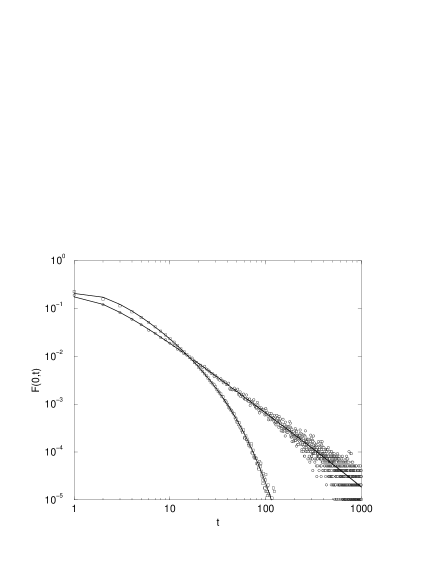
Figure 1: Trend duration pdf $F(0,t)$, for rule (iv) ($s_{0}=1$, $\delta=0.5$, $\alpha=0.20$ (squares) and $\alpha=0.48$ (circles)). $10^{7}$ iterations. Continuous lines are theoretical predictions from Eq (3).

4 Hurst exponent

The Hurst exponent $H$ depends in general of $\tau$ in our model. Irrespective of the considered rule for the update of the rates, the price is over-diffusive ($H>1/2$) for intermediate $\tau$ and diffusive ($H=1/2$) for large $\tau$. For rules (i)-(iv), the crossover between $H>1/2$ and $H=1/2$ occurs for $\tau\sim 1/p$. When rule (v) is applied, it occurs for $\tau$ of the order $\int dtF(0,t)t$. The small $\tau$ behaviour depends on the rule and on the parameters, as discussed below.

4.1 Rule (i)

The simplest setup for computing the Hurst exponent $H(\tau)$, is to change the rates according to rule (i). For a given set of rates $\alpha_{a}$, $\alpha_{b}$, $\delta_{a}$, $\delta_{b}$, the average speed of the mid-price $m(t)$ is $v=\alpha_{a}+\delta_{b}-\alpha_{b}-\delta_{a}$. Neglecting the diffusion of the mid-price, and retaining only its ballistic motion, one readily computes $\langle{r(t+\tau)r(t)}\rangle\sim(1-p)^{\tau}$. Therefore, after a summation,

$$\langle{(p_{t+\tau}-p_{t})^{2}}\rangle=\langle{(\sum_{t^{\prime}=1}^{\tau}r_{t+t^{\prime}})^{2}}\rangle\sim\tau+\frac{2(1-p)}{p^{2}}\,\left[p\tau-1+(1-p)^{\tau}\right],$$ (6)

Figure 2 shows that Eq (6) describes adequately the price behaviour for large $\tau$. The discrepancy observed for small $\tau$ is probably due to bid-ask spread bouncing and other diffusive behaviours that we neglected. Note that when the deposition rates are close on average to the market order rates, a sub-diffusive behaviour appears for small times. This general behaviour is due to spread bouncing, as in this case, the spread is typically large. It appears for all rules where frequent spread bouncing is allowed, owing to the possibility of having simultaneous market orders at both sides, that is, rules (i), (ii) and (iii).

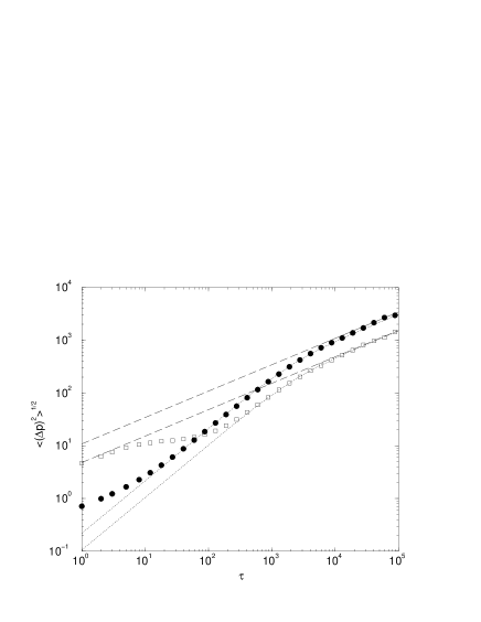
Figure 2: Hurst plot of the price increments for rule (i). . Market order rates drawn uniformly between 0 and 0.1, deposition rate between 0 and 1 (circles), 0 and 0.5 (squares). $p=0.001$, $10^{6}$ iterations, no order cancellation. The dashed line represents normal random walk ($H=1/2$) and dotted lines are obtained from Eq. (6).

Figure 3: Hurst plot for rule (iii), showing characteristic under-diffusive prices at short times. ($\delta=0.5$, $\alpha_{0}=0.22$, $\alpha_{1}=0.02$, $\eta=0$, $p=0.001$, $0.01$ and $0.1$, $10^{6}$ iterations)

4.2 Rule (ii)

Rule (ii) is arguably more realistic than rule (i). While it leads to essentially the same behaviour, the calculus is more complicated and of no special interest for our purpose.

4.3 Rule (iii)

Fig. 3 shows that, similarly to rule (i) and (ii), if $p$ is small enough, the price is under-diffusive, then over-diffusive, and tends to be diffusive at large times. Since the duration of the over-diffusive part is related to $1/p$, when $p$ is too large, the price cannot develop its over-diffusive behaviour. Note that the crossover from $H>1/2$ to $H=1/2$ has the same characteristic form as in Figs 2 and 4.

4.4 Rule (iv)

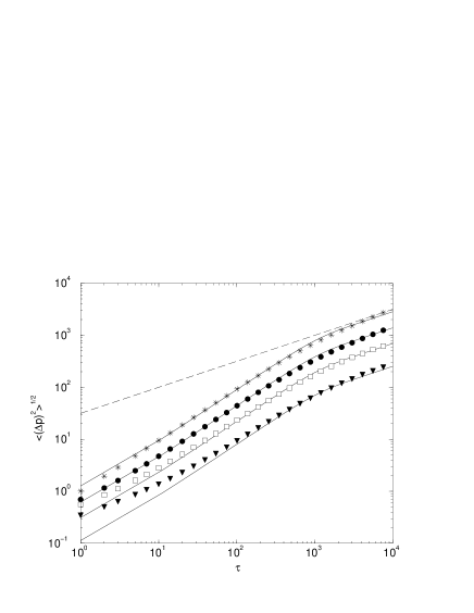
Figure 4: Hurst plot for rule (iv) for $\alpha=0.9$, $\delta=1$ (stars), $\alpha=0.44$, $\delta=0.5$ (circles), $\alpha=0.22$, $\delta=0.25$ (squares), and $\alpha=0.08$, $\delta=0.1$ (triangles) ($p=0.001$, $\eta=0$ and $10^{6}$ iterations in all datasets).

In the case of Rule (iv), the price follows a persistent RW [32], that is, the probability that $r(t+1)=r(t)$ is equal to $1-p$, where $p$ is the probability of trend reversal. Therefore, the over-diffusive behaviour of our model can be qualitatively explained by mapping the price increments ($\pm 1$) to an unidimensional (nearest neighbour) Ising spin model where the space plays the role of the time. A spin is a variable that can take two values $-1$ and $+1$ (think of a price increment). The unidimensional Ising model consists in placing a given number of these on a line, and to assuming that spin at site $i$ is only influenced by its neighbours, that is, the spins at sites $i+1$ and $i-1$ (see [34] for more information). The mapping is possible, because the market model we consider is Markovian. Generalising known results for such models to our case where the price jumps over the spread when the trend reverses, whose effect turns out to be negligible for large $\tau$, we find when $p$ is small and $\langle{s}\rangle\ll 1/p$ that for large $\tau$,

$$\langle{[p(t+\tau)-p(t)]^{2}}\rangle\simeq\alpha^{2}\left[\tau+\frac{\tau(1-p)}{p}\tanh[\tau p/(1-p)]\right]~{}~{}~{}\tau\gg 1$$ (7)

which indicates a continuous crossover between $H(\tau)=1$ for small $\tau$ and $H=1/2$ for large $\tau$. However, the crossover appears visually to occur in a small time window. The mapping between the market and Ising models gives good results, even for small $\tau$.

4.5 Rule (v)

This rule also gives rise to a persistent RW, hence to the same results as those of rule (iv).

5 Price autocorrelation

In this section, we study how the price increments autocorrelation function $C(\tau)=\langle{r(t+\tau)r(t)}\rangle$ depends on the rule of rate changes and on the chosen parameters.

5.1 Rule (iv)

Suppose that the probability of trend reversal is equal to $p$ at each time step. Neglecting the effect of cross-deposition when $s=0$, we find

$$C(1)\simeq C_{0}(1) = \alpha^{2}[(1-p)^{2}-p(1-p)(1-\delta)$$ (8)

$$-p^{2}(\langle{s^{2}}\rangle+\langle{s}\rangle(1-\delta))].$$

As soon as the influence of spread bouncing is greater than that of annihilation, $C(1)<0$. This is to be related to one known possible cause for negative $C(1)$, spread bouncing [29, 11], although here it only happens whenever the trend $\sigma(t)$ changes. When $P_{s}(0)$ is not negligible, Eq (8) must be corrected: a transaction takes place if a market order is placed ($\alpha$), or a market order is deposited onto the best opposite order ($\delta$) (cross-deposition). If both happen during a time-step, we assume that annihilation occurring before and after deposition are equally likely. We finally find

$$C(1) \simeq (1-P_{s}(0))C_{0}(1)$$ (9)

$$+P_{s}(0)\{(1-p)^{2}\alpha[\alpha+\delta(1-\alpha/2)(1+\delta/2)]$$

$$+p(1-p)[\alpha^{2}\delta/2-\alpha(\alpha+\delta+\alpha\delta^{2}/4)]-p^{2}\alpha\delta^{2}\}$$

Figure 5 shows that numerical simulations are in good agreement with Eq (9). Note that for this figure we used values of $P_{s}(0)$, $\langle{s}\rangle$ and $\langle{s^{2}}\rangle$ directly taken from the simulations, as the continuous approximation for $P_{s}$ breaks down for typically small spreads. In the right panel, the typical spreads is very small and $C_{0}(1)$ is not a good approximation to $C(1)$. Eq (9) relates the price increments autocorrelation function to the average spread and the second moment of the spread, hence, can be seen as a generalisation of the seminal result of Ref [29], and is related other works [21, 17].

Figure 5: Price increment autocorrelation function $C(1)$ of the model of subsection 5.1 (left panel: $\delta=0.5$, $\alpha=0.4$; right panel: $\delta=0.8$, $\delta=0.4$. $\eta=0$, average over $50$ runs, 10⁵ iterations; continuous lines are theoretical predictions of Eq (9), and dashed lines are those of Eq. (8)).

5.2 Rule (iii)

Simultaneous transactions on both sides of the market are an additional source for short term negative return autocorrelation. Results of the previous subsection can be generalised to this case: the spread dynamics is described by a two-step process, which is again equivalent to a biased random walk with reflective boundary at $s=0$, and $C(1)$ can be calculated, but leads to expressions too long to be reported here.

5.3 Rule (v)

Ref. [33] studies a particle exclusion market model where the order diffuse toward best prices and the rates are changed according to rule (v). According to the previous section, the trend duration pdf in this model is given by Eq (3) (see also Fig. 1); in addition, the rates are tuned so as to ensure that $v=0$. Therefore the trend duration has no definite average, which explains intuitively why without order cancellation the price is always over-diffusive in this model; on the other hand, when order cancellation is allowed, the effective rates have to be corrected; this yields an effective $|v|=2\eta>0$, which is the origin of the crossover to diffusive prices observed in this case. Because this rule does not allow spread bouncing, the absolute value of price increments is 0 or 1, and the sign of the increment stays constant for a duration $F(l)$ that is given by Eq (3). According to Ref. [15], the increment autocorrelation $C(\tau)$ of such processes is the inverse Laplace transform of

$$\hat{C}(s)=\frac{1}{s}\left[1-2\frac{1-\hat{F}(s)}{s\langle{l}\rangle(1+\hat{F}(s))}\right]$$ (10)

where $F(l)$ is the pdf of trend duration $l$. Unfortunately, $\hat{C}(s)$ cannot be inverted for $F$ given by Eq (3). However, one can argue from this equation that for $\tau$ small enough, $C(\tau)\sim\tau^{-1/2}$, following Ref. [3]. Another possibility is to consider a standard biased RW starting from $s_{0}$ and compute the probability that $s(t)<0$, neglecting the effects of the reflective boundary, which leads to

$$\langle{r(t)r(t+\tau)}\rangle=1-2P[r(t)=-r(t+\tau)]\simeq{\rm erf}\,\left[\frac{v\tau+s_{0}}{\sqrt{2D\tau}}\right]$$ (11)

where the last approximation is valid as long as $v\tau+s_{0}\gg 0$, that is, as long as the spread is not likely to have reached the reflective boundary. When $\tau$ is such that $\frac{v\tau+s_{0}}{\sqrt{2Dt}}\ll 1$, that is $\tau\ll 2D/|v|$, $\langle{r(t)r(t+\tau)}\rangle\propto\tau^{-1/2}$, with a cutoff at $t\sim 2D/|v|$. Note that this result is exact if $v=0$, and gives $\langle{r(t)r(t+\tau)}\rangle\sim\tau^{-1/2}$ for $\tau\gg s_{0}^{2}/2D$, in agreement with Ref [33]. The problem of this approach is that it gives positive autocorrelation for all times, whereas it is negative at short times in real markets [11].

6 Price increment distribution

All rules, except rule (v), lead to the same kind of price increment pdf, which is made up of one part that is due to consecutive market orders on the same side, and another that is due to spread bouncing (the price pdf produced by rule (v) lacks the spread bouncing part). This implies that when the rates are constant, the tails of $P(r)$ are given by that of the spread pdf, which decreases exponentially in that case. In other models, found e.g. in Refs [23, 6], the pdf of the spread is fat-tailed, hence that of the prices as well, which is arguably artificial, since the mid-price increments $m(t)$ are also fat tailed in real markets [11].

It is possible to obtain a more refined pdf of the trends. Up to here we essentially considered constant rates, which lead to exponential tails. Time varying rates is the key to obtain fat tailed return pdf in these models: the mid-spread point $m$ moves indeed at average speed $\frac{(\delta_{B}-\alpha_{B})+(\alpha_{A}-\delta_{A})}{2}=(\alpha_{0}+\alpha_{1}+\delta_{0}+\delta_{1})\sigma$. The rates are in principle not bounded, as it is easy to generalise our model to include multiple order depositions/annihilations during a time step. In this case, they indicate the average number of events during $\Delta t=1$ of a Poisson process. Their distribution is related: about 10% of deposited orders are matched in the London Stock Exchange [10] as well as in the ISLAND ECN (www.island.com), a subpart of the NASDAQ [6], hence one can consider the deposition rate as proportional to the annihilation rate in a first approximation. $P(r)$ has fat tails as soon as $P(\alpha)\sim\alpha^{-\gamma}$. According to Ref. [16], this is the case, with an exponent of about $3.5$. In addition, the autocorrelation of all the rates was found to be algebraically decaying [6], which also shows up in that of the number of transaction in a given time interval [16]. We shall explore further this generalisation in a forthcoming publication.

7 Average densities

Two recent papers [12, 4] have focused on the average densities of orders relative to the best prices. In both cases, these were found to have power law tails. The model of Ref. [6] and its exclusion version, i.e. the model proposed here with spread-feedback, are able to reproduce this behaviour (see fig 6); $\langle{B(\Delta)}\rangle$ is very well fitted with the functional shape $(1+ax)^{b}$ with $b\simeq-2.03$, very close to $-2$. This gives a market impact exponent of $1/2$, which was measured in real markets, as reported Ref [18]. Note that the model of Ref. [12] also gives the same exponent: this model can be seen as a special case $c_{1}=1/\sqrt{2}$, $c_{0}=0$ of Ref. [6], with a flat spatial probability distribution of deposition; in particular, spread-feedback is present ($c_{1}>0$), which seems to be necessary for obtaining densities with power-law tails.

Interestingly, the functional shape of the average densities is the same as that of the price in these models. In fact, it is also the same as that of the spread, a general feature of market models with constant rates, as explained above. This last feature is probably very unrealistic, as the pdf of the spread is most likely exponential in real markets. Nevertheless, this can be easily explained. Suppose that the spread pdf has power tails, then order deposition pdf has fat tails, hence, according to the argument developed in ref [4], the average densities have power-law tails. In addition, as before, when the rates are constant, the tails of the price pdf are due to spread bouncing, hence are also fat. In conclusion, in this type of models, the spread, the price and the densities have all the same type of pdf. But as argued above, fat tailed return should be obtained by modulating the rates. Note that the model of Ref. [4] produces power-law tails for the densities by considering power-law distributed relative positions for bulk deposition, which is consistent with empirical findings.

Figure 6: Integrated average bid density $\langle{B}\rangle(\Delta)$ versus $\Delta$, the position relative to the best bid for $\eta=0.01$ and spread feed-back ($\delta=0.5$ $\alpha=0$, $c_{0}=2$, $c_{1}=3$). The dashed line has an exponent of -1.

8 Conclusions

The simplest particles models of limit order markets are exclusion models and provide an ideal framework for mathematical analysis. We argued that particle models of limit order market should include time-varying rates, and that the balance of rate only holds on average, and is a crucial feature of these markets, explaining mid-term over-diffusive price behaviour. We introduced several rules for time varying order deposition and market order rates and characterised the bid-ask spread properties, computed Hurst plots and correlation functions. The effects of order cancellation and more general probability distributions of rates will be addressed in the future.

This work was supported by EPSRC under Oxford Condensed Matter Theory grant GR/M04426. We thank G. M. Schütz for seminal discussions.

References

- [1] Bak. P., Shubik M., Pakzuski M., Price Variations in a Stock Market With Many Agents, Physica A 246, 430 (1997), e-print cond-mat/9609144
- [2] Bouchaud J.-Ph. and Potters M., Theory of Financial Risks, Cambridge University Press, Cambridge (2000)
- [3] Bouchaud J.-Ph. , Giardina I., Mezard M., On a universal mechanism for long ranged volatility correlations Quantitative Finance 1, 212-216 (2001), e-print cond-mat/0012156
- [4] Bouchaud J.-Ph., Mézard M., Potters M., Statistical properties of stock order books: empirical results and models, Quantitative Finance 2, 251 (2002), e-print cond-mat/0203511
- [5] Bollerslev T., Domowitz I., Order Flow and the Bid-Ask Spread: An Empirical Probability Model of Screen-Based Trading, Journal of Econ. Dynamics and Control 21, 1471 (1994)
- [6] Challet D., Stinchcombe R., Analyzing and modelling 1+1d markets, Physica A 300, 285, (2001), e-print cond-mat/0106114
- [7] Chan D. L.C., Eliezer D., Kogan I. I., Numerical analysis of the Minimal and Two-Liquid models of the Market Microstructure, e-print cond-mat/0101474 (2001)
- [8] Cohen K. et al, Transactions Costs, Order Placement Strategy and Existence of the Bid-Ask Spread, Journal of Political Economy 89, 287 (1981)
- [9] Cohen K. J, Conroy R. M., Maier S. F:, Order flow and the quality of the market, in: Y. Amihud, T. Ho and R. Schwartz, eds., Market Making and the Changing Structure of the Securities Industry, 1985, Lexington Books, Lexington MA
- [10] Coppejans M., Domowitz I., Screen Information, Trader Activity and Bid-Ask Activity in a Limit Order Market, preprint (1999), available at http://www.smeal.psu.edu/faculty/ihd1/Domowitz.html
- [11] Dacorogna M. M. et al. An Introduction to High-Frequency Finance, Academic Press, London (2001)
- [12] Daniel M. G. et al. How storing supply and demand affects price diffusion, e-print cond-mat/0112422
- [13] Derrida B. et al., Exact solution of a 1D asymmetric exclusion model using a matrix formulation, Journal of Physics A 26, 1493 (1993)
- [14] Eliezer D., Kogan I. I. , Scaling Laws for the Market Microstructure of the Interdealer Broker Markets, Capital Markets Abstracts, Market Microstructure 2, 3 (1999), preprint cond-mat/9808240
- [15] Godrèche C., Luck J. M., Statistics of the occupation time of renewal processes, e-print cond-mat/0010428
- [16] Gopikrisnan P. et al., Statistical Properties of Share Volume Traded in Financial Markets, Physical Review E 62, R4493 (2000), e-print cond-mat/0008113
- [17] Huang, R., Stoll, H., The components of the bid-ask spread: a general approach. Review of Financial Studies 10, (1997)
- [18] Lillo F., Farmer J. D., Mantegna R., Single Curve Collapse of the Price Impact Function for the New York Stock Exchange, e-print cond-mat/0207428
- [19] Lo A., MacKinlay C, Zhang J., Econometric Models of Limit-Order Executions, Journal of Financial Economics 65, 31-71 (2002)
- [20] Madhavan A., Market microstructure: A survey, Journal of Financial Markets 3, 205 (2000)
- [21] Madhavan A., Richardson M., Roomans M.. Why do security prices fluctuate? a transaction- level analysis of NYSE stocks. Review of Financial Studies 10, 1035 (1997) %bibitemSupriya Majumdar S. N., Krishanmurthy S., Barma
- [22] Mantegna R. and Stanley H. G., Introduction ot Econophysics, Cambridge University Press, Cambridge, 2000.
- [23] Maslov S., Simple model of a limit order-driven market, Physica A 278, 571 (2000), e-print cond-mat/9910502
- [24] Maslov S., Mills M., Price fluctuations from the order book perspective - empirical facts and a simple model, Physica A 299, 234 (2001), e-print cond-mat/0102518
- [25] Mendelson H., Market behavior in a clearing house, Econometrica 50, 1505 (1982).
- [26] Plerou V. et al., Economic Fluctuations and Diffusion, Physical Review E 62, R3023 (2000) e-print cond-mat/9912051
- [27] Potters M., J.-Ph. Bouchaud, More statistical properties of order books and price impact, e-print cond-mat/0210710
- [28] Redner S., A guide to first-passage processes, Cambridge University Press, Cambridge MA (2001)
- [29] Roll R., A simple implicit measure of the effective bid-ask spread in an efficient market, Journal of Finance 39, 1127 (1984)
- [30] Smith E. et al., Theory of continuous double auction, e-print cond-mat/0210475 (2002)
- [31] Stinchcombe R., Stochastic non-equilibrium systems, Advances in Physics 50, 431 (2001)
- [32] Weiss G. H. , Aspects and Applications of the Random Walk, North-Holland, Amsterdam, (1994)
- [33] R.D. Willmann, G.M. Schütz, D. Challet, Exact Hurst Exponent and Crossover Behavior in a Limit Order Market Model, Physica A 316, 526 (2002), e-print cond-mat/0206446
- [34] Yeomans J. M., Statistical Mechanics of Phase Transitions, Oxford University Press, Oxford (1992)
- [35] Zovko I., Farmer J. D., The power of patience: A behavioral regularity in limit order placement, Quantitative Finance 2, 387 (2002), e-print cond-mat/0206280
- [36] More precisely, if or .