Potential of Mean Force between a Spherical Particle Suspended in a Nematic Liquid Crystal and a Substrate

Abstract

We consider a system where a spherical particle is suspended in a nematic liquid crystal confined between two walls. We calculate the liquid-crystal mediated potential of mean force between the sphere and a substrate by means of Monte Carlo simulations. Three methods are used: a traditional Monte Carlo approach, umbrella sampling, and a novel technique that combines canonical expanded ensemble simulations with a recently proposed density of states formalism. The latter method offers clear advantages in that it ensures good sampling of phase space without prior knowledge of the energy landscape of the system. The resulting potential of mean force, computed as a function of the normal distance between the sphere and a surface, suggests that the sphere is attracted to the surface, even in the absence of attractive molecular interactions.

I Introduction

The alignment of nematic liquid crystals can be controlled by surface chemistry or topography on the scale of a few nanometers. When the uniform alignment is disturbed, this event can be detected through the appearance of multidomains in an optical microscope between cross-polarizers. One possible event that can trigger this transition is the binding of a protein or a virus to the surface, thereby providing the basis for development of sensors gupta98 ; vannelson02 . Recent experiments have in fact shown that such liquid crystal sensors are remarkably sensitive to the presence of minute amounts of protein on a substrate gupta98 ; vannelson02 .

Several experiments using colloids in bulk or confined liquid crystals have studied the influence of local disturbances in a nematic host poulin97 ; poulin98 ; gu00 . Colloidal particles in liquid crystals have also been studied by computer simulations billeter00 ; andrienko01 . One of the questions that arises from these experiments pertains to the nature of the liquid crystal mediated interaction between the colloids, or a colloidal particle and a surface.

This interaction can be quantified through a potential of mean force; molecular simulations provide a means to calculate it directly by fixing or constraining a reaction coordinate of interest. In the particular case of liquid crystals, however, conventional simulation techniques such as Monte Carlo (MC) or molecular dynamics (MD) in regular ensembles are limited in their ability to sample phase space. The system can be trapped in local energy minima and, for MD simulations, the time scales associated with the motion of the colloid can be prohibitively long.

The majority of available methods for measuring the potential of mean force either require prior knowledge of the free energy of a system roux94 ; engkvist96 ; vondele00 , or constrain the system to a limited range of the reaction coordinate straatsma92 ; sprik98 . A novel method is proposed in this work to calculate the potential of mean force which does not require prior knowledge of the free energy and permits efficient sampling. The proposed technique consists of an expanded ensemble in the reaction coordinate, implemented within the formalism of a recently proposed density-of-states sampling technique wang01a . Related methods have been proposed by de Oliveira et al. deoliveira96 and by Engkvist et al. engkvist96 . This method is applied here to determine the potential of mean force between a spherical colloidal particle suspended in a confined nematic liquid crystal and a wall.

II Simulation Methods

II.1 Potential of Mean Force

The potential of mean force (PMF) provides a measure of the effective difference in free energy between two states as a function of one or several “interesting” degrees of freedom. These degrees of freedom can be real coordinates of the system or a combination of them. They are often called reaction coordinate(s) $\xi$. An integration of the derivative of the Hamiltonian with respect to the coordinate of interest is performed along the reaction coordinate to provide a local estimate of the PMF, $w$, between two points $\xi_{1}$ and $\xi_{2}$:

$$w(\xi_{2})-w(\xi_{1})=\int_{\xi_{1}}^{\xi_{2}}d\xi^{\prime}\biggl{\langle}\frac{\partial H}{\partial\xi}\biggr{\rangle}$$ (1)

The reaction coordinate $\xi$ need not be directly observable, in the case of chemical reactions, for example, it can be the extent of reaction, and the potential of mean force provides a measure of the activation energy. It can also be a physical coordinate, such as the distance between two solute molecules in a solvent—the PMF then reflects the work required to bring two solute particles from an infinite to a finite separation. Both examples involve significant energy barriers which would severely limit the effectiveness of conventional MD or MC simulations for its calculation.

The PMF is connected to $p(\xi)$ (the probability of finding the system of interest in a state corresponding to a particular value of $\xi$) through the reversible work theorem by chandler87

$$w(\xi)=-kT\ln p(\xi).$$ (2)

Since the probability of visiting high energy states is low, their sampling and consequently the estimate of an energy barrier is poor. In order to force a system to sample the desired portion of phase space, it is often advantageous to fix the reaction coordinate or to apply a biasing potential that changes the free energy in a way that samples the barrier more efficiently. The former approach has the shortcoming of requiring a large number of simulations, so as to obtain a reasonable resolution for subsequent thermodynamic integration. We concentrate on the latter approach, as it offers the possibility of considerable improvements in sampling efficiency and accuracy.

II.2 Expanded Density of States Method (EDOS)

The idea of applying a biasing potential appears in many forms and names in the literature. Umbrella sampling torrie74 ; beutler94 or multicanonical sampling are examples of such a strategy berg92a . In these techniques, the potential of the system is artificially altered in a way to lower free energy barriers and permit more uniform sampling of the altered phase space. Histograms of thermodynamic quantities are subsequently reweighted to recover results corresponding to the original potential ferrenberg88 . Another way of traversing phase space more efficiently is through the use of expanded ensembles lyubartsev92 in which intermediate states are introduced. These intermediate states do not necessarily represent states of the physical system; their role is to facilitate transitions between states separated by large energy barriers lyubartsev92 ; escobedo95b . Expanded ensemble formalisms have the disadvantage that visits to a specific state are dictated through unknown weights which must be determined iteratively.

In recent years, new methods have been proposed to calculate the density of states of a system directly engkvist96 ; deoliveira96 ; wang01a . Here we refer to these techniques as density of states Monte Carlo methods (DSMC). These methods introduce a biasing potential, which is a running best estimate of the inverse of the density of states as a function of energy, $g(E)$. It is obtained by performing a random walk in energy space. The main attractive feature of these methods is that $g(E)$ need not be known a priori; it converges self-consistently to the correct density of states. DSMC has been successfully applied to such diverse systems as Potts and Ising models wang01b , Lennard-Jones systems yan02 , binary Lennard-Jones glasses faller01sc , proteins rathore02 , polymers jain02 , and bulk liquid crystals kim02sb .

In this work, the DSMC formalism is combined with an expanded ensemble where the expanded states correspond to a reaction coordinate. In order to span the entire range of expanded states and visit them with uniform probability during the simulation, the states are weighted accordingly. In a sense, the weighting factors act as a biasing potential. An idea similar in spirit was proposed earlier by Engkvist and Karlström engkvist96 ; their method, however, requires a specific adaptation of the way in which the weights are updated for any new system to be investigated. Our new technique does not suffer from this problem and therefore can be viewed as self-consistent.

Consider a system of $N$ particles in volume $V$ and at temperature $T$. The system is expanded in $M$ subsystems along a reaction coordinate $\xi$ such that the $m^{th}$ state corresponds to a particular value of $\xi=\xi_{m}$. For concreteness, the reaction coordinate is set to be a distance $X$ between two solute particles in a solvent. A set of $M$ states is defined by assigning to each of them a value of $X$ in the range $[X_{m-1},X_{m}]$, with $X_{0}$ and $X_{m=M}$ being the absolute bounds of the region of interest. The partition function $\Omega$ of the expanded ensemble is given by

$$\Omega=\sum_{m=1}^{M}Q(N,V,T,m)g_{m}=\sum_{m=1}^{M}Q_{m}g_{m},$$ (3)

where $Q_{m}$ and $g_{m}$ denote a canonical partition function and a positive weighting factor, respectively, each corresponding to a particular state $m$. During the course of the simulation solvent and solute particles are rearranged through arbitrary Monte Carlo moves, e.g., trial random displacements. Whenever one of the solute particles is displaced, the distance $X$ between two solutes assumes a certain value that corresponds to some state $m$. The probability $p_{m}$ with which a state $m$ is visited is related to the partition function through

$$p_{m}=\frac{g_{m}Q_{m}}{\Omega}.$$ (4)

In general, for any two states $m$ and $k$, the following relationship holds:

$$\frac{Q_{m}}{Q_{k}}=\frac{p_{m}g_{k}}{p_{k}g_{m}}.$$ (5)

The free energy difference between states $m$ and $k$ can be inferred from the weighting factors and the population of the respective states according to

$$\beta[w(\xi_{m})-w(\xi_{k})]=-\ln\frac{Q_{m}}{Q_{k}}=-[\ln g_{k}-\ln g_{m}]+[\ln p_{k}-\ln p_{m}].$$ (6)

The relative population of the states is only used as an indicator of uniform sampling. The physical meaning of the weighting factors is apparent in Eq. (4): if the states are sampled uniformly, the free energy difference between states $m$ and $k$ is given by the natural logarithm of the ratio of the corresponding weighting factors. This stresses the importance of finding an efficient scheme that allows the weights to converge to the their “true” free energy value rapidly and accurately.

Continuing with the example of two solute particles in a solvent, a transition from an old to a new state occurs when the distance $X$ between the two solutes changes accordingly (molecular rearrangement of the solvent particles does not change the system’s state). The criteria for accepting a trial move from an old to a new state are given by

$$P_{\text{acc}}(\mathit{old}\to\mathit{new})=\min\{1,\exp[-\beta(U_{\text{new}}-U_{\text{old}})-(\ln g_{\text{new}}-\ln g_{\text{old}})]\}=\min\{1,\exp[-\beta\Delta U-\Delta\ln g]\}.$$ (7)

Every time a state is visited, the corresponding weight is modified by a convergence factor, $f$:

$$g\to f\cdot g$$ (8)

and the histogram of that state is updated. Note that in practice it is more convenient to work with $\ln g$, rather than $g$ itself since the former is used directly in the acceptance criteria; hence $\ln f$ is added to $\ln g$. According to Eqs. (7) and (8), if the original state has a higher energy than the new one, the new state will be visited more easily because $\exp(-\beta[U_{new}-U_{old}])$ is larger than unity and $g_{\text{new}}$ will be updated more frequently than $g_{\text{old}}$. Eventually, $g_{\text{new}}/g_{\text{old}}$ becomes smaller than unity and forces visits to the old, higher energy (and less visited) state. By construction, if $g$ is underestimated, i.e. if the contribution of the state to the total partition function is too small, the system can readily visit the under-visited state, and its weight is increased accordingly until a balance is reached; the converse also holds. Once a global histogram is sufficiently flat (the minimum population is enforced to be at least 85% of the average), a cycle is assumed to be “complete” and the convergence factor is altered according to an arbitrary, monotonically decreasing function; in the present implementation we use the square root. The random walk cycle is then resumed. The flatness condition stems from the fact that, if the inverse density of states were used as a weighting function, the histogram of energy would be perfectly flat, as the probability of visiting a state would be uniform.

Several issues are worth pointing out. First, in previous applications of DSMC, simulations proceeded until $\ln f$ reached a low threshold value; $\ln f<10^{-8}$ has been commonly used. Such precision was important as $g$ reflected the density of states of the entire system over many orders of magnitude in energy. In the application discussed here, such precision is not required; the range of free energy or $\ln g$ is much narrower (temperature is fixed), and only a single or several reaction coordinates are of interest. Second, as can be inferred from the description of the method, the weights involved in the acceptance criteria are updated continuously, and the method does not obey detailed balance. Once the weights have been determined, however, the simulation can be rerun in a regular expanded ensemble without updating the weights, to verify that state population is indeed uniform. Third, the weight updating scheme proposed here may be used as an efficient tool for adequate sampling of any system with inherent, high energy barriers. If one is interested in a particular quantity that can be measured directly during the simulation (e.g. the mean force), it is sufficient to stop the simulation once good sampling of that quantity is achieved. Here we are interested in the potential of mean force; once a good estimate is obtained, the mean force can be integrated to yield the potential of mean force.

II.3 Umbrella Sampling

In order to compare the results of the proposed method to more traditional techniques, umbrella sampling simulations were conducted over a sub-range of the reaction coordinate of interest. The particular implementation of the umbrella potential method employed here is discussed in what follows. As before, an artificial potential is introduced to prevent the system from being trapped in local energy minima. If multiple energy minima are present, i.e. the system is characterized by a rough energy profile, it is more effective to subdivide the entire range of the reaction coordinate into smaller overlapping ranges or “windows”, and to perform multiple simulations for each window. If the reaction coordinate is a distance, as in our case, a natural choice for the potential is a harmonic spring potential. The rapid increase at some distance from the spring equilibrium position guarantees that the system is contained within a chosen distance window. Alternatively, instead of applying a pre-determined umbrella potential, one can iteratively arrive at an umbrella potential that should be close to $-w(\xi)$ through a multicanonical simulation. To this end one would record the histogram using a given umbrella potential, Boltzmann invert it to get an estimate of the relative free energy, and add this estimate to the potential faller02c .

For any given window, the PMF is defined as

$$\beta w(\xi)=-\ln\Big{\{}\frac{\int\dotsi\int e^{-\beta U}dr_{n+1}\dotsm dr_{N}}{\int\dotsi\int e^{-\beta U}dr_{1}\dotsm dr_{N}}\Big{\}}=-\ln\Big{\{}\frac{Z(\xi)}{Z}\Big{\}}$$ (9)

where $\xi$ is a $n$-dimensional set of reaction coordinates related to coordinates $r_{1}\dots r_{n}$. If the umbrella potential $U_{\text{umb}}$ is introduced then the PMF can be computed from:

$$\beta w(\xi)=-\ln Z_{\text{umb}}(\xi)-\beta U_{\text{umb}}(\xi)-\ln Z$$ (10)

Here $Z_{\text{umb}}$ and $Z$ correspond to the partition functions of the system with and without an umbrella potential, respectively. Another way to express the PMF is

$$\beta w(\xi)=-\ln g_{\text{umb}}(\xi)-\beta U_{\text{umb}}-\ln\frac{Z_{\text{umb}}}{Z},$$ (11)

where $g_{\text{umb}}(\xi)$ denotes the correlation function or the probability of finding a system at a particular value of $\xi$. Note that the last term in the above equation is a constant (which is different for every window). Since we are interested in the relative free energy and it is a continuous function of $\xi$, the overlapping ranges of the curves $w(\xi)$ have to be collapsed onto one master curve by fitting an offset for each window. Once again, the disadvantages of the method in this rendering include uncertainty in identifying an optimal umbrella potential, in choosing the number of necessary windows, and in fitting the final results for complex systems.

III Simulation Details

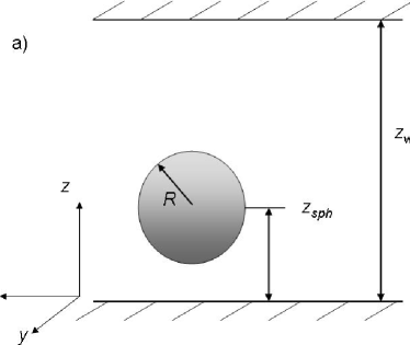
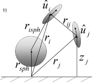
Figure 1: a) Schematic view of the system under consideration. b) The different interactions between the mesogens and the colloid.

The system considered in this work comprises 11460 liquid crystal particles confined between two soft repulsive walls at $z=0$ and $z=Z_{\text{wall}}$ (see Figure 1a). Simulations were conducted at a constant temperature $T^{*}=1.0$ and an average number density of $\rho^{*}=0.335$. All variables are given in reduced units, e.g. $\rho^{*}=N\sigma_{0}^{3}/V$, $T^{*}=kT/\epsilon_{0}$, where $\sigma_{0}$ and $\epsilon_{0}$ are length and energy parameters which are set to unity. The shape of the simulation box is orthorhombic; the side lengths are equal in the $x$ and $y$ directions. Periodic boundary conditions apply in $x$ and $y$. Mesogens $i$ and $j$ interact via a shifted and truncated Gay–Berne (GB) potential gay81 :

$$U_{ij} = \begin{cases}4\epsilon_{0}(\varrho_{ij}^{-12}-\varrho_{ij}^{-6})+\epsilon_{0},\quad&\varrho_{ij}^{6}<2\\ 0,\quad&\varrho_{ij}^{6}>2\end{cases}$$ (12)

$$\varrho_{ij} = (|\bm{r}_{ij}|-\sigma_{ij}+\sigma_{0})/\sigma_{0}$$ (13)

$$\sigma_{ij} = \sigma_{o}\left[1-\frac{\chi}{2}\left\{\frac{\left(\hat{\bm{r}}_{ij}\cdot\hat{\bm{u}}_{i}+\hat{\bm{r}}_{ij}\cdot\hat{\bm{u}}_{j}\right)^{2}}{1+\chi\hat{\bm{u}}_{i}\hat{\bm{u}}_{j}}+\frac{\left(\hat{\bm{r}}_{ij}\cdot\hat{\bm{u}}_{i}+\hat{\bm{r}}_{ij}\cdot\hat{\bm{u}}_{j}\right)^{2}}{1-\chi\hat{\bm{u}}_{i}\hat{\bm{u}}_{j}}\right\}\right]^{-1/2}$$ (14)

$$\chi = \frac{\kappa^{2}-1}{\kappa^{2}+1}.$$ (15)

where $\hat{\bm{u}}_{i}$ and $\bm{r}_{ij}$ denote molecular orientations (along the main axis of the ellipsoid) and intermolecular vectors ($\bm{r}_{ij}=\bm{r}_{i}-\bm{r}_{j}$, where $\bm{r}_{i}$ is the position of particle $i$); unit vectors are identified by hats ($\hat{\bm{r}}_{ij}=\bm{r}_{ij}/|\bm{r}_{ij}|$). For details see Figure 1b. Parameter $\kappa=3$ in this work is the length to width ($\sigma_{0}$) ratio. The interactions of a GB mesogen $i$ with all interfaces are described by the same potential (12), where the $\varrho_{ij}$ are defined as follows for a sphere and a surface:

$$\varrho_{i\text{sph}} = \left(|\bm{r}_{i}-\bm{r}_{\text{sph}}|-{R}+\sigma_{0}/2\right)/\sigma_{0},$$ (16)

$$\varrho_{i\text{wall}} = \left(|\bm{z}_{i}|+\sigma_{o}/2\right)/\sigma_{0}.$$ (17)

In this case, $\bm{r}_{\text{sph}}$, $\bm{r}_{i}$, and $|\bm{z}_{i}|$ denote the position vectors for the centers of mass of the sphere, mesogen $i$, and the normal distance from a surface, respectively; $R$ represents the radius of the sphere. This potential has been employed in a previous study of a colloidal particle in a bulk liquid crystal andrienko01 , and is known to reproduce topological defects around the particle that are in agreement with theory and experiment. The force on a sphere is calculated as the derivative of the interaction potential between the liquid crystal and the sphere with respect to $z$; due to symmetry in the $(x,y)$-plane, only the $z$-component of the force contributes. The surface and sphere interact as hard bodies, i.e. the minimum distance possible between a surface and the center of mass of the sphere is the radius of the sphere, which is set to 3.

Before proceeding with this system, we characterized the confined Gay-Berne system without a colloid in independent simulations. The separation between the walls was chosen to be $Z_{\text{wall}}=34$. A second rank order parameter $P_{2}$ is defined as

$$P_{2}=\frac{1}{2}\langle 3(\hat{\bm{u}}_{i}\hat{\bm{P}})^{2}-1\rangle,$$ (18)

where $\hat{\bm{P}}$ is the average orientation of the system. Figure 2 shows the resulting profiles of density and order parameter. One can see that several layers are formed at the surface. In the midsection between the walls both density and $P_{2}$ profiles are almost flat. In that midsection, a sphere is unlikely to “feel” the presence of a substrate. On the other hand, the movement of the sphere in the vicinity of the surface may be severely limited or dictated by the layered structure of the liquid crystals.

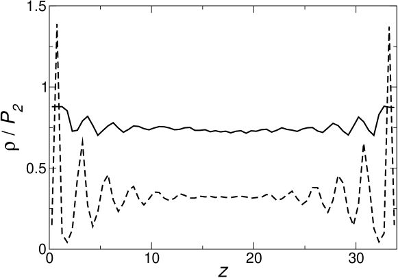
Figure 2: Density (dashed line) and $P_{2}$ (solid line) profiles for a confined system.

IV Results and Discussion

The quantity of interest is the free energy profile for a colloidal sphere in a confined nematic liquid crystal as a function of distance between the center of mass of the sphere and the surface. From the results shown in Figure 2 the fluid structure is rich near the surface and bulk-like for $z>13$. Hence, we concentrate on the region $3\leq z_{\text{sph}}\leq 13$, where $z_{\text{sph}}$ denotes the position of the center of mass of a sphere and plays the role of a reaction coordinate. The lower bound is the radius of the sphere. As a first trial, $NVT$ MC simulations were performed with $z_{\text{sph}}$ fixed at specific values. A plot

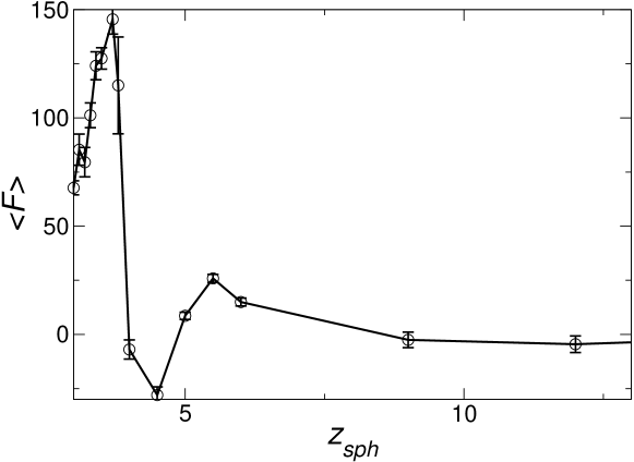
Figure 3: Mean force acting on a colloidal sphere from a standard Monte Carlo calculation.

(Figure 3) of the mean force acting on a sphere from these calculations indicates that indeed the effective force from the wall on a sphere is increasingly repulsive (positive) up to $z_{\text{sph}}=3.8$ and then decreases to zero around the value of 4. The force then changes from repulsive to attractive and back to repulsive and becomes seemingly constant and neutral for $z_{\text{sph}}>9$. From the graph we can infer that at $z_{\text{sph}}=4$ the system reaches a stable equilibrium. This is confirmed by simulations of a freely moving sphere; from its original position of $z_{\text{sph}}=3$, the sphere travels within a few MC cycles to a position of $z_{\text{sph}}=4$, where it undergoes only slight oscillations. The structure of the liquid crystals near the surface influences considerably the mean force on a sphere, but conventional $NVT$ Monte Carlo simulations are unable to elucidate the details of these interactions.

Next, we performed umbrella sampling simulations for $z_{\text{sph}}$ near the surface. In that region, the energy profile was found to vary strongly. Highly stiff springs are necessary, which in turn result in very narrow windows. To widen the range of the windows and improve their overlap, we applied spring potentials of the form $U_{\text{umb}}=A(z_{\text{sph}}-z_{0})^{4}+B(z_{\text{sph}}-z_{0})^{2}$, where $z_{0}$ is an equilibrium position for a spring and $A>0$ and $B<0$. Such potentials have a “W” shape and therefore result in a slight dispersion of a sphere close to $z_{0}$. Depending on the behavior of the system, at some points we had to use hybrid springs that combined a stiff harmonic spring on one side of $z_{0}$ and a dispersing potential on the other. As a result, 13 windows were necessary to explore the narrow range of $z$ between $[3.0,4.2]$. The corresponding umbrella potentials are given in Table 1.

No	$A$	$B$	$z_{0}$
1	0	750	3.0
2∗	240 000	$-1\,200$	3.15
2′	0	25 000	3.15
3∗	240 000	$-1\,200$	3.2
3′	0	3 750	3.2
4	320 000	$-1\,600$	3.2
5	50 000	$-1\,000$	3.2
6	9 877	$-444$	3.2
7	3 125	$-250$	3.2
8	292 969	$-938$	3.5
9	15 802	$-178$	3.5
10	0	50 000	3.7
11	2 858	$-185$	3.5
12∗	320 000	$-1600$	3.9
12′	0	25 000	3.9
13	16	$-18$	4.0

Table 1: Values for the umbrella potentials $U_{\text{umb}}=A(z_{\text{sph}}-z_{0})^{4}+B(z_{\text{sph}}-z_{0})^{2}$. Potentials marked with an asterisk are only applied to the left hand side of $z_{0}$, potentials marked with a prime are only applied to the right hand side of $z_{0}$.

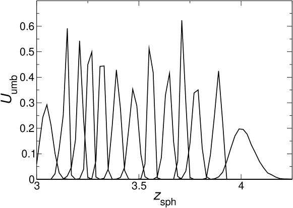
Figure 4: Energy histograms from umbrella sampling simulations for 13 independently simulated umbrella potentials or windows.

Figure 4 shows corresponding histograms collected over a simulation of $3$–$5\times 10^{5}$ MC cycles from the initially equilibrated configurations. Not surprisingly, a histogram centered at 4 is wide and Gaussian in appearance, whereas the others are sharp and narrow. Histogram data $g_{i}(z_{\text{sph}})$ are transformed by taking the natural logarithm and subtracting the corresponding umbrella potentials. Even though each data set is offset by a constant, there appear to be at least two separate regions where different functions must be fitted. We fit the first 12 sets and the last set separately using third degree polynomials by a least squares procedure modified to include constant offsets (see Figure 5); the third degree was chosen as the minimum required to have an inflection point, i.e. the derivative of the force is zero. The intersection of forces (negative derivatives) is taken as the matching point; the curves of the potential of mean force are joined at that point $(z_{\text{sph}}=3.8,F(z_{\text{sph}}=3.8)=164)$ setting the PMF at $z_{\text{sph}}=3$ to zero. The resulting force profile (see Fig. 6) is in agreement with results of canonical simulations but reveals more detail.

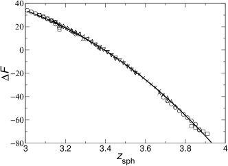
Figure 5: Left: original Boltzmann inverted histograms from umbrella sampling simulations. Right: The histograms of the 12 lower windows collapse onto a master plot to yield an effective relative free energy as a function of the distance of the colloid from one of the walls (see text).

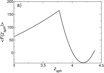
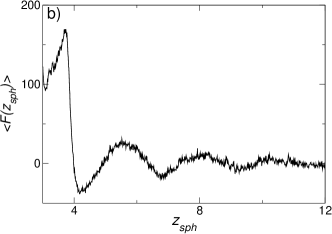
Figure 6: The mean force acting on the sphere calculated by the umbrella simulation technique (a) and from the novel technique (b)

Next, the application of the new method is demonstrated on the same system. A state $m$ is defined by the position of the center of mass of a sphere in the range $(m-1)\Delta z<z_{\text{sph},m}\leq m\Delta z$. The entire range of $[3,13]$ is divided into nine overlapping windows of width 2: the first window covers $3\leq z_{\text{sph}}<5$, the second window covers $4\leq z_{\text{sph}}<6$, etc. Each window consists of 200 states with $\Delta z=0.01$. A move to a new state, i.e. a move of a sphere in the $z$ direction (its $x$ and $y$ coordinates are kept at zero throughout the entire simulation) is attempted every Monte Carlo cycle; a cycle consists of a trial displacement or rotation of all liquid crystal particles. Initially, all weighting factors $g_{m}$ and the convergence factor $f$ are given a value of $e^{0.1}$. Simulations proceed for three DSMC cycles: that is, $\ln f$ is halved twice. The resulting mean force and relative weights are averaged between windows in the area of overlap. Figure 6b shows the results for the mean force. The corresponding free energy profiles are shown in Figure 7 (integrated mean force; PMF was arbitrarily set to 0 at $z_{\text{sph}}=3)$. It is evident from the above plots that the EDOS method provides improved sampling compared to simple $NVT$ or umbrella potential simulations. Moreover, more details of the interaction of the colloidal sphere with the liquid crystals and the surface are visible (compare Figures 3 and 6a). Note that with only 9 windows it is possible to cover a substantially wider range than with 13 windows in umbrella sampling.

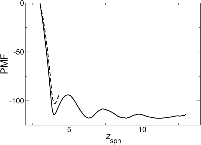
Figure 7: The potential of mean force between the the sphere and the surface calculated by the novel technique (solid line). For comparison the umbrella calculated PMF is also shown (dashed line).

It is apparent that the mean force on the sphere has different characteristics in various regions in proximity of the surface. Close to the surface, the force is strongly repulsive and reaches its maximum ($F_{max}\approx 170$) at $z_{\text{sph}}\approx 3.8$. The force then decreases rapidly, dropping to zero at $z_{\text{sph}}=4$ and eventually reaching a minimum $(F_{min}\approx-35)$ at $z_{\text{sph}}=4.3$. In the interval $4<z_{\text{sph}}<11$ the force exhibits a damped oscillatory behavior with a wavelength of about 2.5–2.6. The force oscillations die out within about 2–3 of these wavelengths. At that point ($z_{\text{sph}}\approx 11$) the force becomes effectively zero.

Clearly, the layered structure of the liquid crystals has a strong effect on the behavior of a suspended colloidal sphere. The effect appears to be most pronounced in the immediate vicinity of the surface, where the density and the order parameter are comparable to those of a smectic or even solid layer. Figure 8 shows pictures of the colloid seen from below (the surface was removed for clarity). The sphere severely disrupts the first, dense layer of liquid crystals; as the sphere moves away from the surface, the cavity caused by it gradually fills up. At $z_{\text{sph}}=3.8$ the layer is almost completely restored. At $z_{\text{sph}}=4$, the first layer is fully repaired; this point corresponds to a stable state of the system as the force on the sphere vanishes (see above).

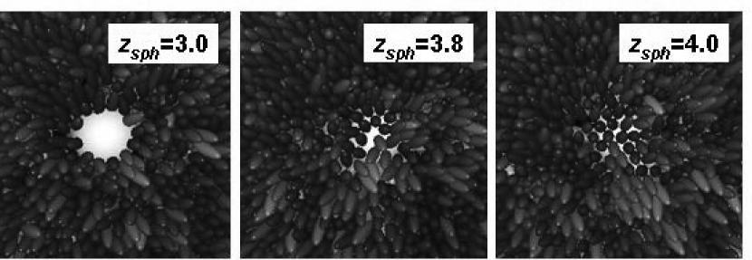
Figure 8: Views through the surface onto the sphere for $z_{\text{sph}}=3,3.8,4$ (left to right)

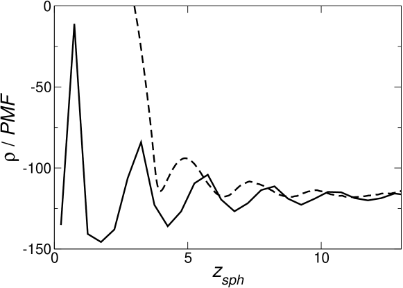
Figure 9: Density of the confined system without the sphere (solid line) overlaid with the potential of mean force gained by the novel method (dashed line). The density was scaled and shifted along $y$-axis arbitrarily.

As for subsequent undulations in the force profile, their wavelength approximately coincides with the thickness of the liquid crystalline layers close to the surface. If we superimpose the density profile of the confined system without the sphere (see Figure 9) onto the PMF curve, the oscillations are almost in phase. The PMF curve is slightly shifted to larger distances from the surface (offset in $z_{\text{sph}}\approx 0.25)$. The minima in the PMF practically match those of the density profile; our results indicate that the sphere prefers to reside between adjacent LC layers.

V Conclusion

A new method is proposed in which a density of states Monte Carlo formalism is used to self-consistently calculate the weights for an expanded ensemble technique. This method permits efficient calculation of the potential of mean force of a complex system. Its application is illustrated in the context of a colloidal sphere dispersed in a confined nematic host.

The method allows one to determine with high resolution the mean force on the colloid as a function of its separation from the surface; the results agree qualitatively with less efficient methods such as umbrella sampling and conventional canonical Monte Carlo. Clearly, the layered structure of the liquid crystals near the surface profoundly influences the mean force on the colloid. The snapshots of the system at several distances indicate that the disruption of the first surface layer is most likely responsible for the strong repulsive force very close to the surface. Once the “hole” caused by the sphere is completely filled in, the force decreases to neutral at $z_{\text{sph}}=4$, resulting in a preferred position for the colloid reflected by a minimum in its free energy (potential of mean force). At larger distances, both the force and the potential of mean force profiles display undulations that are almost in phase with the oscillations in the density profile of the confined system. It is worth pointing out again that all intermolecular interactions in the simulation are strictly repulsive. The attractive regions in the potential of mean force between the colloid and the surface have therefore purely entropic origins. Additional studies are currently under way to elucidate the nature of the interaction between the surface and the colloid for different sphere sizes and different ancoring conditions.

References

- (1) V. K. Gupta, J. J. Skaife, T. B. Dubrovsky, and N. L. Abbott, Science 279, 2077 (1998).
- (2) J. A. Van Nelson, S.-R. Kim, and N. L. Abbott, Langmuir 18, ASAP article (2002).
- (3) P. Poulin, H. Stark, T. C. Lubensky, and D. A. Weitz, Science 275, 1770 (1997).
- (4) P. Poulin and D. A. Weitz, Phys Rev E 57, 626 (1998).
- (5) Y. Gu and N. L. Abbott, Phys Rev Lett 85, 4719 (2000).
- (6) J. L. Billeter and R. A. Pelcovits, Phys Rev E 62, 711 (2000).
- (7) D. Andrienko, G. Germano, and M. P. Allen, Phys Rev E 63, 041701 (2001).
- (8) B. Roux, Comput Phys Commun 91, 275 (1995).
- (9) O. Engkvist and G. Karlström, Chem Phys 213, 63 (1996).
- (10) J. VandeVondele and U. Röthlisberger, J Chem Phys 113, 4863 (2000).
- (11) T. P. Straatsma, M. Zacharias, and J. A. McCammon, Chem Phys Lett 196, 297 (1992).
- (12) M. Sprik and G. Ciccotti, J. Chem. Phys. 109, 7737 (1998).
- (13) F. Wang and D. P. Landau, Phys. Rev. Lett. 86, 2050 (2001).
- (14) P. M. C. de Oliveira, T. J. P. Penna, and H. J. Herrmann, Braz. J. Phys. 26, 277 (1996).
- (15) D. Chandler, Introduction to Modern Statistical Mechanics, Oxford University Press, New York, 1987.
- (16) G. M. Torrie and J. P. Valleau, Chem. Phys. Lett. 28, 578 (1974).
- (17) T. C. Beutler and W. F. Van Gunsteren, J Chem Phys 100, 1492 (1994).
- (18) B. A. Berg and T. Neuhaus, Phys. Rev. Lett. 68, 9 (1992).
- (19) A. M. Ferrenberg and R. H. Swendsen, Phys. Rev. Lett. 61, 2635 (1988).
- (20) A. P. Lyubartsev, A. A. Martinovski, S. V. Shevkunov, and P. N. Vorontsov-Velyaminov, J. Chem. Phys. 96, 1776 (1992).
- (21) F. A. Escobedo and J. J. de Pablo, J Chem Phys 103, 2703 (1995).
- (22) F. Wang and D. P. Landau, Phys Rev E 64, 056101 (2001).
- (23) Q. Yan, R. Faller, and J. J. de Pablo, J Chem Phys 116, 8745 (2002).
- (24) R. Faller and J. J. de Pablo, Direct calculation of the density of states of a binary lennard-jones glass, submitted.
- (25) N. Rathore and J. J. de Pablo, J Chem Phys 116, 7225 (2002).
- (26) T. S. Jain and J. J. de Pablo, J Chem Phys 116, 7238 (2002).
- (27) E. B. Kim, R. Faller, and J. J. de Pablo, Estimation of the chemical potential of liquid crytal molecules by simulation, in preparation.
- (28) R. Faller, Q. Yan, and J. J. de Pablo, J Chem Phys 116, 5419 (2002).
- (29) J. G. Gay and B. J. Berne, J Chem Phys 74, 3316 (1981).