On the Aizenman exponent in critical percolation

Abstract

The probabilities of clusters spanning a hypercube of dimensions two to seven along one axis of a percolation system under criticality were investigated numerically. We used a modified Hoshen–Kopelman algorithm combined with Grassberger’s “go with the winner” strategy for the site percolation. We carried out a finite-size analysis of the data and found that the probabilities confirm the Aizenman’s proposal of the multiplicity exponent for dimensions three to five. A crossover to the mean-field behavior around the upper critical dimension is also discussed.

Percolation occurs in many natural processes, from electrical conduction in disordered matter to oil extraction from field. In the latter, the coefficient of oil extraction from oil sands (the ratio of the actually extracted to the estimated oil) can be as much as 0.7 for light oil and as low as 0.05 for viscous heavy oil. An increase in this coefficient by any new point requires appreciable investment. Additional knowledge about the percolation model could reduce the amount of additional investment.

A remarkable breakthrough in the theory of critical percolation was established in the last decade thanks to a combination of mathematical proofs, exact solutions, and large-scale numerical simulations. Recently, Aizenman has proposed a new exponent that describs the probability $P(k,r)$ of a critical percolation $d$-dimensional system with the aspect ratio $r$ being spanned by at least $k$ clusters Aiz97 ,

$$\ln P(k,r)\propto-\alpha_{d}\;k^{\zeta}\;r,$$ (1)

where $\alpha_{d}$ is a universal coefficient depending only on the universality class, and $\zeta=d/(d-1)$.

In two dimensions, Aizenman’s proposal (1) was proved mathematically Aiz97 , confirmed numerically SK1 , and derived exactly Cardy98 using conformal field theory and Coulomb gas arguments. This exponent seems to be related to the exponents of two-dimensional copolymers Dup . In three dimensions, proposal (1) was checked numerically in Lev99 and, more recently and more precisely, in Grass02 .

The upper critical dimension of percolation is $d_{c}=6$, which follows from the comparison of the exponents derived on the Cayley tree with those satisfying scaling laws (see, e.g., StAh and BH ). The fractal dimension $D_{f}$ of percolating critical clusters is equal to 4 above $d_{c}$, and the number of percolating clusters becomes infinite for $d>d_{c}$. This fact would imply that $\zeta=0$ at $d=6$ if we supposed (rather naively) that Aizenman’s formula applies at the upper critical dimension. Supposing that this is true and taking into account that the values of $\zeta$ for $d=2$ and $d=3$ are, respectively, $2$ and $1.5$, we can place all three points on the straight line $\zeta=(6-d)/2$, as depicted in Fig. 1. We can then estimate the respective values of $\zeta$ for $d=4$ and $d=5$ to be $\zeta=1$ and $\zeta=0.5$; these values are far from those predicted by Aizenman’s formula giving $4/3$ and $5/4$, respectively. In contrast, based on simulations, Sen Sen97 claims that $\zeta=2$ for all dimensions from two to five.

Figure 1: Variation of Aizenman exponent $\zeta$ with the space dimension $d$ as predicted by Aizenman (circles and dotted line), claimed by Sen (dashed line) and discussed in the text (solid line).

The main purpose of our simulations is to estimate the exponents for the dimensions from two to six with an accuracy sufficient for distinguishing between the values predicted for $d=4$ and $d=5$ by the Aizenman’s formula and a naive application of cluster fractal-dimension arguments and by the straight-line fit, as discussed above.

In the rest of the paper, we briefly summarize the highlights of our study, then present some details of our research, and finally discuss the results for the Aizenman exponent and the physics of a crossover from the Aizenman picture to the mean-field picture.

Our main results can be summarized as follows:

1. Modified combination of the Hoshen–Kopelman algorithm and Grassberger’s strategy. We use the Hoshen–Kopelman (HK) algorithm HK to generate clusters and Grassberger’s “go with the winner” strategy Grass02 to track spanning clusters. We add a new tag array in the HK algorithm, which allows the reduction of the tag memory order from $L^{d}$ to $L^{d-1}$, where $L$ is the linear size of the hypercubic lattice. As a result, the amount of memory is about two orders less for large values of $L$, and the program is about four times faster—the complexity of the algorithm is compensated by the lower memory capacity needed for for swapping to and from the auxiliary array.

2. Efficient realization of combined shift-register random number generators. We use an exclusive-or ($\oplus$) combination $z_{n}$ of two shift registers:

$$x_{n} = x_{n-9689}\oplus x_{n-5502},$$

$$y_{n} = y_{n-4423}\oplus y_{n-2325},\qquad z_{n}=x_{n}\oplus y_{n}$$ (2)

(see RNG and the references therein). We reduce the computational time for generating random numbers by a factor 3.5 through an efficient technical modification: we use the SSE command set that is available on processors of the Intel and AMD series starting from the Intel Pentium III and AMD Athlon XP.

3. Extraction of the exponents for dimensions three to five. We first use finite-size analysis to estimate the logarithm of the probability $P(k,r)$ in the limit of infinite lattice size $L$. We then fit data as a function of the number of spanning clusters $k$ to obtain the Aizenman exponent $\zeta$.

4. Confirmation of Aizenman’s proposal. The estimates of the exponent $\zeta$ for the dimensions $d=2,3,4$, and $5$ coincide well with those proposed by Aizenman.

5. Qualitative interpretation of Aizenman’s conjecture. Cardy interpreted Aizenman’s result qualitatively in two dimensions on the basis of assumption that the main mechanism for reducing the number of percolation clusters is that some of them terminate. The same result can be derived for the cluster confluence (or merging) mechanism. This means that, in low dimensions, the percolation clusters consist of a number of closed paths (loops), while, in higher dimensions, clusters are more similar to trees. Indeed, it is well known that the probability of obtaining loop becomes lower for higher dimensions and goes to zero in the limit of infinite dimensions (Cayley tree) StAh ; BH .

6. Crossover to mean-field behavior. We found evidence that the probability of clusters spanning a hypercubic lattice tends to unity in the limit of high dimensions, as it follows from the well-accepted picture. We did not find any dramatic changes in the probabilities around the upper critical dimension $d_{c}=6$, but rather found evidence for a crossover. Therefore, Aizenman’s formula (1) can also apply to dimensions higher (but not too much higher) than the upper critical dimension and describe approximately the probabilities of spanning clusters in large, though finite-size systems.

We follow with the details of the critical percolation, simulations, and data analysis.

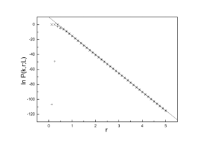
Figure 2: The logarithms of the probabilities of exactly $k$ clusters $P(k,r;L)$ ($+$) and of at least $k$ clusters $P_{+}(k,r;L)$ ($\times$) for the dimension $d=4$ and the number of clusters $k=5$ as functions of the aspect ratio $r$. The linear size of the hyperrectangle is $L=16$. The solid line is the linear approximation to $\ln P(k,r;L)$ on the interval $r=[1.5;5.0]$.

Spanning probability.

We can define the probability $P(k,r;L)$ that $k$ clusters traverse a $d$-dimensional hyperrectangle $[0,L]^{d-1}\times[0,Lr]$ in the $Lr$ direction Aiz97 . Provided that the scaling limit exists (this was proved recently by Smirnov for the percolation in plane Smirnov ), the probability $P(k,r)$ can be defined as the limit of $P(k,r;L)$ as $L\to\infty$. Aizenman proposed that $P(k,r)$ should behave according to (1) in dimensions from three to five. The validity of formula (1) for the percolation in plane was well established in Aiz97 ; Cardy98 ; SK1 .

Numerical results (Lev99 and Grass02 ) for the exponent $\zeta$ for critical percolation on cubic lattices seems to confirm Aizenman’s proposal for the value of $\zeta=1.5$

Actually, we could consider the probability $P(k,r)$ as the probability of obtaining $k$ clusters at the distance $r$ from the left side of the hyperrectangle if clusters grow to the right. Only two processes can change the number of clusters: cluster merging and cluster terminating.

The differential $dP$ of the probability is

$$dP\propto P(k,r)\;k^{1/(d-1)}\;k\;dr,$$ (3)

where the right-hand side represents the product of the probability $P(k,r)$ and the differential of the total border hyperarea of $k$ clusters, each with the hyperarea differential $k^{1/(d-1)}\;dr$. This expression follows from the fact that area unit of measure is proportional to the characteristic transverse length of “infinite” clusters. Therefore, the transverse area remains constant as $k$ changes, while the longitudinal length increment in these units is $\propto k^{1/(d-1)}dr$. Integrating (3), we recover probability (1). Thus, $P(k,r)$ describes the probability that $k$ clusters do not merge together.

The same probability could be obtained by the process of cluster termination, as given by Cardy in plane Cardy98 , which can easily be extended to dimensions $d>2$.

This means that the exponent $\zeta$ cannot be larger than the one proposed by Aizenman, and $\zeta=d/(d-1)$ is the upper bound for the exponent.

d	k	$L_{min}$	$L_{max}$	$\delta L$	$\qquad p_{c}$	Ref.
2	1-5	16	256	16-32	0.59274621(13)	pc2
3	1-6	8	64	4,8	0.3116080(4)	pc3
4	1-6	8	48-56	4,8	0.196889(3)	pc45
5	1-6	4	32,24	4,8	0.14081(1)	pc45
6	1-6	4	15-16	3-5	0.109017(2)	pc6
7	1-4	4	10	1	0.0889511(9)	pc6

Table 1: Minimal $L_{min}$ and maximal $L_{max}$ linear sizes of the percolation lattice and the interval $\delta L$ between two consecutive values of $L$ depending on the dimension $d$ and number of clusters $k$. The values of $p_{c}$ are taken from the references in the last column.

Algorithms and realizations.

The classical realization of the HK algorithm HK requires memory for two major structures: an array for keeping a $(d{-}1)$-dimensional cluster slice and a tag array. The total memory required by the algorithm is $\propto L^{d-1}+p_{c}rL^{d}$, where $p_{c}$ is the site percolation threshold value. Therefore, for large $rL$, one of the main advantages of the HK algorithm (i.e., relatively low memory consumption) is negated by the second term. Our modification of the original algorithm allows the memory for the tag array to be reduced to about $3p_{c}L^{d-1}$.

Instead of keeping all tags in memory and selecting new tags with increasing tag numbers, we create two arrays, of which one keeps the tag value and the other one keeps the number $N$ of the slice where the corresponding tag was last used. When we build a cluster, we update this array with $N=N_{\mathrm{current}}$ for the tags used. If $N<N_{\mathrm{current}}-1$, then this tag is not on the front surface of the sample, and it will never be used again so that we can, therefore, reuse it. We note that cluster size information should be taken into account before reusing the associated tag, if the size information is required.

We use the “go with the winner” strategy Grass02 as follows. If the system has $k$ spanning clusters for some aspect ratio $r=n\mathit{\delta r}$, it is stored in memory and is grown for $\mathit{\delta r}$. If the resulting configuration has $k$ spanning clusters, it is stored, and the growth process continues. Otherwise, we return to the previously saved state. Using this procedure, we calculate the probability $P_{i}(\mathit{\delta r})$ that the system propagates at the distance $\mathit{\delta r}$ from the position $r=(i-1)\mathit{\delta r}$. Finally, we obtain $P(r=n\mathit{\delta r})=\prod_{i=1}^{n}P_{i}(\mathit{\delta r})$. By choosing sufficiently small values of $\mathit{\delta r}$, we can achieve rather high probabilities of $P_{i}(\mathit{\delta r})$ (which can be determined from a few realizations), while the total probability may be very small (down to $\propto 10^{-100}$ in our case).

The random number generator was optimized for the SSE instruction set as follows. Because the length of all four RNG legs is $\{a|b\}_{\{x|y\}}>4$, the $n$th step of the RNG does not intersect with the ($n{+}3$)th step. Therefore, we can pack four consecutive 32-bit values of {$x_{n-\{a_{x}|b_{x}\}}$} and {$y_{n-\{a_{y}|b_{y}\}}$} into 128-bit XMM registers, process them simultaneously (see Eq. (2)), and thus obtain $z_{n}$, $z_{n+1}$, $z_{n+2}$, and $z_{n+3}$ within one RNG cycle.

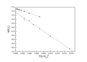
Figure 3: Plot of $s(k;l)$ for $k=3$ clusters in the dimension four as a function of $1/(L+L_{0})$ with the fitting parameter $L_{0}=4.12$ ($\square$) and for $k=4$ clusters in the dimension six with $L_{0}=4.03$ ($\diamond$). Straight lines result from the fitting to the corresponding data as discussed in the text.

Data analysis.

The lattice size was varied from $L_{min}$ to $L_{max}$ with the step $\delta L$. In Table 1, particular values of the simulation parameters are presented together with the interval of the number of clusters $k$ depending on the dimension $d$. The direct result of the simulations is the probabilities $P(k,r;L)$ that exactly $k$ clusters connect two opposite surfaces (separated by the distance $rL$) of the rectangle with size $L^{d-1}$ in the “perpendicular” direction in which we apply periodic boundary conditions. We use the values of the site percolation thresholds on hypercubic lattices from pc2 –pc6 , as shown in Table 1.

	d
$k$	3	4	5	6	7
1	-1.377(1)	-1.774(3)	-1.859(9)	-1.76(2)	-1.48(4)
2	-6.919(6)	-6.330(15)	-5.57(6)	-4.73(8)	-3.55(11)
3	-13.655(15)	-11.64(4)	-9.95(12)	-8.27(12)	-6.25(16)
4	-21.47(3)	-17.77(6)	-14.65(20)	-11.95(25)	-9.3(3)
5	-30.23(3)	-24.02(8)	-19.9(3)	-15.75(30)
6	-40.02(6)	-31.0(1)	-25.0(3)	-22.7(2)

Table 2: Values of $s(k)$ for different numbers of clusters $k$ and dimensions $d$ for site percolation on hypercubic lattices with periodic boundary conditions in directions perpendicular to the spanning direction.

Data analysis consists of three steps. First, we compute the slope $s(L)$ of $\ln P(k,r;L)$ for a given dimension $d$, number of clusters $k$, and linear lattice size $L$. An example of such a function is given in Fig. 2 for $\ln P(5,r;16)$ in the dimension four. We also plot the logarithm of the probability $P_{+}(k,r;L)=\sum_{k^{\prime}\geqslant k}P(k^{\prime},r;L)$ of the event that, at least, $k$ clusters span the (hyper)rectangle at the distance $rL$. To calculate $s(L)$, we use data only in the interval of the aspect ratio $r$ between $1.5$ and $5$. We note that the probability of five clusters spanning a rectangle with the linear size $L=16$ at the distance $5\cdot 16=80$ is extremely small $\approx 10^{-52}$.

Second, we compute probabilities in the limit of an infinite system size $L$, fitting slopes $s(k)$ with the expression (see Fig. 3)

$$s(k;L)=s(k)+\frac{B}{(L+L_{0})^{t}},$$ (4)

where $B$, $t$, and $L_{0}$ are fitting parameters Ziff92 ; Lev99 ; Ziff02 . The resulting values of the slopes $s(k)$ are presented in Table 2. The number of runs used to compute each particular entry in Table 2 varied from $10^{6}$ to several tens for higher dimensions.

$k$	this paper	exact from Cardy98	from Lev99
1	-0.6541(5)	-0.6544985	-0.65448(5)
2	-7.855(3)	-7.85390	-7.852(1)
3	-18.32(1)	-18.3260	-18.11(15)
4	-32.99(3)	-32.9867
5	-51.83(2)	-51.8363

Table 3: Values of $s(k)$ in two dimensions for different $k$ calculated in this paper, using the exact Cardy formula Cardy98 , and estimated in Lev99 for site percolation on a tube.

We checked the accuracy of our simulations, as well as the validity of the approach in general for site percolation on a square lattice. Table 3 shows a comparison of our results for the slope $s$ with the exact values and with earlier simulations, in which the other modification of the HK algorithm, but not the Grassberger strategy, was used. We note that our results coincide well with the exact results and give a higher accuracy for larger values of $k$ in comparison with the previous numerical results, despite the smaller computation time used. Our data for $k=1$ is less accurate because of the smaller statistics ($10^{6}$ runs, compared to $10^{8}$ samples in Lev99 ). This is a direct demonstration of the effectiveness of the Grassberger strategy for large values of $k$.

Finally, we use values in Table 2 to determine the Aizenman exponent $\zeta$ by fitting data in each column to

$$s=A(k^{2}-k_{0})^{p/2}$$ (5)

in two and three dimensions, as proposed by Grassberger Grass02 , and to

$$s=A(k^{p}-k_{0})$$ (6)

in higher dimensions. Here, $A$, $k_{0}$, and $p$ are fitting parameters. We take only the leading behavior in $k$ into account.

$d$	$\quad A$	$\quad k_{0}$	$\quad p$
2	2.090(4)	0.244(5)	2.0012(10)
	2.0940(5)	0.2489(7)	2
3	2.81(4)	0.64(4)	1.489(7)
	2.757(2)	0.587(3)	3/2
4	3.06(20)	0.41(6)	1.315(30)
	2.949(5)	0.373(3)	4/3
5	2.8(1)	0.40(4)	1.24(3)
	2.78(2)	0.38(2)	5/4
6	2.8(8)	0.5(3)	1.12(14)
	2.41(5)	0.33(6)	6/5
7	1.4(10)	0.08(116)	1.4(4)
	2.03(12)	0.50(13)	7/6

Table 4: Values of the fitting parameters $A$ and $k_{0}$ and the power $p$ as defined in Eqs. (5) and (6) for the dimension $d$.

Spanning, proliferation, and crossover to mean-field behavior.

The results of the final fit to (5) and (6) are shown in Table 4. The second row for each particular dimension $d$ is the fit with the power $p$ fixed to the Aizenman exponent value. This is done to check the fit stability. Indeed, the values of $A$ and $k_{0}$ coincide within one standard deviation for the dimensions two to five.

The larger deviations of parameters for the dimensions six and seven may be attributed to appearance of cluster proliferation—the number of clusters is known Aiz97 to grow as $L^{d-6}$ in dimensions $d>d_{c}=6$. We plot the coefficient $\alpha_{d}$ (defined by expression (1)) in Fig. 4 as a function of the dimension $d$. The probability of exactly one cluster spanning at the given distance $r$ becomes smaller as the dimension increases from two to five and larger for larger dimensions, as can be seen from the first row ($k=1$) of Table 2 and from the lower curve dependence in Fig. 4. For any fixed $d$, the value of $\alpha_{d}$ approaches some limit for the dimensions two to five and $k>2$, which suggests the value of the corrections to the leading behavior in $k$ (see Eqs. (5) and (6)).

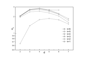
Figure 4: The coefficient $\alpha_{d}$ (as a function of the dimension $d$) extracted from the probabilities $P(k,r)$ for different numbers of clusters $k$.

The fact that the value of $\zeta$, which we formally extracted from our data for $d=6$, more or less coincides with $\zeta=d/(d-1)=6/5$, as formally calculated using the Aizenman expression, may be interpreted as an indication that the number of clusters depends logarithmically on the lattice size $L$. One can expect that the logarithmic behavior is visible only for somewhat larger values of $L$ than we have used so far (see Table 1). With the values of $L$ of the order we have used in simulations, we see effectively the same picture as for the lower dimensions—clusters spann according to the Aizenman formula. This means that at small (or moderate) values of $L$, the main mechanism is as discussed above: cluster merging and terminating. And only at sufficiently large system sizes we will see cluster proliferation. An indication of that can be seen from the values of $\alpha_{d}$ in the dimension seven in Fig. 4. The probabilities become closer, and this can be attributed to cluster proliferation and treated as a crossover to the mean-field behavior.

Discussion.

The results have shown the validity of the Aizenman’s proposal in the dimensions three to five (results on plane were already proved rigorously) and do not support Parongama Sen claims based on their simulations (Fig. 1). We have found evidence for cluster proliferation for the dimension seven. The analysis can be extended to the number of spanning clusters to distinguish exponential decay with the system size of the number of clusters for the dimension five, logarithmic growth of them for the dimension six, and linear growth for the dimension seven. The same technique can be used to establish numerically such a crossover to the mean-field picture, although a significantly longer computational time, than we used, is needed for this. In fact, the linear growth of the multiplicity of spanning clusters for seven-dimensional critical percolation was confirmed numerically in preprint ACF posted at arXiv preprint library a few days after our cond-mat/0207605.

- (1) M. Aizenman, Nucl. Phys. B 485 (1997) 551–582, cond-mat/9609240.
- (2) L.N. Shchur and S.S. Kosyakov, Int. J. Mod. Phys. C 8 (1997) 473–481, cond-mat/9702248.
- (3) J. Cardy, J. Phys. A, 31 (1998) L105, cond-mat/9705137.
- (4) B. Duplantier, Phys. Rev. Lett. 82 (1999) 880, cond-mat/9812439.
- (5) L.N. Shchur, in Computer Simulation Studies in Condensed-Matter Physics XII, eds. D.P. Landau, S.P. Lewis, and H.-B. Schüttler, (Springer-Verlag, Heidelberg, Berlin, 2000), cond-mat/9906013.
- (6) P. Grassberger, Comp. Phys. Comm., 147 (2002) 64, cond-mat/0201313; P. Grassberger and W. Nadler, cond-mat/0010265.
- (7) D. Stauffer and A. Aharony, Introduction to Percolation Theory (Taylor & Francis, London, 1992).
- (8) A. Bunde and S. Havlin, in Fractals and Disordered Systems, eds. A. Bunde and S. Havlin, 2nd Edition (Springer-Verlag, Berlin, 1996).
- (9) P. Sen, Int. J. Mod. Phys. C 8 (1997) 229, cond-mat/9704112.
- (10) J. Hoshen and R. Kopelman, Phys. Rev. B 14 (1976) 3438.
- (11) L.N. Shchur, Comp. Phys. Comm., 121-122 (1999) 83–85, hep-lat/0201015.
- (12) S. Smirnov, C.R. Acad. Sci. Paris 333 (2001) 239, www2.math.kth.se/stas/papers/percras.ps.
- (13) M.E.J. Newman and R.M. Ziff, Phys. Rev. Lett 85 (2000) 4104–4107, cond-mat/0005264.
- (14) C.D. Lorenz and R.M. Ziff, J. Phys. A 31 (1998) 8147, cond-mat/9806224.
- (15) G. Paul, R.M. Ziff, and H.E. Stanley, Phys. Rev. E. 64 (2001) 026115, cond-mat/0101136.
- (16) P. Grassberger, cond-mat/0202144.
- (17) R.M. Ziff, Phys. Rev. Lett. 69 (1992) 2670.
- (18) One could expect an increase in finite-size effects as increases. Indeed, this was found by R. Ziff (private communication) in two dimensions for large values of .
- (19) G. Andronico, A. Coniglio, S. Fortunato, hep-lat/0208009.