Magnetoplasmon Excitations and Spin Density Instabilities in an Integer Quantum Hall System with a Tilted Magnetic Field

Abstract

We study the magnetoplasmon collective mode excitations of integer quantum Hall systems in a parabolically confined quantum well nanostructure in the presence of a tilted magnetic field by using the time-dependent Hartree-Fock approximation. For even integer filling, we find that the dispersion of a spin density mode has a magneto-roton minimum at finite wavevectors, at a few times $10^{6}$ cm^-1 for parallel fields of order 1-10 Tesla, only in the direction perpendicular to the in-plane magnetic field, while the mode energy increases monotonously with wavevector parallel to the in-plane magnetic field. When the in-plane magnetic field is strong enough (well above 10 Tesla),we speculate that this roton minimum may reach zero energy, suggesting a possible second order phase transition to a state with broken translational and spin symmetries. We discuss the possibility for observing such parallel field-induced quantum phase transitions. We also derive an expression for the dielectric function within the time-dependent Hartree-Fock approximation and include screening effects in our magnetoplasmon calculation. We discuss several exotic symmetry-broken phases that may be stable in finite parallel fields, and propose that the transport anisotropy, observed recently in parallel field experiments, may be due to the formation of a skyrmion stripe phase predicted in our theory. Our predicted anisotropic finite wavevector suppression, perhaps even a mode-softening leading to the quantum phase transition to the anisotropic phase, in the collective spin excitation mode of the wide well system in the direction transverse to the applied parallel magnetic field should be directly experimentally observable via the inelastic light scattering spectroscopy.

I Introduction

Observations of integral quantum Hall effect (IQHE, 1980) and fractional quantum Hall effect (FQHE, 1982) are important landmarks of condensed matter physics in recent decades [1]. In quantum Hall systems, electrons are ”frozen” (in their orbital motion) in discrete Landau levels by the external magnetic field, and have gapped excitations at integer or fractional filling factors. There is considerable richness of the phase diagram when additional (i.e. in addition to the orbital motion) degrees of freedom associated with spin, layer, or subband index are introduced [1, 2, 3]. These multicomponent quantum Hall systems have been extensively studied both theoretically and experimentally in recent years. In general, since the spin (Zeeman) energy is much smaller than the cyclotron energy due to the small effective $g$-factor and the small effective mass of electrons in GaAs based QH systems, the spin degree of freedom is not important energetically compared to the orbital motion. But spin can be crucial when a second quantum Hall system is coupled coherently (for example, in a double quantum well [DQW] system) or an additional magnetic field is applied in the direction parallel to the two-dimensional (2D) semiconductor quantum well plane. In the first situation, the finite barrier energy between the two wells opens a gap ($\Delta_{SAS}$) between a symmetric and an antisymmetric subbands, which can be tuned by electron tunneling, layer separation, and/or bias voltage [2]. When $\Delta_{SAS}$ is close to the Zeeman splitting energy, interesting physics has been predicted theoretically [4] and observed experimentally [5, 6]. On the other hand, physics of the second situation, where a tilted magnetic field is applied to a wide width well (WWW) system to couple subbands of a wide well with spin-split Landau levels, has not yet been extensively explored. One reason for this is that the strength of the applied tilted magnetic field has to be very large ($>25$ Tesla) in order to sufficiently enhance the Zeeman energy to be comparable to the Landau level separation in GaAs. Such strong and uniform magnetic fields has only been available very recently [7]. From a theoretical point of view, studying QH effects in a WWW with tilted magnetic field is difficult because the in-plane magnetic field hybridizes the 2D electron subbands arising from the confinement potential in the growth direction (i.e. perpendicular to the 2D plane) with the orbital Landau levels so that the electron wavefunction of a WWW is a complicated combination of electric (“subbands”) and magnetic (“Landau levels”) quantization even at the single particle level. It is sometimes simplistically believed that, if parameters are chosen properly in an isospin language, then a WWW system in a tilted field (at least for) the closest two Landau levels near the degeneracy point could be approximately mapped onto a DQW system. We emphasize that this mapping is not exact and misses subtle and interesting physics associated with a WWW in a tilted field. For example, experimentally a WWW in a tilted field is found to display both three-dimensional (3D) and two-dimensional properties [8]. In some situations a WWW system could behave very much like a DQW system albeit with strong tunneling) [9]. More strikingly, the recent observation of anisotropic resistance at even filling factors in a WWW system with an in-plane field [7] shows a possible stripe phase formation induced by electron-electron interaction near a degeneracy or a level crossing point.

Inspired by the observed anisotropic transport properties at integer filling factors [7], we investigate in this paper the collective mode excitations of integer quantum Hall systems in a wide quantum well with a tilted magnetic field (i.e. in the presence of an in-plane magnetic field) by using the time-dependent Hartree-Fock approximation (TDHFA). We extend the work of Kallin and Halperin [10] for a strictly 2D system, i.e. a zero width well (ZWW) to a WWW system and derive a full analytical expression for the mode dispersion energy. To keep our theory analytically tractable we choose our quantum well confinement potential to be parabolic (”parabolic well”). Our choice of parabolic confinement is dictated by the fact that the corresponding single-particle problem (i.e. an electron moving in a one-dimensional parabolic potential along the $z$-direction in the presence of an arbitrary magnetic field) can be exactly analytically solved enabling essentially a complete analytic solution of the many-body TDHF solution of the collective mode spectra (essentially on the same footing as the 2D Kallin-Halperin work in Ref. [10]) in the WWW system in the presence of a tilted magnetic field (i.e. both the in-plane field and the perpendicular field producing the Landau quantization). The work presented in this paper is therefore a direct (and highly non-trivial) generalization of the strictly 2D Kallin-Halperin work [10] on the magnetoplasmons of a 2D electron gas (in the presence of only a perpendicular magnetic field) to a parabolic WWW system in the presence of a tilted magnetic field. We study both charge and spin mode collective excitations in systems of different electron densities, magnetic field strengths, and well widths. At even integer factors, we find that the dispersion of spin density mode has a magneto-roton minimum only at a finite wavevector in the direction perpendicular to the in-plane magnetic field, while it increases monotonously with respect to the wavevector parallel to the in-plane magnetic field. When the in-plane magnetic field is sufficiently strong, this roton minimum may reach zero energy before the ground state becomes polarized, suggesting a possible second order phase transition to a state with broken translational and spin symmetries. The possibility of this quantum phase transition (to an anisotropic symmetry-broken state) in the presence of a tilted field is one main new result of our work. We also derive the full formula for the dielectric function of the system within TDHFA by including the ladder diagrams consistently, so that it can be applied to other systems even when only few Landau levels are occupied. We include such screening in our collective mode calculation and discuss its effect to the magneto-roton minimum.

Before jumping into the details of the collective mode calculation, it is instructive to discuss in the appropriate context some earlier work in parabolic wells and in the ground state instability (i.e. the softening of collective modes) of similar systems. Among the models of finite width wells, parabolic wells are considered special, because the electron gas, in screening the parabolic conduction band edge potential, forms a constant density slab, being a good approximation to a 3D jellium where electrons move in a constant positive background charge density [11]. Furthermore, the parabolic confinement potential can be exactly diagonalized in a center-of-mass coordinate and therefore gives a non-spin-flip optical absorption energy exactly the same as its noninteracting result in the long wavelength limit (the so called generalized Kohn’s theorem) [12, 13]. As mentioned above,we use a parabolic confinement potential, because it allows us to find simple noninteracting eigenstates in the presence of a tilted magnetic field, which then provides a good starting point to consider many-body effects. The effects of imperfect parabolic confinement potential on the collective excitations have earlier been studied either with only a perpendicular magnetic field [14] or with only an in-plane magnetic field [15]. Only rather small quantitative corrections were found (for example, small shift of resonance energy, and slight broadening of the absorption peak) for realistic wells (which necessarily deviate from ideal parabolic confinement considered in our work). We believe, therefore, that our theoretical results should apply with quantitative accuracy to realistic parabolic quantum wells, and qualitatively to rectangular quantum wells [16].

It is generally believed that in both three and two dimensions, when an infinitely strong magnetic field is applied, electrons undergoes a phase transition to a Wigner crystal state with broken translational symmetry at low temperatures. In the intermediate magnetic field region, Celli and Mermin [17] proposed a long time ago a possible exchange induced spin-density-wave (SDW) instability in a three-dimensional electron system. More recently, GaAs based semiconductor wide parabolic wells have been proposed as good candidates for observing such SDW instabilities since wide parabolic wells are essentially ideal 3D electron systems [8, 18, 19]. Brey and Halperin [19] proposed that the SDW instability and the transport anisotropy should be observed in a wide parabolic semiconductor quantum well system when an intermediate in-plane magnetic field is applied. Similarly, correlation-driven intersubband SDW instability has been predicted by Das Sarma and Tamborenea in DQW systems at low carrier densities [20]. Intersubband-induced charge-density-wave (CDW) instability in a wide parabolic well with a perpendicular magnetic field was also investigated [21]. To the best of our knowledge, however, these theoretically proposed (translational symmetry breaking) instabilities have not yet been observed experimentally. The only two experimentally observed candidates for charge (or spin) density wave instability in a quantum Hall system are the stripe phases (and the associate liquid crystal phases [22]) in high half-odd-integer quantum Hall systems ($\nu=9/2$, 11/2, etc) [23] with or without in-plane magnetic field, and the stripe phases observed in an integer quantum Hall system in a wide well subject to a strong tilted magnetic field [7]. Although the ground state of the former system has been extensively studied [22] and is generally believed to be a ”unidirectional coherent charge density wave” [24, 25], the transport anisotropy in the wide well with a tilted magnetic field [7] is not yet understood and not much theoretical work has appeared on this problem except for our recent short communication [26]. Our recent work [26] based on Hartree-Fock (HF) calculation in a DQW system shows that spin-charge-texture (skyrmion) stripe could be the possible ground state for a WWW system, providing a possible explanation for the observed transport anisotropy in Ref. [7]. In this paper, for the first time we show the complete analytical and numerical work in calculating the collective magnetoplasmon mode dispersion within TDHFA and the observed mode softening confirms the existence of a novel phase proposed in Ref. [26].

This paper is organized as follows. In Sec. II we obtain the single-electron eigenstates in a parabolic confinement potential with a tilted magnetic field. We first discuss the noninteracting result in Sec. II A and then the interacting (HF) result in Sec. II B. In Sec. II C we show that at even filling factors the system undergoes a first order phase transition from an unpolarized ground state for in-plane magnetic field, $B_{\|}<B_{\|}^{\ast}$, where $B_{\|}^{\ast}$ is a critical in-plane field strength, to a polarized ground state for $B_{\|}>B_{\|}^{\ast}$. Based on the unpolarized integral quantum Hall ground state, the full theory with numerical results for the magnetoplasmon dispersion (within TDHFA) are given in Sec. III. In Sec. IV we derive the TDHF dynamical dielectric function for an integer quantum Hall system in a parabolic well with tilted magnetic field and use the result to study the magnetoplasmon dispersion in screened TDHFA. Implications of our results are discussed in Sec. V and finally we summarize our work in Sec. VI.

II Single Electron Eigenstates and Ground State Energy

A Non-interacting System

We consider a parabolic confinement potential in $\hat{z}$ direction, $U_{p}(z)=\frac{1}{2}~{}m^{*}\omega_{0}^{2}z^{2}$, where $m^{*}$ is the electron effective mass and $\omega_{0}$ is the confinement energy. A coordinate system is chosen such that the perpendicular magnetic field $B_{\bot}$ is in $\hat{z}$ direction and the parallel magnetic field $B_{\|}$ in $\hat{x}$ direction, with the 2D electron system being in the $x-y$ plane. When the vector potential is chosen in a Landau gauge, $\vec{A}=(0,B_{\bot}x-B_{\|}z,0)$, the noninteracting single electron Hamiltonian can be written as (we set $\hbar=1$ throughout this paper)

$${\cal H}_{0} = \frac{1}{2m^{*}}\left(\vec{p}+\frac{e\vec{A}}{c}\right)^{2}+U_{p}(z)-g\mu_{B}B_{tot}S_{z}$$ (1)

$$= \frac{p_{x}^{2}}{2m^{\ast}}+\frac{1}{2m^{\ast}}\left(p_{y}+\frac{eB_{\perp}x}{c}-\frac{eB_{\|}z}{c}\right)^{2}+\frac{p_{z}^{2}}{2m^{*}}+\frac{1}{2}m^{*}\omega_{0}^{2}z^{2}-g\mu_{B}B_{tot}S_{z}$$ (2)

where $\mu_{B}$ is the Bohr magneton, and $g\sim 0.44$ for GaAs. $S_{z}$ is the $z$-component of the spin operator along the total magnetic field, whose magnitude is $B_{tot}=\sqrt{B^{2}_{\bot}+B^{2}_{\|}}$. $p_{y}$ is a good quantum number in this gauge and can be replaced by a constant $k$ (the guiding center coordinate). The remaining terms can be expressed by a $2\times 2$ matrix

$${\cal H}_{0}=\frac{1}{2m^{\ast}}\left(p_{x}^{2}+p_{z}^{2}\right)+\frac{m^{\ast}}{2}[x^{\prime},z]\cdot\left[\begin{array}[]{cc}\omega_{\bot}^{2}&-\omega_{\bot}\omega_{\|}\\ -\omega_{\bot}\omega_{\|}&\omega_{b}^{2}\end{array}\right]\cdot\left[\begin{array}[]{c}x^{\prime}\\ z\end{array}\right]-\omega_{z}S_{z}$$ (7)

where $\omega_{\bot,\|}={eB_{\bot,\|}}/{m^{*}c}$, $\omega_{b}=\sqrt{\omega_{0}^{2}+\omega_{\|}^{2}}$, $\omega_{z}=g\mu_{B}B_{tot}$, and $x^{\prime}=x+\frac{ck}{eB_{\bot}}$. Hamiltonian of Eq. (7) can be diagonalized by a canonical transformation, $[x^{\prime},z]^{T}=\hat{U}(\theta)\cdot[\bar{x},\bar{z}]^{T}$ and $[{p}_{x},{p}_{z}]^{T}=\hat{U}(\theta)\cdot[\bar{p}_{x},\bar{p}_{z}]^{T}$, with

$$\hat{U}(\theta)=\left[\begin{array}[]{cc}\cos\theta&\sin\theta\\ -\sin\theta&\cos\theta\end{array}\right],$$ (8)

and $\tan(2\theta)=-2\omega_{\bot}\omega_{\|}/(\omega_{b}^{2}-\omega_{\bot}^{2})$. The new Hamiltonian describes two decoupled one-dimensional (1D) simple harmonic oscillators in new coordinates, $\bar{x}$ and $\bar{z}$:

$$\bar{\cal H}_{0}=\frac{1}{2m^{\ast}}\left(\bar{p}_{x}^{2}+\bar{p}_{z}^{2}\right)+\frac{m^{\ast}\omega_{1}}{2}\bar{x}^{2}+\frac{m^{\ast}\omega_{2}}{2}\bar{z}^{2}-\omega_{z}S_{z},$$ (9)

where

$$\omega^{2}_{1,2} = \frac{1}{2}\left[\left(\omega_{b}^{2}+\omega_{\bot}^{2}\right)\pm\sqrt{\left(\omega_{b}^{2}-\omega_{\bot}^{2}\right)^{2}+4\omega_{\bot}^{2}\omega_{\|}^{2}}\,\right].$$ (10)

Using $(\vec{n},k,s)$ as eigenstate quantum numbers, where $\vec{n}=(n_{1},n_{2})$ is the orbital Landau level index and $s=\pm 1/2$ is the eigenvalues of $S_{z}$, one obtains the noninteracting eigenenergies, $E^{0}_{\vec{n},s}$, and eigenfunctions, $\phi^{0}_{\vec{n},k,s}(\vec{r})$:

$$E^{0}_{\vec{n},s}=\omega_{1}\left(n_{1}+\frac{1}{2}\right)+\omega_{2}\left(n_{2}+\frac{1}{2}\right)-\omega_{z}s,$$ (11)

and

$$\phi^{0}_{\vec{n},k,s}(\vec{r}) = \frac{e^{iky}}{\sqrt{L_{y}}}\,\psi^{(1)}_{n_{1}}(\bar{x})\cdot\psi^{(2)}_{n_{2}}(\bar{z})$$ (12)

$$= \frac{e^{iky}}{\sqrt{L_{y}}}\underbrace{{\psi}^{(1)}_{n_{1}}(\cos\theta(x+l_{0}^{2}k)-\sin\theta z)\cdot{\psi}^{(2)}_{n_{2}}(\sin\theta(x+l_{0}^{2}k)+\cos\theta z)}_{\displaystyle\equiv\Phi^{0}_{\vec{n},s}(x+l_{0}^{2}k,z)},$$ (13)

where $L_{y}$ is the system length in $y$ direction and the function $\Phi^{0}_{\vec{n},s}(x+l_{0}^{2}k,z)$ has $x$ and $z$ components only. $l_{0}\equiv\sqrt{1/m^{*}\omega_{\bot}}=\sqrt{c/eB_{\bot}}$ is the conventional cyclotron radius. We keep the spin index in $\Phi^{0}_{\vec{n},s}$ because these notations will later be generalized to an interacting system, where explicit spin dependence may become crucial. In Eq. (13), the function ${\psi}^{(i)}_{n}(x)$ is defined to be

$${\psi}^{(i)}_{n}(x) = \frac{1}{\sqrt{\pi^{1/2}2^{n}n!l_{i}}}\exp\left[-\frac{x^{2}}{2l_{i}^{2}}\right]H_{n}\left(\frac{x}{l_{i}}\right),$$ (14)

with $l_{i}\equiv\sqrt{1/m^{*}\omega_{i}}$ for $i=1,2$, and $l_{0}\equiv\sqrt{1/m^{*}\omega_{\bot}}=\sqrt{c/eB_{\bot}}$ is the conventional cyclotron radius. $H_{n}(x)$ is Hermite polynomial. It is instructive to consider the asymptotic form of the eigenstate energies, Eq. (10), and wavefunctions, Eq. (13), in the following four extreme limits: (i) Taking an infinite well width limit, $\omega_{0}\rightarrow 0$, $\omega_{1}\rightarrow\sqrt{\omega_{\|}^{2}+\omega_{\perp}^{2}}$ and $\omega_{2}\rightarrow 0$ from Eq. (10), Eq. (9) then shows that the free moving direction is restored along the ${\bar{z}}$ direction, which is perpendicular to the total magnetic field, $\vec{B}_{tot}$, showing a 3D property. (ii) Taking a zero width limit ($\omega_{0}\rightarrow\infty$), we have $\theta\rightarrow\pi/2$, $\omega_{1}\rightarrow\omega_{0}\rightarrow\infty$, $\omega_{2}\rightarrow\omega_{\perp}$, and therefore ${\psi}^{(1)}_{n_{1}}(\bar{x})\rightarrow\sqrt{\delta(z)}$ and ${\psi}^{(2)}_{n_{2}}(\bar{x})\rightarrow{\psi}^{(0)}_{n_{2}}(x)$, the usual orbital wavefunction of a 1D simple harmonic oscillator. Therefore by changing the value of $\omega_{0}$, one can obtain a quasi-2D system, which has both pure 2D and 3D properties by taking different limits of the confinement potential strength. (iii) Similarly, for zero in-plane magnetic field limit ($\omega_{\|}\rightarrow 0$), we have $\omega_{1}\rightarrow Max(\omega_{\perp},\omega_{0})$ and $\omega_{2}\rightarrow Min(\omega_{\perp},\omega_{0})$, so that the orbital motions in $x$ and $z$ direction are totally decoupled. This is the usual (i.e. without an in-plane field) quantum Hall system in a parabolic well, whose collective mode dispersion has been studied in the literature [21]. (iv) Finally we can take the strong parallel (in-plane) magnetic field limit ($B_{\|}\rightarrow\infty$), which is of interest in this paper. In this limit, we have $\theta\rightarrow\pi/2$, $\omega_{1}\rightarrow\omega_{\|}\rightarrow\infty$, and $\omega_{2}\rightarrow\omega_{0}\omega_{\perp}/\omega_{\|}\to 0$, i.e. the in-plane magnetic field enhances the effective confinement of a wide well system (compared to (ii)) and therefore a WWW system with a strong parallel field becomes similar to a thin well (strictly 2D) system with small Landau level energy separation. We emphasize, however, that our results shown below apply for any finite strength of $B_{\|}$ valid to the lowest order of the ratio of the interaction strength to the noninteracting level separation. We will consider the strong in-plane magnetic field limit only when studying the screening effect in Sec. IV.

Energy levels described by Eq. (11) are shown in Fig. 1 as a function of in-plane magnetic field for a choice of parameters similar to the experimental samples in [7]: electron density $n_{e}=0.42\times 10^{12}$ cm^-2, $m^{*}=0.07~{}m_{0}$ ($m_{0}$ is the bare electron mass) and $\omega_{0}=7$ meV. The confinement energy is such that the size of the first subband electron wavefunction in zero field is 260 Å. The perpendicular magnetic field, $B_{\perp}$, is chosen to be 2.97 Tesla for $\nu=2$.

Using the noninteracting single particle wavefunction in Eq. (13), the noninteracting single electron Green’s function can be easily obtained:

$$G^{0}(\vec{r}_{1},\tau_{1};\vec{r}_{2},\tau_{2})=\sum_{\sigma}\sum_{\vec{n}_{\sigma}}G^{0}_{\vec{n},\sigma}(\vec{r}_{1},\tau_{1};\vec{r}_{2},\tau_{2})$$ (15)

$$= \sum_{\sigma}\sum_{\vec{n}_{\sigma}}\sum_{k}{\phi^{0}_{\vec{n},k,\sigma}}^{\dagger}(\vec{r}_{2})\phi^{0}_{\vec{n},k,\sigma}(\vec{r}_{1})\underbrace{e^{(\tau_{2}-\tau_{1})(E^{0}_{\vec{n},\sigma}-\mu)}\left[\theta(\tau_{2}-\tau_{1})\theta(\mu-E^{0}_{\vec{n},\sigma})-\theta(\tau_{1}-\tau_{2})\theta(E^{0}_{\vec{n},\sigma}-\mu)\right]}_{\displaystyle\equiv{\cal G}_{\vec{n},\sigma}^{0}(\tau_{1}-\tau_{2})},$$ (16)

where $\tau_{i}$ is the imaginary time, and $\mu$ is chemical potential at zero temperature. The Heaviside theta function $\theta(x)=1$ for $x\geq 0$ and is zero otherwise.

B Interacting System in Hartree-Fock Approximation

When electron-electron interaction is considered, we use self-consistent Hartree-Fock approximation (SCHFA) to calculate the single electron wavefunction self-consistently by including the Hartree and Fock potentials in the single particle Hamiltonian. This approximation is the standard leading-order many-body (self-consistent) expansion in the (unscreened) Coulomb interaction [27] whose one-loop Feynman diagram representation is shown in Fig. 2(a). In SCHFA, the wave equation for the quantum Hall system is [28]:

$${E}_{\vec{n},k,\sigma}{\phi}_{\vec{n},k,\sigma}(\vec{r}\,) = \left[{\cal H}_{0}+\int d\vec{r}\,^{\prime}V(\vec{r}-\vec{r}\,^{\prime})\sum_{\vec{m},p,s}\nu_{m,p,s}{\phi}_{\vec{m},p,s}{}^{\dagger}(\vec{r}\,^{\prime}){\phi}_{\vec{m},p,s}(\vec{r}\,^{\prime})\right]{\phi}_{\vec{n},k,\sigma}(\vec{r}\,)$$ (18)

$$-\int d\vec{r}\,^{\prime}V(\vec{r}-\vec{r}\,^{\prime}){\phi}_{\vec{n},k,\sigma}(\vec{r}\,^{\prime})\sum_{\vec{m},p}\nu_{\vec{m},p,\sigma}{\phi}_{\vec{m},p,\sigma}{}^{\dagger}(\vec{r}\,^{\prime}){\phi}_{\vec{m},p,\sigma}(\vec{r}\,),$$

where $\nu_{\vec{m},p,s}$ is the filling factor at the specific quantum number, and it satisfies

$$N_{e}=\sum_{\vec{m},p,\sigma}\nu_{\vec{m},p,\sigma},$$ (19)

where $N_{e}$ is the total electron number. ${\cal H}_{0}$ is the same as in Eq. (2) by taking $p_{y}=k$. Note that the positive charge donor density (which produces the electron gas and thus provides charge neutrality for the whole system) is not explicitly included above because these donors are usually located far away from the well in the experiment. In general, this background doping effect can be effectively included by introducing a screening length, $\lambda$, into the bare Coulomb interaction, $V(\vec{q}\,)$, by writing $V(\vec{q}\,)=(4\pi e^{2}/\epsilon_{0})(|\vec{q}\,|^{2}+(2\pi/\lambda)^{2})^{-1/2}$. We take $\lambda=620$ Å   in our numerical calculation below to be comparable to the experimental setting [7]. This regularization of Coulomb interaction has little quantitative or qualitative effects on the results shown in this paper. The details of the donor screening and the exact value of $\lambda$ do not in any way affect any of our qualitative conclusions. For the situation we focus in this paper, electrons are assumed to be uniformly distributed in the 2D well plane (i.e. $\nu_{\vec{m},p,s}$ is independent of guiding center coordinate, $p$), and therefore Eq. (18) can be simplified further as shown in Appendix A. To solve the SCHF equation, we first use the noninteracting wavefunction to calculate the HF matrix elements and then diagonalize it to get new eigenstates, which are used to calculate the HF matrix element again iteratively until self-consistency is achieved. The new single electron Green’s function in SCHFA is similar to the noninteracting one in Eq. (16) except that the wavefunctions and energies correspond to the Hartree-Fock theory:

$$G_{\vec{n},\sigma}(\vec{r}_{1},\vec{r}_{2};\omega) = \frac{\sum_{k}{\phi}_{\vec{n},k,\sigma}{}^{\dagger}(\vec{r}_{2}){\phi}_{\vec{n},k,\sigma}(\vec{r}_{1})}{\left[{\cal G}^{0}_{\vec{n},\sigma}(\omega)\right]^{-1}-\Sigma_{\vec{n},\sigma}^{HF}}=\sum_{k}{\phi}_{\vec{n},k,\sigma}{}^{\dagger}(\vec{r}_{2}){\phi}_{\vec{n},k,\sigma}(\vec{r}_{1})\cdot{\cal G}_{\vec{n},\sigma}(\omega)$$ (20)

where ${\cal G}_{\vec{n},\sigma}^{0}(\omega)$ is Fourier transform of the noninteracting propagator, ${\cal G}_{\vec{n},\sigma}^{0}(t)$:

$${\cal G}_{\vec{n},\sigma}^{0}(\omega)=\int dt\,e^{i\omega t}{\cal G}_{\vec{n},\sigma}^{0}(t)=\frac{1}{i\omega-E^{0}_{\vec{n},\sigma}-\mu},$$ (21)

and similarly

$${\cal G}_{\vec{n},\sigma}(\omega)=\frac{1}{i\omega-E^{0}_{\vec{n},\sigma}-\Sigma_{\vec{n},\sigma}^{HF}-\mu},$$ (22)

where the Hartree-Fock self-energy, $\Sigma_{\vec{n},\sigma}^{HF}={E}_{\vec{n},\sigma}-E^{0}_{\vec{n},\sigma}$, is obtained from the self-consistent solution of the Hartree-Fock problem (see Appendix A, in particular Eq. (A6)).

C Level Crossing and Total Energy

For our purposes, the most important feature of the spectra shown in Fig. 1 is the existence of a single particle level crossing at $B_{\|}=19.8$ Tesla (for the noninteracting system), where $\omega_{1}\sim 36$ meV, and $\omega_{2}=\omega_{z}\sim 1$ meV. The origin of this crossing can be understood by considering the asymptotic form of the energy levels in Eq. (10) for large parallel magnetic fields: $\omega_{2}\rightarrow\omega_{0}\omega_{\bot}/\omega_{\|}\rightarrow 0$, so that at a critical in-plane magnetic field value ($B_{\|}^{\ast}$) $\omega_{2}$ becomes smaller than the Zeeman energy leading to the level crossing shown in Fig. 1. For a non-interacting electron gas this level crossing leads necessarily to a (rather trivial) first order phase transition at $B_{\|}=B_{\|}^{\ast}$ with an abrupt change in spin polarization for systems at even filling factors. Interesting quantum phase transition that may take place around this level crossing is the main subject of this article. In particular, we wish to investigate whether quantum level repulsion converts this first order transition to a second order quantum phase transition around this degeneracy point. Our calculated mode dispersion can be directly compared to inelastic light scattering spectroscopy, when such experiments are eventually carried out in these WWW systems in tilted fields. One can easily use our analytical results to study the magnetoplasmon mode dispersion at odd integer filling factors or for weaker in-plane magnetic field values (where intersubband coupling needs to be included).

By using the self-energy obtained from Eq. (18) in SCHFA, the total energy of an interacting quantum Hall system can be obtained for a given electron configuration $(\vec{N}_{\uparrow},\vec{N}_{\downarrow})$, where $\vec{N}_{\sigma}$ is the orbital level index of the highest filled level of spin $\sigma$. Considering double counting of interaction energy, the total energy in HF approximation is

$$E^{HF}_{tot}(\vec{N}_{\uparrow},\vec{N}_{\downarrow}) = \sum_{\sigma}\sum_{E^{0}_{\vec{n},\sigma}\leq E^{0}_{\vec{N}_{\sigma},\sigma}}\left[E^{0}_{\vec{n},\sigma}+\frac{1}{2}\Sigma^{HF}_{\vec{n},\sigma}\right].$$ (23)

To obtain the ground state energy, $E_{G}$, one should compare the total energies of all possible electron configurations and determine which one gives the lowest energy. As indicated in Fig. 1, a first order (noninteracting) phase transition from an unpolarized ground state (i.e. $\vec{N}_{\uparrow}=\vec{N}_{\downarrow}=(0,\nu/2)$) to a polarized ground state ($\vec{N}_{\downarrow}=\vec{N}_{\uparrow}+(0,2)$) is expected to happen at a critical in-plane magnetic field, $B_{\|}^{\ast}$. In the third column of Table I we show our numerical calculation results of $B_{\|}^{\ast}$ obtained from Eq. (23) in the first order HF approximation for even filling factors $\nu=6,8$. When the total electron density is fixed, $B_{\|}^{\ast}$ is larger as the filling factor, $\nu$, is lowered by increasing the perpendicular magnetic field. Therefore our HF results qualitatively agree with the experimental data presented in Ref. [7] except for a lower estimate of the critical magnetic field, $B_{\|}^{\ast}$, which may be due to the correlation effects not included in the HF approximation and/or the nonparabolicity of the realistic confinement potential of the quantum well sample used in Ref. [7].

III Magnetoplasmon Excitations

In this section we will develop the full theory of magnetoplasmon excitations of an integer quantum Hall system confined in a parabolic well and subject to a tilted magnetic field within TDHFA. For zero width (pure 2D) wells with a perpendicular magnetic field only, magnetoplasmon modes were investigated in [10]. We note that magnetoplasmon excitations in parabolic wells have been theoretically discussed previously in the literature [12, 19, 21, 29, 30, 31] in different limited conditions. Our work goes beyond results presented in those papers and we derive the exact dispersion of collective modes in the lowest order of the ratio of Coulomb interaction to the noninteracting Landau level separation. In a WWW with tilted magnetic field, there is no translational symmetry along the growth direction ($z$), which is hybridized with the in-plane components ($x-y$) so that a many-body theory developed in momentum space seems not to be particularly useful. However, it is shown below in Sec. III A that the in-plane momentum of an electron-hole dipole in such WWW with tilted magnetic field is still conserved, showing the existence of a well-defined electron-hole bound state (a magnetic exciton) [10] and the collective mode dispersion along the 2D plane can still be obtained analytically as we show below. The full many-body theory and the numerical results for collective mode dispersion are shown in Secs. III B- III E and in Sec. III F respectively.

A Momentum Conservation of an Electron-hole Dipole Pair

As pointed out in Ref. [10], a crucial fact that allows one to explicitly write analytical expressions of the energy dispersion of magnetoplasmon excitations is the existence of a good quantum number in the problem given by the well defined in-plane momentum of the electron-hole dipole pair (magnetic exciton). It is easy to show that their argument can be extended to the case of a WWW with an arbitrary confinement potential along the $z$ direction even in the presence of a tilted magnetic field. This is not obvious since the tilted magnetic field typically hybridizes the in-plane motion with the subband dynamics perpendicular to the plane, destroying the apparent translational symmetry. Consider the Hamiltonian of a magnetic exciton or an electron-hole pair in a general quasi-2D system,

$${\cal H}_{X}=\frac{1}{2m^{*}}\left[(\vec{p}_{1}-\frac{e}{c}\vec{A}(\vec{r}_{1}))^{2}+(\vec{p}_{2}+\frac{e}{c}\vec{A}(\vec{r}_{2}))^{2}\right]-V(\vec{r}_{1}-\vec{r}_{2})+U(z_{1})+U(z_{2}),$$ (24)

where particle momenta $\vec{p}_{i}$, vector potential $\vec{A}$, and particle coordinates $\vec{r}_{i}$ are all three dimensional vectors. $V(\vec{r})$ and $U(z)$ are electron-electron Coulomb interaction and the quantum well confinement potential respectively. The Zeeman term is neglected here because it is irrelevant for this discussion. Following [10] a magnetic exciton momentum operator can be defined to be

$$\vec{Q}_{X}=\vec{p}_{1}+\vec{p}_{2}-\frac{e}{c}(\vec{A}(\vec{r}_{1})-\vec{A}(\vec{r}_{2}))+\frac{e}{c}\vec{B}_{tot}\times(\vec{r}_{1}-\vec{r}_{2}),$$ (25)

where $\vec{B}_{tot}=B_{\perp}\hat{z}+B_{\|}\hat{x}$. Using the Landau gauge for the vector potential one can easily verify that the in-plane components $\vec{Q}_{X,\perp}=(Q_{X,x},Q_{X,y})$ commute with the Hamiltonian. Existence of dipole excitations with well defined momenta (eigenvalues of $\vec{Q}_{X,\perp}$) immediately follows from this commutation. Similar to Ref. [10], we can construct the zero-momentum magnetic exciton wavefunction in a parabolic well with a tilted magnetic field:

$$\Psi^{\sigma_{\beta},\sigma_{\alpha}}_{\vec{n}_{\beta},\,\vec{n}_{\alpha}}(\Delta x,\Delta y,Z,\Delta z)=\int d\eta\,e^{-i\eta\Delta y/l_{0}^{2}}\Phi_{\vec{n}_{\beta},\sigma_{\beta}}(\eta+\Delta x/2,Z+\Delta z/2)\Phi_{\vec{n}_{\alpha},\sigma_{\alpha}}(\eta-\Delta x/2,Z-\Delta z/2),$$ (26)

where a hole is in a state $\vec{n}_{\alpha}=\vec{n}$ and a particle is in a state $\vec{n}_{\beta}=\vec{n}_{\alpha}+\vec{m}$. For the exciton wavefunction of finite momentum, $\vec{q}_{\perp}$, one just needs to replace $\Delta\vec{r}_{\perp}=(\Delta x,\Delta y)$ by $\Delta\vec{r}_{\perp}-l_{0}^{2}\vec{q}_{\perp}\times\hat{z}$, and introduce a plane wave prefactor for the center of mass coordinate [10]. Note that this wavefunction has additional dynamics along $z$ direction: center of mass ($Z$) and relative ($\Delta z$) coordinates of the electron-hole pair. Other than this additional $z$ dynamics, the only difference between the exciton wavefunctions for the ZWW 2D system [10] with a perpendicular magnetic field (see Eq. (B1) or [10]) and for the WWW with a tilted magnetic field (our interest in this paper) is that the latter has one more Landau level quantum number associated with the subband dynamics induced by the confinement energy of the well. In Appendix B we show that the magnetoplasmon energy in our theory can be expressed in terms of the magnetic exciton wavefunction given in Eq. (26). This provides a more comprehensive and physical picture for understanding the collective mode excitations discussed in this paper (see Appendix B in this context).

B Correlation Function

In the linear response theory, collective mode energies are obtained by the poles of a density correlation function, $\Pi_{\lambda}$, where $\lambda=\rho,\ S_{\pm}$ and $S_{z}$, for the singlet charge density mode and the three triplet spin density modes respectively. We define an operator, $\Theta_{\lambda}=1,\ 2S_{\pm},\ 2S_{z}$, respectively for the spin vertex operator of each corresponding correlation function. In this notation the most general form of these correlation functions in coordinate space is [27]

$$\Pi_{\lambda}(\vec{r},t;\vec{r}\,^{\prime},t^{\prime}) = -i\sum_{\sigma_{1,2}}\sum_{\sigma_{1,2}^{\prime}}[\Theta_{\lambda}]_{\sigma_{1},\sigma_{2}}[\Theta_{\lambda}]_{\sigma_{1}^{\prime},\sigma_{2}^{\prime}}\left\langle T\left[\hat{\Psi}^{\dagger}_{\sigma_{1}}(\vec{r},t)\hat{\Psi}_{\sigma_{2}}(\vec{r},t)\hat{\Psi}^{\dagger}_{\sigma_{1}^{\prime}}(\vec{r}\,^{\prime},t^{\prime})\hat{\Psi}_{\sigma_{2}^{\prime}}(\vec{r}\,^{\prime},t^{\prime})\right]\right\rangle_{G},$$ (27)

where $\hat{\Psi}^{\dagger}_{\sigma}(\vec{r},t)(\hat{\Psi}_{\sigma}(\vec{r},t))$ are the electron field creation (annihilation) operators of space $\vec{r}$ and spin $\sigma$ at time $t$; $T[\cdots]$ is time-order operator, and $\langle\cdots\rangle_{G}$ is the expectation value of the interacting ground state. In a WWW system, there is no translational symmetry along $z$ direction so that one has no correlation function in momentum space in $z$ direction. The usual momentum space description for the vertex function and the related Dyson’s equation then seems not feasible because the in-plane magnetic field mixes the $z$ dynamics with in-plane dynamics [19, 21, 30]. Actually the system is more like a 2D quantum dot [13] in $x-z$ plane confined by two independent parabolic potentials along ${\bar{x}}$ and ${\bar{z}}$ axes as shown in Eq. (9). The method we develop in this paper, however, enables one to obtain directly the appropriate Dyson’s equations for the screened interaction and the vertex function without evaluating the correlation functions of Eq. (27). The magnetoplasmon excitation dispersion and the dielectric function relevant for screening can be read out directly from our equations given in the next section. Note that the theory developed below is independent of the exact form of the single electron wavefunction and is completely general within the TDHFA.

C Screened Interaction and Vertex Function

Before exploring the many-body theory for the collective mode, we first define the interaction matrix element, which will be used frequently later. Using the interacting single particle wavefunction, the unscreened matrix element of a bare Coulomb interaction, $V(\vec{r}\,)$, can be obtained

$$V^{k_{1}k_{4},k_{2},k_{3},\sigma_{1}\sigma_{2}}_{\vec{n}_{1}\vec{n}_{4},\vec{n}_{2}\vec{n}_{3}}\delta_{\sigma_{1}\sigma_{4}}\delta_{\sigma_{2}\sigma_{3}} = \int d\vec{r}_{1}\int d\vec{r}_{2}\,V(\vec{r}_{1}-\vec{r}_{2}){\phi_{\vec{n}_{1},k_{1},\sigma_{1}}}^{\dagger}(\vec{r}_{1}){\phi_{\vec{n}_{2},k_{2},\sigma_{2}}}^{\dagger}(\vec{r}_{2})\phi_{\vec{n}_{3},k_{3},\sigma_{3}}(\vec{r}_{2})\phi_{\vec{n}_{4},k_{4},\sigma_{4}}(\vec{r}_{1})\delta_{\sigma_{1}\sigma_{4}}\delta_{\sigma_{2}\sigma_{3}}$$ (28)

$$= \frac{1}{\Omega}\sum_{\vec{q}}\delta_{k_{4}-k_{1},-q_{y}}\delta_{k_{3}-k_{2},q_{y}}e^{-i(k_{1}-k_{2}-q_{y})q_{x}l_{0}^{2}}V^{\sigma_{1}\sigma_{2}}_{\vec{n}_{1}\vec{n}_{4},\vec{n}_{2}\vec{n}_{3}}(\vec{q}\,)\delta_{\sigma_{1}\sigma_{4}}\delta_{\sigma_{2}\sigma_{3}},$$ (29)

where $\Omega$ is the well volume and we define an effective interaction, $V^{\sigma_{1}\sigma_{2}}_{\vec{n}_{1}\vec{n}_{4},\vec{n}_{2}\vec{n}_{3}}(\vec{q}\,)\equiv V(\vec{q}\,)A^{\sigma_{1}\sigma_{1}}_{\vec{n}_{1}\vec{n}_{4}}(-\vec{q}\,)A^{\sigma_{2}\sigma_{2}}_{\vec{n}_{2}\vec{n}_{3}}(\vec{q}\,)$, where the form factor $A^{\sigma_{i}\sigma_{j}}_{\vec{n}_{i}\vec{n}_{j}}(\vec{q}\,)$ is obtained from the single particle wavefunctions

$$A^{\sigma_{i}\sigma_{j}}_{\vec{n}_{i}\vec{n}_{j}}(\vec{q}\,) = \int d\vec{r}\,e^{-i\vec{q}\cdot\vec{r}}{\phi_{\vec{n}_{i},-q_{y}/2,\sigma_{i}}}^{\dagger}(\vec{r}\,){\phi_{\vec{n}_{j},q_{y}/2,\sigma_{j}}}(\vec{r}\,)$$ (30)

$$= \int dx\int dz\,e^{-iq_{x}x-iq_{z}z}\Phi_{\vec{n}_{i},\sigma_{i}}(x-q_{y}l_{0}^{2}/2,z)\Phi_{\vec{n}_{j},\sigma_{j}}(x+q_{y}l_{0}^{2}/2,z).$$ (31)

Momentum and spin conservations during the scattering process have been included in Eq. (29).

Note that in the strong parallel magnetic field regime, (10 Tesla $<B_{\|}<25$ Tesla), only a few Landau levels of the first subband ($n_{1}=0$) are occupied at zero temperature since $\omega_{1}\gg\omega_{2}$ (see Eq. (11) and Fig. 1). Therefore we could omit the first orbital (i.e. subband) level index and neglect all intersubband transitions (i.e. excitations between levels of different $n_{1}$) by assuming for simplicity that $n_{1}=0$ throughout our analysis and numerical calculations shown below except where noted otherwise. In other words, the vector representation used in Eq. (10) for orbital Landau level index, $\vec{n}=(n_{1},n_{2})=(0,n_{2})$, is simplified to be $n$ and so are all other orbital notations (like $\vec{m}=(0,m_{2})=m$ and $\vec{N}_{\sigma}=(0,N_{\sigma})=N_{\sigma}$, etc.) from now on in this paper. It is straightforward to extend all of our analytical and numerical results to include excitations of both orbital quantum numbers. All analytical results would retain the same form with additional level indices (i.e. other value of $n_{1}$) showing up in the formula. Our numerical results will not be affected at all by this assumption in the strong in-plane magnetic field region of our interest where hybridization with higher $n_{1}$ levels is negligiblly small. We also will not show the spin index explicitly during the derivation except in the final results. We start from the screened Coulomb interaction, $\tilde{V}(\vec{r}_{1},\vec{r}_{2},t_{1}-t_{2})$, caused by electron-hole polarization (see Fig. 2(b)):

$$\tilde{V}(\vec{r}_{1},\vec{r}_{2};t_{1}-t_{2}) = V(\vec{r}_{1}-\vec{r}_{2})\delta(t_{1}-t_{2})+\int d\vec{r}_{3}\int d\vec{r}_{4}V(\vec{r}_{1}-\vec{r}_{3})\Pi(\vec{r}_{3},t_{1};\vec{r}_{4},t_{2})V(\vec{r}_{4}-\vec{r}_{2}),$$ (32)

where $\Pi(\vec{r}_{1},t_{1};\vec{r}_{2},t_{2})=\Pi_{\rho}(\vec{r}_{1},t_{1};\vec{r}_{2},t_{2})$ is the reducible charge polarizability (see Eq. (27)). Multiplying by single particle wavefunctions and doing the space integration, Eq. (32) can be transformed to

$$\tilde{V}_{1,4;2,3}(t_{1}-t_{2}) \equiv \int d\vec{r}_{1}\int d\vec{r}_{2}\,\tilde{V}(\vec{r}_{1},\vec{r}_{2};t_{1}-t_{2}){\phi_{1}}^{\dagger}(\vec{r}_{1}){\phi_{2}}^{\dagger}(\vec{r}_{2})\phi_{3}(\vec{r}_{2})\phi_{4}(\vec{r}_{1})$$ (33)

$$= V_{1,4;2,3}\delta(t_{1}-t_{2})+\sum_{\alpha\beta}V_{1,4;\beta\alpha}\left[\int dt_{5}dt_{6}{\cal G}_{\alpha}(t_{1}-t_{5}){\cal G}_{\beta}(t_{6}-t_{1})\right.$$ (35)

$$\hskip 28.45274pt\times\left.\int_{2,4,5,6}{\phi_{\alpha}}^{\dagger}(\vec{r}_{5})\phi_{\beta}(\vec{r}_{6})\gamma(\vec{r}_{5},t_{5};\vec{r}_{6},t_{6};\vec{r}_{4},t_{2})V(\vec{r}_{4}-\vec{r}_{2}){\phi_{2}}^{\dagger}(\vec{r}_{2})\phi_{3}(\vec{r}_{2})\right]$$

$$= V_{1,4;2,3}\delta(t_{1}-t_{2})+\sum_{\alpha\beta}V_{1,4;\beta\alpha}\tilde{\Gamma}_{\alpha\beta;2,3}(t_{1}-t_{2}),$$ (36)

where we have introduced a conventional reducible vertex function, $\gamma(\vec{r}_{5},t_{5};\vec{r}_{6},t_{6};\vec{r}_{4},t_{2})$, in coordinate space to express the reducible polarizability, $\Pi$; index $\alpha(\beta)$ denotes all related quantum numbers of that level, $(m_{\alpha(\beta)},p_{\alpha(\beta)},\sigma_{\alpha(\beta)})$, i.e. $\phi_{\alpha}(\vec{r})=\phi_{m_{\alpha},p_{\alpha},\sigma_{\alpha}}(\vec{r})$, ${\cal G}_{\alpha}(t)={\cal G}_{m_{\alpha},\sigma_{\alpha}}(t)$, $V_{1,4;\alpha\beta}=V^{k_{1}k_{4},p_{\alpha}p_{\beta},\sigma_{1}\sigma_{\alpha}}_{n_{1}n_{4},m_{\alpha}m_{\beta}}$, and $\tilde{\Gamma}_{\alpha\beta;2,3}=\tilde{\Gamma}^{p_{\alpha}p_{\beta};k_{2}k_{3};\sigma_{\alpha}\sigma_{\beta},\sigma_{2}\sigma_{3}}_{m_{\alpha}m_{\beta};n_{2}n_{3}}$ for simplicity (number indices represent external variables, while Greek indices represent dummy variables in a summation) and $\int_{i}\equiv\int d\vec{r}_{i}$. To avoid confusion, we clarify our notations which are necessarily different from the standard many-body textbook terminology because of the highly complicated nature of our single-particle wavefunctions. First $V_{1,4;2,3}$ and $V_{n_{1}n_{4},n_{2}n_{3}}(\vec{q})$ are different functions according to their definition in Eq. (29); secondly the $\tilde{\Gamma}$ function in Eq. (36) is not the same as the conventional definition of a vertex function due to our inclusion in $\tilde{\Gamma}$ of additional two electron Green’s functions and one interaction term (however, $\gamma$ is the same as the conventional reducible vertex function in coordinate space. See Fig. 2 (c)). This is because, unlike a ZWW (pure 2D) in Ref. [10] or a WWW without any in-plane magnetic field [21], the $z$-component of electron wavefunction of our system is not separable and therefore cannot be ignored. It is more convenient to work in the relevant conserved quantum number space rather than in the conventional momentum space.

The leading order (of the ratio of the interaction strength to the noninteracting energy separation, $\omega_{2}$) of the vertex function, $\tilde{\Gamma}_{\alpha\beta;2,3}(t_{1}-t_{2})$, is obtained by using $\gamma(\vec{r}_{5},t_{5};\vec{r}_{6},t_{6};\vec{r}_{4},t_{2})=\delta(\vec{r}_{5}-\vec{r}_{4})\delta(\vec{r}_{6}-\vec{r}_{4})\delta(t_{5}-t_{2})\delta(t_{6}-t_{2})$ in Eq. (36):

$$\Gamma_{\alpha\beta;2,3}(t_{1}-t_{2}) = {\cal G}_{\alpha}(t_{1}-t_{2}){\cal G}_{\beta}(t_{2}-t_{1})V_{\alpha\beta;2,3},$$ (37)

which has the following Fourier transform in time:

$$\Gamma_{\alpha\beta;2,3}(\omega)=D_{\alpha\beta}(\omega)V_{\alpha\beta;2,3},$$ (38)

where (after retrieving the spin index)

$$D_{\alpha\beta}(\omega) = \frac{\theta(m_{\sigma_{\alpha}}-N_{\sigma_{\alpha}})\theta(N_{\sigma_{\beta}}-m_{\sigma_{\beta}})-\theta(m_{\sigma_{\beta}}-N_{\sigma_{\beta}})\theta(N_{\sigma_{\alpha}}-m_{\sigma_{\alpha}})}{(m_{\sigma_{\beta}}-m_{\sigma_{\alpha}})\omega_{2}-(\sigma_{\beta}-\sigma_{\alpha})\omega_{z}+i\omega},$$ (39)

is nonzero only when the dipole pair, $(\alpha,\beta)$, represents one hole in the filled level and one electron in the empty level at zero temperature. To avoid confusion, here we clarify the meaning of $\sigma_{\alpha(\beta)}$, $m_{\sigma_{\alpha(\beta)}}$, and $N_{\sigma_{\alpha(\beta)}}$ in Eq. (39) again: $\sigma_{\alpha(\beta)}$ is the spin quantum number of state $\alpha(\beta)$, $m_{\sigma_{\alpha(\beta)}}=(0,m_{\sigma_{\alpha(\beta)}})=\vec{m}_{\sigma_{\alpha(\beta)}}$ is the orbital Landau level index of state $\alpha(\beta)$, and $N_{\sigma_{\alpha(\beta)}}=(0,N_{\sigma_{\alpha(\beta)}})=\vec{N}_{\sigma_{\alpha(\beta)}}$ is the orbital Landau level index of the highest filled level of spin $\sigma_{\alpha(\beta)}$ as first defined in Eq. (23). We will see later that $D_{\alpha\beta}(\omega)$ is the only dynamical part of the vacuum electron-hole bubble. Note that when spin is included, $V_{\alpha\beta,\gamma\lambda}$ implies $\sigma_{\alpha}=\sigma_{\beta}$ and $\sigma_{\gamma}=\sigma_{\lambda}$ automatically because of the manifestly spin-conserving non-spin-flip nature of Coulomb interaction. As a consequence, $\Gamma_{\alpha\beta;2,3}(t_{1}-t_{2})$ in Eq. (38) (but not $\gamma(\vec{r}_{5},t_{5};\vec{r}_{6},t_{6};\vec{r}_{4},t_{2})$ in Eq. (36)) then becomes identically zero when considering spin-flip excitations.

D Dyson’s Equations in TDHFA

Including ladder and bubble diagrams as shown in Fig. 2(c), Dyson’s equation for the full vertex function, $\tilde{\Gamma}_{\alpha\beta;2,3}(t_{1}-t_{2})$, is

$$\tilde{\Gamma}_{\alpha\beta;2,3}(t_{1}-t_{2})={\Gamma}_{\alpha\beta;2,3}(t_{1}-t_{2})+\int dt_{5}dt_{6}{\cal G}_{\alpha}(t_{1}-t_{5}){\cal G}_{\beta}(t_{6}-t_{1})\delta(t_{5}-t_{6})$$ (40)

$$\times\int_{2,4,5,6}{\phi_{\alpha}}^{\dagger}(\vec{r}_{5})\phi_{\beta}(\vec{r}_{6})V(\vec{r}_{4}-\vec{r}_{2}){\phi_{2}}^{\dagger}(\vec{r}_{2})\phi{3}(\vec{r}_{2})\left[-\int_{7,8}\int dt_{7}dt_{8}G(5,7)G(8,6)V(\vec{r}_{5}-\vec{r}_{6})\gamma(\vec{r}_{7},t_{7};\vec{r}_{8},t_{8};\vec{r}_{4},t_{2})\right]$$ (41)

$$+\int dt_{5}dt_{6}{\cal G}_{\alpha}(t_{1}-t_{5}){\cal G}_{\beta}(t_{5}-t_{1})\delta(t_{5}-t_{6})$$ (42)

$$\times\int_{2,4,5,6}{\phi_{\alpha}}^{\dagger}(\vec{r}_{5})\phi_{\beta}(\vec{r}_{5})V(\vec{r}_{4}-\vec{r}_{2}){\phi_{2}}^{\dagger}(\vec{r}_{2})\phi_{3}(\vec{r}_{2})\left[\int_{7,8}\int dt_{7}dt_{8}G(6,7)G(8,6)V(\vec{r}_{5}-\vec{r}_{6})\gamma(\vec{r}_{7},t_{7};\vec{r}_{8},t_{8};\vec{r}_{4},t_{2})\right],$$ (43)

which can be further simplified to

$$\tilde{\Gamma}_{\alpha\beta;2,3}(t_{1}-t_{2})={\Gamma}_{\alpha\beta;2,3}(t_{1}-t_{2})+\int dt_{5}{\cal G}_{\alpha}(t_{1}-t_{5}){\cal G}_{\beta}(t_{5}-t_{1})\sum_{\mu\nu}\left[-V_{\alpha\mu;\nu\beta}+V_{\alpha\beta;\nu\mu}\right]\tilde{\Gamma}_{\mu\nu;2,3}(t_{5}-t_{2}),$$ (44)

with the following Fourier transform in time

$$\tilde{\Gamma}_{\alpha\beta;2,3}(\omega)={\Gamma}_{\alpha\beta;2,3}(\omega)+D_{\alpha\beta}(\omega)\sum_{\mu\nu}\left[-V_{\alpha\mu;\nu\beta}+V_{\alpha\beta;\nu\mu}\right]\tilde{\Gamma}_{\mu\nu;2,3}(\omega).$$ (45)

Similarly Fourier transform of Eq. (36) gives

$$\tilde{V}_{1,4;2,3}(\omega) = V_{1,4;2,3}+\sum_{\alpha\beta}V_{1,4;\beta\alpha}\tilde{\Gamma}_{\alpha\beta;2,3}(\omega).$$ (46)

Eq. (45) and Eq. (46) are respectively Dyson’s equations for the vertex function and the interaction matrix element in the quantum number, $\alpha\equiv(m_{\alpha},p_{\alpha},\sigma_{\alpha})$, space.

In order to investigate the magnetoplasmon dispersion, one has to integrate out the continuous variable, $k$, in Eq. (45) and Eq. (46) to get a matrix representation in the level index only. Taking into account the momentum conservation shown in Eq. (29), we define a new unscreened matrix element and a new bare vertex function given by (let $\vec{q}_{\perp}\equiv q_{x}\hat{x}+q_{y}\hat{y}$ be the in-plane momentum)

$$U_{n_{1}n_{4},n_{2}n_{3}}(\vec{q}_{\perp}) \equiv \sum_{k_{1}}e^{i(k_{1}-k_{2})q_{x}l_{0}^{2}}\,V_{n_{1}n_{4},n_{2}n_{3}}^{k_{1}+q_{y}/2,k_{1}-q_{y}/2;k_{2}-q_{y}/2,k_{2}+q_{y}/2}=\frac{1}{2\pi l_{0}^{2}L_{z}}\sum_{q_{z}^{\prime}}V_{n_{1}n_{4},n_{2}n_{3}}(\vec{q}_{\perp},q_{z}^{\prime})$$ (47)

$$\Lambda_{m_{\alpha}m_{\beta};n_{2}n_{3}}(\vec{q}_{\perp},\omega) \equiv [D_{m_{\alpha}m_{\beta}}(\omega)]^{-1}\sum_{k_{1}}e^{i(k_{1}-k_{2})q_{x}l_{0}^{2}}\,{\Gamma}^{k_{1}+q_{y}/2,k_{1}-q_{y}/2;k_{2}-q_{y}/2,k_{2}+q_{y}/2}_{m_{\alpha}m_{\beta};n_{2}n_{3}}=U_{m_{\alpha}m_{\beta};n_{2}n_{3}}(\vec{q}_{\perp}),$$ (48)

where $L_{x}L_{y}=2\pi l_{0}^{2}N_{\phi}$, and $N_{\phi}$ is the degeneracy of each Landau level. Note that in Eqs. (47) and (48) only the in-plane component of momentum, $\vec{q}_{\perp}$, is shown explicitly. This follows from the fact that the in-plane exciton momentum is a good quantum number even in the presence of tilted magnetic field as discussed in Sec. III A. Expressions for the screened matrix element, $\tilde{U}$, and the full vertex function, $\tilde{\Lambda}$, can be similarly obtained using the $k$-summation over $\tilde{V}$ and $\tilde{\Gamma}$ as in Eqs. (47) and (48). After some tedious analysis, we obtain the following pair of matrix equations in Landau level indices

$$\tilde{U}_{n_{1}n_{4},n_{2}n_{3}}(\vec{q}_{\perp},\omega) = U_{n_{1}n_{4},n_{2}n_{3}}(\vec{q}_{\perp})+\sum_{m_{\alpha}m_{\beta}}U_{n_{1}n_{4};m_{\beta}m_{\alpha}}(\vec{q}_{\perp})D_{m_{\alpha}m_{\beta}}(\omega)\,\tilde{\Lambda}_{m_{\alpha}m_{\beta};n_{2}n_{3}}(\vec{q}_{\perp},\omega),$$ (49)

$$\tilde{\Lambda}_{m_{\alpha}m_{\beta};n_{2}n_{3}}(\vec{q}_{\perp},\omega) = \Lambda_{m_{\alpha}m_{\beta};n_{2}n_{3}}(\vec{q}_{\perp},\omega)+\sum_{m_{\mu}m_{\nu}}W_{m_{\alpha}m_{\beta};m_{\nu}m_{\mu}}(\vec{q}_{\perp})D_{m_{\mu}m_{\nu}}(\omega)\tilde{\Lambda}_{m_{\mu}m_{\nu};n_{2}n_{3}}(\vec{q}_{\perp},\omega),$$ (50)

where the new interaction function, $W$, is

$$W_{m_{\alpha}m_{\beta};m_{\nu}m_{\mu}}(\vec{q}_{\perp})\equiv-U^{bind}_{m_{\alpha}m_{\mu};m_{\nu}m_{\beta}}(\vec{q}_{\perp})+U_{m_{\alpha}m_{\beta};m_{\nu}m_{\mu}}(\vec{q}_{\perp}).$$ (51)

The ladder (exciton binding) energy, $U^{bind}(\vec{q}_{\perp})$, and the random-phase-approximation (RPA) energy, $U(\vec{q}_{\perp})$, are respectively (after retrieving the spin index)

$$U^{bind,\sigma_{\alpha}\sigma_{\nu}}_{m_{\alpha}m_{\mu};m_{\nu}m_{\beta}}(\vec{q}_{\perp}) = \frac{1}{\Omega}\sum_{\vec{q}\,^{\prime}}e^{i(q_{x}q_{y}^{\prime}-q_{y}q_{x}^{\prime})l_{0}^{2}}V^{\sigma_{\alpha}\sigma_{\nu}}_{m_{\alpha}m_{\mu};m_{\nu}m_{\beta}}(\vec{q}\,^{\prime})=-\frac{1}{\Omega}\sum_{\vec{q}\,^{\prime}}\cos(q_{x}q_{y}^{\prime}-q_{y}q_{x}^{\prime})l_{0}^{2})V(\vec{q}\,^{\prime})A^{\sigma_{\alpha}\sigma_{\alpha}}_{m_{\alpha}m_{\mu}}(-\vec{q}\,^{\prime})A^{\sigma_{\nu}\sigma_{\nu}}_{m_{\nu}m_{\beta}}(\vec{q}\,^{\prime})$$ (52)

$$U^{\sigma_{\alpha}\sigma_{\nu}}_{m_{\alpha}m_{\beta};m_{\nu}m_{\mu}}(\vec{q}_{\perp}) = \frac{1}{2\pi l_{0}^{2}L_{z}}\sum_{q_{z}^{\prime}}V^{\sigma_{\alpha}\sigma_{\nu}}_{m_{\alpha}m_{\beta};m_{\nu}m_{\mu}}(\vec{q}_{\perp},q_{z}^{\prime})=\frac{1}{2\pi l_{0}^{2}L_{z}}\sum_{q_{z}^{\prime}}V(\vec{q},q_{z}^{\prime})A^{\sigma_{\alpha}\sigma_{\alpha}}_{m_{\alpha}m_{\beta}}(-\vec{q}_{\perp},-q_{z}^{\prime})A^{\sigma_{\nu}\sigma_{\nu}}_{m_{\nu}m_{\mu}}(\vec{q}_{\perp},q_{z}^{\prime}).$$ (53)

Note that the non-spin-flipping interaction, ($\sigma_{\alpha}=\sigma_{\mu}$, $\sigma_{\nu}=\sigma_{\beta}$) for Eq. (52) and ($\sigma_{\alpha}=\sigma_{\beta}$,$\sigma_{\nu}=\sigma_{\mu}$) for Eq. (53), is already incorporated above. As mentioned in Sec. III B, instead of calculating the irreducible polarizability directly, we derive the Dyson’s equations of the interaction matrix element and a special vertex function in Eqs. (49) and (50), which can be used to obtain the collective mode energy and dielectric function. Above derivation and results are independent of the details of single particle wavefunctions or eigenenergies, and are valid for arbitrary quantum well confinement potential, provided the relevant form function $A^{\sigma_{i}\sigma_{j}}_{n_{i}n_{j}}(\vec{q}\,)$ of Eq. (31) is appropriately modified. In considering the spin degree of freedom, only non-spin-flip modes are included in Eq. (49) and Eq. (50). The spin-flip modes do not include the bubble diagram due to the spin conservation implied by the interaction shown in Eq. (49), and $W_{m_{\alpha}m_{\beta};m_{\nu}m_{\mu}}(\vec{q}_{\perp})$ of Eq. (51) therefore becomes the same as the exciton binding energy, $U^{bind}_{m_{\alpha}m_{\mu};m_{\nu}m_{\beta}}(\vec{q}_{\perp})$, for the same reason. For convenience we will not distinguish these two modes here until we get to the final results in the following section.

E Energy Dispersion of Magnetoplasmon Excitations: analytical expression

Solving Eq. (50) one can obtain the vertex function, $\tilde{\Lambda}_{m_{\mu}m_{\nu};n_{2}n_{3}}(\vec{q}_{\perp},\omega)$, and substitute it in Eq. (49) to get the full formula for screened Coulomb interaction (using $\Lambda_{m_{\mu}m_{\nu};n_{2}n_{3}}(\omega,\vec{q}_{\perp})=U_{m_{\mu}m_{\nu};n_{2}n_{3}}(\vec{q}_{\perp})$ according to Eq. (48)):

$$\tilde{U}_{n_{1}n_{4},n_{2}n_{3}}(\omega,\vec{q}_{\perp})$$ (54)

$$= U_{n_{1}n_{4},n_{2}n_{3}}(\vec{q}_{\perp})+\sum_{m_{\alpha}m_{\beta}}U_{n_{1}n_{4};m_{\beta}m_{\alpha}}(\vec{q}_{\perp})D_{m_{\alpha}m_{\beta}}(\omega)\sum_{m_{\mu}m_{\nu}}\left[\delta_{\alpha\mu}\delta_{\beta\nu}-{D}_{m_{\alpha}m_{\beta}}(\omega)W_{m_{\mu}m_{\nu};m_{\beta}m_{\alpha}}(\vec{q}_{\perp})\right]^{-1}\Lambda_{m_{\mu}m_{\nu};n_{2}n_{3}}(\vec{q}_{\perp},\omega)$$ (55)

$$= \sum_{m_{\alpha}m_{\beta}}U_{n_{1}n_{4};m_{\beta}m_{\alpha}}(\vec{q}_{\perp})\left[\varepsilon^{-1}(\omega,\vec{q}_{\perp})\right]_{m_{\alpha}m_{\beta};n_{2}n_{3}},$$ (56)

where the dielectric function, $\epsilon(\omega,\vec{q}_{\perp})$, is a matrix function,

$$\left[\varepsilon(\omega,\vec{q}_{\perp})\right]^{-1}_{m_{\alpha}m_{\beta};n_{2}n_{3}} = \delta_{n_{2}m_{\beta}}\delta_{n_{3}m_{\alpha}}-\sum_{m_{\mu}m_{\nu}}\left[Y_{m_{\alpha}m_{\beta},m_{\mu}m_{\nu}}(\omega,\vec{q}_{\perp})\right]^{-1}U_{m_{\mu}m_{\nu};n_{2}n_{3}}(\vec{q}_{\perp}),$$ (57)

and the ”dispersion matrix”, $Y$, is

$$Y_{m_{\alpha}m_{\beta},m_{\mu}m_{\nu}}(\omega,\vec{q}_{\perp})\equiv\left\{-\delta_{m_{\alpha}m_{\mu}}\delta_{m_{\beta}m_{\nu}}\left[D_{m_{\alpha}m_{\beta}}(\omega)\right]^{-1}+W_{m_{\mu}m_{\nu};m_{\beta}m_{\alpha}}(\vec{q}_{\perp})\right\}.$$ (58)

The TDHF dynamical dielectric function appearing in Eq. (57) and Eq. (58) includes infinite series of both RPA bubble diagrams and the excitonic ladder diagrams. Theoretically given a finite matrix size by including relevant Landau levels (i.e. by appropriately cutting off the infinite matrix equations give above), one can numerically calculate each element of the dielectric function and obtain the collective mode dispersions by solving the standard collective mode equation, $det\{\epsilon(\omega,\vec{q}_{\perp})\}=0$. However, it is easy to see from Eq. (57) that solving $\omega$ from $det\{\epsilon(\omega,\vec{q}_{\perp})\}=0$ is the same as solving $\omega$ from $det\{Y(\omega,\vec{q}_{\perp})\}=0$, or more conveniently, the same as solving the eigenvalue equation of $Y(0,\vec{q}_{\perp})$ because $Y(\omega,\vec{q}_{\perp})=Y(0,\vec{q}_{\perp})+i\omega\cdot I$, where $I$ is the identity matrix due to the special form of $D_{m_{\alpha}m_{\beta}}(\omega)$ in Eq. (39). Therefore focusing on the collective mode dispersion in this section, we will discuss the dispersion matrix $Y(0,\vec{q}_{\perp})$ below in more detail instead of the dielectric function itself, which is studied in the next section. We note that this theoretical simplification of the equivalence between the simple static $Y$ function and the dynamical dielectric function in obtaining the collective mode dispersion has not earlier been appreciated in the literature.

According to Eq. (39), the only valid matrix element of Eq. (58) should be for the pair, $(m_{\alpha},m_{\beta})$, of one electron in an empty level, $m_{\alpha}(m_{\beta})$, and one hole in a filled level, $m_{\beta}(m_{\alpha})$. To the lowest order of $(e^{2}/\epsilon_{0}l_{0})/\omega_{2}$, only four levels, $(N,\uparrow)$, $(N,\downarrow)$, $(N+1,\uparrow)$, and $(N+1,\downarrow)$ are included (see Fig. 3(a)), where $N=\nu/2-1$ is the level index of the highest filled level (note the first Landau index has been taken to be zero). After separating spin-flip and non-spin-flip modes, one can obtain two $2\times 2$ $Y$ matrices for spin-flip ($\sigma$) and non-spin-flip ($\rho$) excitations respectively (after retrieving the spin index):

$$Y_{\sigma}(\vec{q}_{\perp}) = \left[\begin{array}[]{cc}\Delta E^{\downarrow\uparrow}_{NN+1}-U^{bind,\downarrow\uparrow}_{NN,N+1N+1}(\vec{q}_{\perp})&-U^{bind,\downarrow\downarrow}_{NN+1,NN+1}(\vec{q}_{\perp})\\ -U^{bind,\uparrow\uparrow}_{N+1N,N+1N}(\vec{q}_{\perp})&\Delta E^{\uparrow\downarrow}_{NN+1}-U^{bind,\uparrow\downarrow}_{NN,N+1N+1}(\vec{q}_{\perp})\end{array}\right],$$ (61)

$$Y_{\rho}(\vec{q}_{\perp}) = \left[\begin{array}[]{cc}\Delta E^{\downarrow\downarrow}_{NN+1}-U^{bind,\downarrow\downarrow}_{NN,N+1N+1}(\vec{q}_{\perp})+U^{\downarrow\downarrow}_{NN+1,N+1N}(\vec{q}_{\perp})&U^{\downarrow\uparrow}_{NN+1,N+1N}(\vec{q}_{\perp})\\ U^{\uparrow\downarrow}_{NN+1,N+1N}(\vec{q}_{\perp})&\Delta E^{\uparrow\uparrow}_{NN+1}-U^{bind,\uparrow\uparrow}_{NN,N+1N+1}(\vec{q}_{\perp})+U^{\uparrow\uparrow}_{NN+1,N+1N}(\vec{q}_{\perp})\end{array}\right],$$ (64)

where $\Delta E^{\sigma_{1}\sigma_{2}}_{n_{1}n_{2}}=E^{0}_{n_{2},\sigma_{2}}-E^{0}_{n_{1},\sigma_{1}}+\Sigma^{HF}_{n_{2},\sigma_{2}}-\Sigma^{HF}_{n_{1},\sigma_{1}}$ is the HF single particle energy difference. Note that the off-diagonal term in $Y_{\sigma}(\vec{q}_{\perp})$ is omitted in the paper by Kallin and Halperin [10] for a ZWW system, because they just considered the leading order $1\times 1$ matrix representation of $Y_{\sigma}$. Using $U^{bind,\downarrow\uparrow}_{N+1N,N+1N}(\vec{q}_{\perp})=\left[U^{bind,\downarrow\uparrow}_{NN+1,NN+1}(\vec{q}_{\perp})\right]^{\ast}$, we can obtain the dispersions of three spin collective modes and one charge collective mode accordingly by solving the determinantal equation for $Y$. (Note that for systems of even filling factor, $\nu=2(N+1)$, the spin index can be neglected in the self-energy, $\Sigma^{HF}_{n,\sigma}$, and interactions, $U$ and $U^{bind}$, if the ground state is unpolarized and hence spin-symmetric):

$$\omega_{\sigma_{+}}(\vec{q}_{\perp}) = \omega_{2}+\Sigma^{HF}_{N+1}-\Sigma^{HF}_{N}-U^{bind}_{NN,N+1N+1}(\vec{q}_{\perp})-\sqrt{\omega_{z}^{2}+\left|U^{bind}_{NN+1,NN+1}(\vec{q}_{\perp})\right|^{2}/4}$$ (65)

$$\omega_{\sigma_{-}}(\vec{q}_{\perp}) = \omega_{2}+\Sigma^{HF}_{N+1}-\Sigma^{HF}_{N}-U^{bind}_{NN,N+1N+1}(\vec{q}_{\perp})+\sqrt{\omega_{z}^{2}+\left|U^{bind}_{NN+1,NN+1}(\vec{q}_{\perp})\right|^{2}/4}$$ (66)

$$\omega_{\sigma_{z}}(\vec{q}_{\perp}) = \omega_{2}+\Sigma^{HF}_{N+1}-\Sigma^{HF}_{N}-U^{bind}_{NN,N+1N+1}(\vec{q}_{\perp})$$ (67)

$$\omega_{\rho}(\vec{q}_{\perp}) = \omega_{2}+\Sigma^{HF}_{N+1}-\Sigma^{HF}_{N}-U^{bind}_{NN,N+1N+1}(\vec{q}_{\perp})+2U_{NN+1,N+1N}(\vec{q}_{\perp}).$$ (68)

Equations (65)-(68) are our main analytical results in this paper, which are the formal generalizations of the corresponding results in Ref. [10] to a WWW in the tilted field, except for the square-root term in Eqs. (65) and (66). This shows that the off-diagonal term of $Y_{\sigma}(\vec{q}_{\perp})$ is an exchange-interaction-induced level-repulsing effects for the two spin triplet modes, $\omega_{\sigma_{\pm}}$, and effectively increases the Zeeman energy. Note that the analytical derivation given above is not related to any specific form of the single particle wavefunction which enters only through the actual calculations of the various matrix elements in Eqs. (65)-(68). The only constraint on the wavefunctions is that they must be obtained in a conserving approximations. There are several approximations we can use to obtain the single particle wavefunctions and eigenenergies. Here we will compare two of them: one is the fully SCHF approximation as shown in Eq. (18), and the other one is the first order Hartree-Fock approximation, where electron Hartree and Fock potential are calculated by noninteracting electron wavefunctions, which are not renormalized by a self-consistent equation (see Fig. 2(d)). It is shown later that such a first order Hartree-Fock approximation does capture the most important contribution of the SCHFA, but is computationally much easier than the numerical results from the SCHF equations. In fact, as mentioned before, the TDHFA in solving collective mode dispersion is exact only to the leading order in the interaction. Therefore in some sense the single particle wavefunctions and eigenenergies calculated in the full SCHFA are not guaranteed to give better collective mode dispersion energies than those calculated in the simple first order HF approximation, although the former may very well be better in calculating the single electron properties (such as the electron density profile or absorption spectra [29]). In fact, we believe that in the spirit of our TDHFA calculation for the collective mode dispersion, it is actually better to use the first order HF wavefunctions and energies in the collective mode calculation in view of the excitations of the theory in the leading order Coulomb interaction. The use of such first order HF wavefunctions and energies in the TDHFA calculation of collective mode dispersions ensures that all quantities entering the theory are leading order in the Coulomb interaction [32]. Therefore it is instructive to show the corresponding formula of the first order HF approximation in our theory here and we will compare the two sets of numerical results (SCHF and first order HF) in the next section. Defining the first order interaction matrix element similar to Eqs. (29) and (31) by using the noninteracting wavefunctions in Eq. (13), we have

$$A^{(0),\sigma_{i}\sigma_{j}}_{\vec{n}_{i}\vec{n}_{j}}(\vec{q}\,) = \int d\vec{r}\,e^{-i\vec{q}\cdot\vec{r}}{\phi^{0}_{\vec{n}_{i},-q_{y}/2,\sigma_{i}}}^{\dagger}(\vec{r}\,){\phi^{0}_{\vec{n}_{j},q_{y}/2,\sigma_{j}}}(\vec{r}\,)$$ (69)

$$= \int dx\int dz\,e^{-iq_{x}x-iq_{z}z}\Phi^{0}_{\vec{n}_{i},\sigma_{i}}(x-q_{y}l_{0}^{2}/2,z)\Phi^{0}_{\vec{n}_{j},\sigma_{j}}(x+q_{y}l_{0}^{2}/2,z),$$ (70)

whose analytical expression for a parabolic well could be obtained by using the generalized Laguerre polynomial discussed in Appendix C. As a consequence, one can also obtain the analytical expression corresponding to Eqs. (66)-(68) in the first order Hartree-Fock approximation. For convenience, we first define two new dimensionless quantities, $Q_{1}(\vec{q}\,)$ and $Q_{2}(\vec{q}\,)$, as following:

$$Q_{1}(\vec{q}\,) = \frac{\cos^{2}\theta(q_{y}l_{0})^{2}+(\cos\theta q_{x}l_{0}-\sin\theta q_{z}l_{0})^{2}\lambda_{1}^{2}}{2\lambda_{1}}$$ (71)

$$Q_{2}(\vec{q}\,) = \frac{\sin^{2}\theta(q_{y}l_{0})^{2}+(\sin\theta q_{x}l_{0}+\cos\theta q_{z}l_{0})^{2}\lambda_{2}^{2}}{2\lambda_{2}}.$$ (72)

The first order RPA (direct) energy then becomes (suppressing the spin index here):

$$U^{(1)}_{NN+1,N+1N}(\vec{q}_{\perp}) = \frac{1}{2\pi l_{0}^{2}L_{z}}\sum_{q_{z}^{\prime}}V(\vec{q}_{\perp},q_{z}^{\prime})\left|A^{(0)}_{N+1N}(\vec{q}_{\perp},q_{z}^{\prime})\right|^{2}$$ (73)

$$= \frac{1}{2\pi l_{0}^{2}L_{z}(n+1)}\sum_{q_{z}^{\prime}}V(\vec{q},q_{z}^{\prime})\exp\left[-Q_{1}(\vec{q}_{\perp},q^{\prime}_{z})\right]\exp\left[-Q_{2}(\vec{q}_{\perp},q^{\prime}_{z})\right]Q_{2}(\vec{q}_{\perp},q^{\prime}_{z})\left|L_{N}^{1}\left(Q_{2}(\vec{q}_{\perp},q^{\prime}_{z})\right)\right|^{2},$$ (74)

where $L_{n}^{m}(x)$ is the generalized Laguerre polynomial and the first order exciton binding (exchange) energy is

$$U^{(1),bind}_{NN,N+1N+1}(\vec{q}_{\perp}) = \frac{1}{\Omega}\sum_{\vec{q}\,^{\prime}}\cos(q_{x}q_{y}^{\prime}-q_{y}q_{x}^{\prime})l_{0}^{2})V(\vec{q}\,^{\prime})A^{(0)}_{NN}(-\vec{q}\,^{\prime})A^{(0)}_{N+1N+1}(\vec{q}\,^{\prime})$$ (75)

$$= \frac{1}{\Omega}\sum_{\vec{q}\,^{\prime}}\cos(q_{x}q_{y}^{\prime}-q_{y}q_{x}^{\prime})l_{0}^{2})V(\vec{q}\,^{\prime})\exp\left[-Q_{1}(\vec{q}\,^{\prime}_{\perp})\right]\exp\left[-Q_{2}(\vec{q}\,^{\prime}_{\perp})\right]L_{N}^{0}\left(Q_{2}(\vec{q}\,^{\prime}_{\perp})\right)L_{N+1}^{0}\left(Q_{2}(\vec{q}\,^{\prime}_{\perp})\right)$$ (76)

For the first order HF self-energy, it is more convenient and instructive to show the self-energy difference between levels $N$ and $N+1$ individually for the direct or the Hartree term ($\Sigma^{H}$) and the exchange or the Fock term ($\Sigma^{F}$):

$$\Sigma^{(1),H}_{N+1}-\Sigma^{(1),H}_{N} = \frac{2}{2\pi l_{0}^{2}L_{z}}\sum_{q_{z}}\sum_{l=0}^{N}V(q_{z})A^{(0)}_{{l}{l}}(q_{z})\left[A^{(0)}_{N+1N+1}(q_{z})-A^{(0)}_{NN}(q_{z})\right]$$ (77)

$$= \frac{2}{2\pi l_{0}^{2}L_{z}}\sum_{q_{z}}V(q_{z})\exp\left[-Q_{1}(q^{\prime}_{z})\right]\exp\left[-Q_{2}(q^{\prime}_{z})\right]\left[L_{N+1}^{0}\left(Q_{2}(q^{\prime}_{z})\right)-L_{N}^{0}\left(Q_{2}(q^{\prime}_{z})\right)\right]\sum_{l=0}^{N}L_{l}^{0}\left(Q_{2}(q^{\prime}_{z})\right),$$ (78)

$$\Sigma^{(1),F}_{N+1}-\Sigma^{(1),F}_{N}=\frac{-1}{\Omega}\sum_{\vec{q}}V(\vec{q}\,)\left[\sum_{l=0}^{N}\,|A^{(0)}_{l,N+1}(\vec{q}\,)|^{2}-\sum_{l=0}^{N}\,|A^{(0)}_{lN}(\vec{q}\,)|^{2}\right]$$ (79)

$$= \frac{-1}{\Omega}\sum_{\vec{q}}V(\vec{q}\,)\exp\left[-Q_{1}(\vec{q}\,)\right]\exp\left[-Q_{2}(\vec{q}\,)\right]\frac{1}{N!}\sum_{l=0}^{N}(Q_{2}(\vec{q}\,))^{N-l}l!\left[\frac{1}{N+1}Q_{2}(\vec{q}\,)\left|L^{N+1-l}_{l}(Q_{2}(\vec{q}\,))\right|^{2}-\left|L^{N-l}_{l}(Q_{2}(\vec{q}\,))\right|^{2}\right].$$ (80)

It is easy to prove that

$$\Sigma^{(1),H}_{N+1}-\Sigma^{(1),H}_{N} = -2U^{(1)}_{NN+1,N+1N}(\vec{0})$$ (81)

$$\Sigma^{(1),F}_{N+1}-\Sigma^{(1),F}_{N} = U^{(1),bind}_{NN,N+1N+1}(\vec{0})$$ (82)

by using the following two identities for the generalized Laguerre polynomials:

$$xL_{n}^{m+1}(x) = (n+m+1)L_{n}^{m}(x)-(n+1)L_{n+1}^{m}(x)$$ (83)

$$\sum_{l=0}^{n}L_{l}^{m}(x) = L_{n}^{m+1}(x).$$ (84)

Eq. (82) shows that in the long wavelength limit, the charge density collective mode has the same energy as its noninteracting result (as it must),

$$\omega^{(1)}_{\rho}(\vec{q}_{\perp}\rightarrow 0) = E^{0}_{0,N+1,\downarrow}-E^{0}_{0,N,\uparrow}=\omega_{2},$$ (85)

which reflects the generalized Kohn’s theorem [12]. This shows that the time-dependent Hartree-Fock approximation we apply in this paper is a current-conserving approximation to the leading order single electron wavefunctions and eigenenergies. From the numerical calculation presented in the next section, such a generalized Kohn’s theorem, $\omega_{\rho}(\vec{q}_{\perp}\rightarrow 0)=\omega_{2}$, is true also for Eq. (68), where the electron wavefunction is calculated self-consistently through Eq. (18). However, one should note that if one includes the larger matrix size in Eq. (58) to go beyond the lowest order in $(e^{2}/\epsilon_{0}l_{0})/\omega_{2}$ (see Fig. 3(b)), there is no such exact cancelation, since some more diagrams (higher order in the interaction) should be included in Fig. 2 in order to obtain the current-conserving theory for collective modes in higher order calculations.

F Energy Dispersions of Magnetoplasmon Excitations: numerical results

The two $2\times 2$ matrices shown in Eqs. (61) and (64) give different magnetoplasmon excitation branches: three triplet spin-density-excitations (denoted by $\omega_{\sigma_{\pm}}$ and $\omega_{z}$), and one singlet charge-density-excitation (denoted by $\omega_{\rho}$). In Fig. 4 we show the calculated dispersion energies of the charge mode, $\omega_{\rho}(\vec{q}_{\perp})$, and the lowest energy triplet spin mode, $\omega_{\sigma_{+}}(\vec{q}_{\perp})$, for a typical parallel magnetic field, $B_{\|}=11$ Tesla at filling factor $\nu=6$ and other system parameters chosen to correspond to the experimental sample [7]. The most important feature in the spectra is that there is an energy minimum (”magneto-roton”) at a finite wavevector, $q_{y}^{\ast}\sim l_{2}^{-1}$, in the spin mode dispersion along $y$ direction (perpendicular to the in-plane magnetic field which is along the $x$ axis), while no such finite wavevector minimum exists along the $x$ direction. Comparing with the zero width 2D results (without any in-plane field) obtained in [10], where a roton-minimum is found in the spin mode along both directions, one finds that the finite width reduces the electron-hole binding energy (Eq. (52)), which is the origin of the roton-minimum in the magnetic exciton picture, along the direction of the in-plane magnetic field. (Note that for a ZWW system, the in-plane magnetic field does not change the electron orbital wavefunctions and it simply increases the Zeeman energy only, which is proportional to the total magnetic field) . From the energetic point of view, therefore, this ”softening” associated with the development of the roton minimum (transverse to the in-plane field direction) implies that the ground state of such a quantum Hall system has a tendency to to make a transition from a uniform, unpolarized state to a spin density wave state with broken translational and spin symmetries, particularly if this roton-minimum reaches zero energy in some situations. In our calculation, the minimum energy of the spin mode ($\omega_{\sigma_{+}}$) goes to zero energy at $B_{\|}=12.5$ Tesla. However, this value is close to, but slightly larger than the critical in-plane magnetic field, $B_{\|}^{\ast}=11.1$ meV, where the ground state makes the first order spin polarization transition from a paramagnetic ($\nu_{\uparrow}=\nu_{\downarrow}$) to the spin-polarized state ($\nu_{\downarrow}=\nu_{\uparrow}-2$) (see Table I) in the Hartree-Fock approximation. Therefore, within our HF approximation the roton-minimum of the spin mode dispersion does not actually go to zero energy before the whole system undergoes a first order phase transition to a polarized ground state. Calculating the collective mode energies for a polarized ground state after level crossing, we find that this roton minimum energy does not vanish, and in fact, may even increase in magnitude. Therefore we do not observe a true mode softening in the spin density excitation in the present Hartree-Fock approximation although we see a clear tendency toward such a possibility within our HF theory. It is certainly possible that a more sophisticated approximation going beyond the HF approximation would produce such mode softening (see the discussion in the following sections). Note that the charge collective mode energy in the long wavelength limit is exactly the same as the noninteracting energy separation, $\omega_{2}=1.72$ meV, in Fig. 4, for results calculated in both the first order HF approximation and the SCHFA, within a 3% numerical error. As should be obvious from our results, there is no qualitative difference whatsoever between the results in these two approximations, which is not unexpected. Therefore, from now on, we will only show results obtained in the first order HF approximation, not only because of its computational simplicity (saving considerable time in numerical calculations), but also because, as mentioned in Section III E, we believe that the leading order HF calculation is really more consistent with our TDHFA theory for the collective modes.

In Figs. 5 and 6 we show respectively the charge and spin mode dispersions for $\nu=2$, 4, 6, and 8 system by changing $B_{\perp}$ (total electron density is fixed) with all other parameters the same as in Fig. 4. The RPA peak is relatively weaker in stronger perpendicular magnetic field (smaller $\nu$), while it is more pronounced when more Landau levels are occupied (larger $\nu$). On the other hand, the energy difference between the long wavelength limit (which is just the noninteracting energy gap, $\omega_{2}$, according to Eq. (82)) and the roton minimum of the charge mode excitation is larger for smaller $\nu$ (stronger $B_{\perp}$) system. This indicates that the multiple absorption peaks observed in the polarized inelastic light scattering experiment [33] should be separated more widely for smaller $\nu$ (stronger $B_{\perp}$). For the spin mode excitations shown in Fig. 6, the results for different filling factors are quite similar, except for their different $q^{\ast}_{y}$ (i.e. the position of the magneto-roton minima) due to different perpendicular magnetic field values.

In Figs. 7 and 8 we show respectively the charge and spin mode dispersions for $\nu=6$ system but with different confinement energy, $\omega_{0}$, as indicated in the figures. Larger confinement energies indicate smaller well widths in $z$ direction. Therefore we have a continuous ”transition” from 3D to 2D by increasing $\omega_{0}$ at a fixed density. This transition is observed clearly in Figs. 7 and 8 where the spectra in $x$ and $y$ directions become very similar for higher values of $\omega_{0}$, reproducing the zero width (strictly 2D) results [10]. On the other hand, the roton minimum energy of the $\omega_{\sigma_{+}}$ mode decreases for weaker confinement potential (larger effective well width), showing more of a tendency to have a spin-density-wave instability in a wider well. Another important feature can be seen in the charge mode dispersion. When the confinement potential is weak (e.g. $\omega_{0}=7$ meV), the energy of the roton-minimum is smaller than the mode energy in the long wavelength limit ($\vec{q}_{\perp}=0$). But the roton energy becomes larger than the long wavelength mode energy when the confinement potential is increased to $\omega_{0}=19$ meV, reproducing the results of the pure 2D system [10], where the roton minimum is typically at a higher energy than the long wavelength mode energy. Therefore the finite width effect also enhances the tendency of a charge density wave instability against the ground state.

In Fig. 9 we show a typical singlet charge density magnetoplasmon mode ($\omega_{\rho}$) dispersion of $\nu=1$ as an example of odd filling factors in TDHFA. For $\nu=1$, there will be no first order phase transition by Landau level crossing in any strength of in-plane magnetic field. When $B_{\|}$ is more than 30 Tesla, we find a charge density wave instability at a finite wavevector perpendicular to the in-plane magnetic field. More detailed Hartree-Fock analysis shows that [34] this CDW is a kind of isospin skyrmion stripe, which has a charge density modulation in the $x-y$ plane as discussed in Section V.

As a final remark, we note that Eq. (57) and Eq. (58) are based on TDHFA, which is exact only to the lowest order in the ratio of interaction energy to noninteracting energy gap ($(e^{2}/\epsilon_{0}l_{0})/\omega_{2}$). Therefore it is a priori not clear if this leading-order many-body approximation can be used to study the mode softening phenomena near level crossing, where the interaction energy is necessarily comparable to (or stronger than) the noninteracting level separation since the noninteracting levels becomes degenerate at the critical point. However, to the best of our knowledge, no other systematic reliable technique is available to calculate the collective mode energy and such a mode softening behavior was earlier successfully treated within the TDHFA in the context of the second order phase transition related to the canted antiferromagnetic phase of a double layer system in the presence of interlayer tunneling and Zeeman splitting [4]. Therefore we believe our results should be qualitatively valid in the level crossing regime. We do not, however, exclude the possibility that correctly including higher order interaction effects may very well reduce the roton-minimum energy zero at a finite wavevector before the system undergoes a first order phase transition to a polarized ground state. We do not know how to go beyond the TDHFA in a systematic current-conserving manner but speculate that such a calculation may very well give rise to a finite wavevector softening of the magneto-roton producing a quantum phase transition to the symmetry-broken phase. Our speculation is partly based on our finding that TDHFA actually predicts such a transition at $B_{\|}=B_{\|}^{\ast}$ which happens to be sightly larger than the critical field for the first order transition.

IV Screening Effects

In the TDHFA shown in the previous sections, electron-electron interaction is the the bare Coulomb interaction without taking into account screening effects from the electron-hole fluctuations in the Landau levels. In this section, we will incorporate screening effects in our magnetoplasmon calculations. Actually, in Eq. (57) and (58), a complete formula for the dielectric function in TDHFA has been given, but this formula is in general too complicated to be widely used in an integer quantum Hall system. In this section we will derive some convenient formulae for the dielectric function, $\epsilon(\vec{q},\omega)$, in different reasonable limits. Including such screening effects in the bare Coulomb interaction one may study the magnetoplasmon excitations beyond the time-dependent Hartree-Fock approximation, where the interaction used in the Green’s function and vertex function is the unscreened one (see Figs. 2 and 10(a),(b)). For convenience of discussion, we will first show the results for a zero width well, the system most theoretical researchers consider in the literature, and then the screening results for the WWW system of interest to us. It is shown below that for a ZWW, we can obtain a ”scalar” (not matrix) dielectric function including both RPA and ladder diagrams shown in Fig. 2(c) in TDHFA, i.e. the screening effect in a ZWW is independent of the level index within TDHFA. This result is valid beyond the pure RPA result proposed before in Ref. [35] and should apply even at low density, where only a few Landau levels are occupied, because of the inclusion of the ladder diagrams (left out in Ref. [35]). For a WWW, instead of using the complete result shown in Eq. (57) and (58), we will derive a conventional formula in the strong parallel magnetic field region, which in some sense is effectively similar to a ZWW system as mentioned in Sec. II A. An analytical expression for the dielectric function can be obtained when only the RPA screening is considered (neglecting ladder diagrams) and is a good approximation for high density systems. Note that these general formula of screening effects could be used to study other interaction-induced electronic properties of quantum Hall systems [31, 36], and are therefore of broad general interest in quantum Hall problems transcending the specific applications we are dealing with in this paper.

A Screening in a Zero Width Well

For a strictly 2D ZWW one can neglect the $z$ degree of freedom completely, and therefore the interaction matrix element of Eq. (29) and Eq. (47) can be simplified to the product of Coulomb interaction and the function $A^{2D}_{nm}(q)$:

$$U^{2D}_{n_{1}n_{4};n_{2}n_{3}}(\vec{q}_{\perp})=V^{2D}(\vec{q}_{\perp})A^{2D}_{n_{1}n_{4}}(-\vec{q}_{\perp})A^{2D}_{n_{2}n_{3}}(\vec{q}_{\perp})=V^{2D}(q)A^{2D}_{n_{1}n_{4}}(q)A^{2D}_{n_{2}n_{3}}(q),$$ (86)

where ${V}^{2D}(\vec{q}_{\perp})\equiv(2\pi l_{0}^{2}L_{z})^{-1}\int dq_{z}\,V(\vec{q}_{\perp},q_{z})$ is the two dimensional Coulomb interaction and $A^{2D}_{n_{i}n_{j}}(\vec{q}_{\perp})=A^{2D}_{n_{i}n_{j}}({q})$ is obtained by using the standard Landau level 2D single particle wavefunction in an integral similar to Eq. (31). Its explicit formula can be obtained by taking the zero width limit ($\omega_{0}\rightarrow\infty$) of the function $A^{(0)}_{n_{i}n_{j}}(\vec{q}\,)$ in Appendix C. Note that in such a pure 2D system, electron wavefunctions obtained by SCHFA are exactly the same as the noninteracting wavefunctions, so that the results in the SCHFA and in the first order HFA are the same in this case. We use the superscript, ”2D”, to denote pure two-dimensional quantities in zero well width limit, and replace $\vec{q}_{\perp}$ by its absolute value, $q$, in Eq. (86) due to the rotational symmetry in the $x-y$ plane in the 2D limit.

Applying Eq. (86) to Eq. (56) and Eq. (57), one obtains immediately

$$\tilde{U}^{2D}_{n_{1}n_{4},n_{2}n_{3}}(\omega,q) = U^{2D}_{n_{1}n_{4},n_{2}n_{3}}(\omega,q)\left(1-V^{2D}(q)\sum_{m_{\alpha}m_{\beta}}A^{2D}_{m_{\beta}m_{\alpha}}(q)\sum_{m_{\mu}m_{\nu}}\left[Y^{2D}_{m_{\alpha}m_{\beta},m_{\mu}m_{\nu}}(\omega,q)\right]^{-1}A^{2D}_{m_{\mu}m_{\nu}}(q)\right),$$ (87)

where the matrix $Y^{2D}(\omega,q)$ is of the same form as $Y(\omega,q)$ in Eq. (58), but now with two-dimensional interaction matrix elements. The dielectric function for a ZWW system is therefore a scalar function and independent of the level index:

$$\epsilon^{2D}(\omega,q)=\left(1-V^{2D}(q)\sum_{m_{\alpha}m_{\beta}}A^{2D}_{m_{\beta}m_{\alpha}}(q)\sum_{m_{\mu}m_{\nu}}\left[Y^{2D}_{m_{\alpha}m_{\beta},m_{\mu}m_{\nu}}(\omega,q)\right]^{-1}A^{2D}_{m_{\mu}m_{\nu}}(q)\right)^{-1},$$ (88)

and the corresponding irreducible polarizability, $\Pi^{2D}_{irr}(\omega,q)$ can be easily obtained by using $\epsilon^{2D}(\omega,q)=1-V^{2D}(q)\Pi^{2D}_{irr}(\omega,q)$. Note that when the spin degree of freedom is considered in Eq. (88), all electron-hole pair fluctuations involved in $\epsilon^{2D}(\omega,q)$ should be non-spin-flip pairs because Coulomb interaction does not flip electron spin.

It is instructive to study the forms for the dielectric function in some special limits. First, in the low frequency region, where only fluctuations like $(N,\downarrow)\to(N+1,\downarrow)$ and $(N,\uparrow)\to(N+1,\uparrow)$ are relevant, we can use the $2\times 2$ matrix of $Y_{\rho}(\omega,q)$ in Eq. (64) to express the dielectric function in the lowest order of $(e^{2}/\epsilon_{0}l_{0})/\omega_{2}$:

$$\epsilon^{2D}(\omega\to 0,q) \sim \left(1-V^{2D}(q)\left|A^{2D}_{N,N+1}(q)\right|^{2}\sum_{i,j}\left[Y^{2D}_{i,j}(\omega,q)\right]^{-1}\right)^{-1}$$ (89)

$$= \left(1-\frac{2V^{2D}(q)\left|A^{2D}_{N,N+1}(q)\right|^{2}}{\Delta E^{\downarrow\downarrow,2D}_{NN+1}-U^{bind,2D}_{NN,N+1N+1}(q)+2U^{2D}_{NN+1,N+1N}(q)+i\omega}\right)^{-1}$$ (90)

$$= \frac{\omega^{2D}_{\rho}(q)+i\omega}{\omega^{2D}_{\sigma_{z}}(q)+i\omega},$$ (91)

where we have used the fact that $\Delta E^{\downarrow\downarrow,2D}_{nn+1}=\Delta E^{\uparrow\uparrow,2D}_{nn+1}$ for systems with even filling factors in the unpolarized ground state.

Another good approximation for the dielectric function of Eq. (88) can be obtained in the high density limit, where it is well-known that the contribution of RPA diagrams dominates that of ladder diagrams in the correlation energy [27]. Starting from Eq. (49) and (50) and using iterations with Eq. (86) to represent $W^{2D}_{m_{\alpha}m_{\beta},m_{\nu}m_{\mu}}(q)$, which is now the same as $U^{2D}_{m_{\alpha}m_{\beta},m_{\nu}m_{\mu}}(q)$, we have

$$\tilde{U}^{2D}_{n_{1}n_{4},n_{2}n_{3}}(q,\omega) \sim U^{2D}_{n_{1}n_{4},n_{2}n_{3}}({q})+U^{2D}_{n_{1}n_{4},n_{2}n_{3}}({q})\sum_{m_{\alpha}m_{\beta}}U^{2D}_{m_{\alpha}m_{\beta};m_{\beta}m_{\alpha}}({q})D^{2D}_{m_{\alpha}m_{\beta}}(\omega)$$ (93)

$$+U^{2D}_{n_{1}n_{4},n_{2}n_{3}}({q})\sum_{m_{\alpha}m_{\beta}}U^{2D}_{m_{\alpha}m_{\beta};m_{\beta}m_{\alpha}}({q})D^{2D}_{m_{\alpha}m_{\beta}}(\omega)\cdot\sum_{m_{\mu}m_{\nu}}U^{2D}_{m_{\mu}m_{\nu};m_{\nu}m_{\mu}}({q})D^{2D}_{m_{\mu}m_{\nu}}(\omega)+\cdots$$

$$= U^{2D}_{n_{1}n_{4},n_{2}n_{3}}({q})\left[1-\sum_{m_{\alpha}m_{\beta}}U^{2D}_{m_{\alpha}m_{\beta};m_{\beta}m_{\alpha}}({q})D^{2D}_{m_{\alpha}m_{\beta}}(\omega)\right]^{-1}.$$ (94)

After retrieving the spin index, we obtain

$$\epsilon^{2D}_{RPA}(\omega,q) = 1-\sum_{m_{\alpha}m_{\beta}}U^{2D}_{m_{\alpha}m_{\beta};m_{\beta}m_{\alpha}}({q})D^{2D}_{m_{\alpha}m_{\beta}}(\omega)$$ (95)

$$= 1+V^{2D}({q})\sum_{\sigma}\sum_{m_{=}0}^{N_{\sigma}}\sum_{n=N_{\sigma}+1}^{\infty}\frac{2(E_{n,\sigma}-E_{m,\sigma})\,\omega_{\perp}}{(E_{n,\sigma}-E_{m,\sigma})^{2}+\omega^{2}}\frac{m!}{n!}\left(\frac{q^{2}l_{0}^{2}}{2}\right)^{n-m}\,e^{-q^{2}l_{0}^{2}/2}\left[L_{m}^{n-m}\left(\frac{q^{2}l_{0}^{2}}{2}\right)\right]^{2},$$ (96)

which is the same as the result in Ref. [35] (using the identity: $L_{n+m}^{-m}(x)=(-1)^{m}(n!/(n+m)!)x^{m}L_{n}^{m}(x)$), if we neglect the self-energy correction in the single particle energy, $E_{n_{\sigma},\sigma}$ (so that $E_{n_{\sigma},\sigma}=E^{0}_{n_{\sigma},\sigma}=(n_{\sigma}+1/2)\omega_{\perp}-\sigma\omega_{z}$). Note that the RPA result shown in Eq. (96) includes the dressed single particle Green’s function via the Fock self-energy correlation (the Hartree term is cancelled), but it sums over all empty and filled levels and is therefore actually beyond the validity range of TDHFA which neglects multi-exciton effects. Both Eq. (88) and Eq. (96) above are independent of the parallel (in-plane) magnetic field in the strict 2D limit, since the parallel magnetic field only affects the Zeeman energy in the strict 2D limit (and not any aspects of the orbital motion). However, the parallel field does, as expected, affect the dielectric function in a finite width well as shown below.

B Screening in a Wide Quantum Well

For a WWW (specifically a parabolic WWW for our calculations), Eqs. (57) and (58) show that the dielectric function is a matrix function strongly dependent on the level index of the interaction matrix element. In general, these expressions are not convenient for applications in different physical problems, and therefore we have to look for a good approximation for Eq. (57). First we could get a good low frequency approximation for the dielectric function by truncating the matrix size of Eq. (57) into $2\times 2$ and applying $Y_{\rho}$ of Eq. (64), i.e. considering electron-hole fluctuations only between the two nearest levels about the Fermi level. The result is similar to Eq. (91):

$$\epsilon_{N,N+1}(\omega\to 0,\vec{q}_{\perp}) \sim \frac{\omega_{\rho}(\vec{q}_{\perp})+i\omega}{\omega_{\sigma_{z}}(\vec{q}_{\perp})+i\omega},$$ (97)

where $\omega_{\sigma_{z}}(\vec{q}_{\perp})$ and $\omega_{\rho}(\vec{q}_{\perp})$ are given by Eq. (67) and Eq. (68) respectively. The difference between Eq. (91) for a ZWW system and Eq. (97) for a WWW system is that the former can be used for interaction between electrons in any Landau levels, while the later is correct only for electrons interacting between $(N,\uparrow(\downarrow))$ and $(N+1,\uparrow(\downarrow))$ levels in the low energy region of an unpolarized ground state. When considering higher energy excitation, say electrons from $N-2$ level to level $N+1$, a larger matrix representation for the $Y_{\rho}$ matrix has to be used to get a self-consistent result, but it may exceed the validity region of TDHFA. It is instructive to check the asymptotic approximation of Eq. (97) in the static long wavelength limit by using Eqs. (67), (68), and (82):

$$\epsilon_{N,N+1}(0,\vec{q}_{\perp}\rightarrow 0) \rightarrow \frac{\omega_{2}+\Sigma^{HF}_{N+1}-\Sigma^{HF}_{N}-U^{bind}_{NN,N+1N+1}(\vec{q}_{\perp}\rightarrow 0)+2U_{NN+1,N+1N}(\vec{q}_{\perp}\rightarrow 0)}{\omega_{2}+\Sigma^{HF}_{N+1}-\Sigma^{HF}_{N}-U^{bind}_{NN,N+1N+1}(\vec{q}_{\perp}\rightarrow 0)}$$ (98)

$$= \frac{\omega_{2}}{\omega_{2}+\Sigma^{H}_{N+1}-\Sigma^{H}_{N}}>1.$$ (99)

Note that $\epsilon_{N,N+1}(0,\vec{0}\,)$ does not go to unity because of the finite direct (Hartree) self-energy term, showing a 3D property. In a ZWW, however, the Hartree self-energy is a constant independent of the level index, and therefore is cancelled with each other in Eq. (99). When taking the large momentum limit ($|\vec{q}_{\perp}|\rightarrow\infty$), $\epsilon_{N,N+1}(0,\vec{q}_{\perp})\rightarrow 1$ for $\omega_{\rho}(\vec{q}_{\perp})-\omega_{\sigma_{z}}(\vec{q}_{\perp})\to 0$.

As in the ZWW, a scalar dielectric function similar to Eq. (88) can be obtained for a WWW system subject to a strong in-plane magnetic field. The similarity between these two systems is because the strong in-plane magnetic field effectively enhances the electron confinement energy of the well (note that $\omega_{b}=\sqrt{\omega_{0}^{2}+\omega_{\|}^{2}}$ and see Sec. II A). We start from the following general approximation (we use number labels (e.g. 1,2 $\cdots$) and Greek labels (e.g. $\alpha$, $\beta$ $\cdots$) to replace the level indices, $n_{1,2\cdots}$ and $m_{\alpha,\beta\cdots}$ for simplicity):

$$U_{14,\alpha\beta}(\vec{q}_{\perp})U_{\mu\nu,23}(\vec{q}_{\perp})$$ (100)

$$= \frac{1}{L_{z}^{2}}\sum_{q_{z}^{\prime}}A_{14}(-\vec{q}_{\perp},-q_{z}^{\prime})V(\vec{q}_{\perp},q_{z}^{\prime})A_{\alpha\beta}(\vec{q}_{\perp},q_{z}^{\prime})\sum_{q_{z}"}A_{\mu\nu}(-\vec{q}_{\perp},-q_{z}")V(\vec{q}_{\perp},q_{z}")A_{23}(\vec{q}_{\perp},q_{z}")$$ (101)

$$= \frac{1}{L_{z}^{2}}\sum_{q_{z}^{\prime}}A_{14}(-\vec{q}_{\perp},-q_{z}^{\prime})V(\vec{q}_{\perp},q_{z}^{\prime})A_{23}(\vec{q}_{\perp},q_{z}^{\prime})\sum_{q_{z}"}A_{\mu\nu}(-\vec{q}_{\perp},-q_{z}")V(\vec{q}_{\perp},q_{z}")A_{\alpha\beta}(\vec{q}_{\perp},q_{z}")\times\underbrace{\frac{A_{23}(\vec{q}_{\perp},q_{z}")}{A_{23}(\vec{q}_{\perp},q_{z}^{\prime})}\frac{A_{\alpha\beta}(\vec{q}_{\perp},q_{z}^{\prime})}{A_{\alpha\beta}(\vec{q}_{\perp},q_{z}")}}_{\displaystyle\equiv C^{23}_{\alpha\beta}(\vec{q}_{\perp},q_{z}^{\prime},q_{z}")}$$ (102)

$$\sim U_{14,23}(\vec{q}_{\perp})U_{\mu\nu,\alpha\beta}(\vec{q}_{\perp}),$$ (103)

where $C^{23}_{\alpha\beta}(\vec{q}_{\perp},q_{z}^{\prime},q_{z}")$ has been approximated by its zeroth order value

$$C^{23}_{\alpha\beta}(\vec{q}_{\perp},q_{z}^{\prime},q_{z}")\sim 1+O(\omega_{\perp}/\omega_{b}),$$ (104)

according to the explicit expression of $A_{\alpha\beta}(\vec{q})$ shown in Appendix C. Therefore the TDHFA screening similar to Eq. (88) for a WWW system could be obtained approximately as:

$$\varepsilon(\omega,\vec{q}_{\perp}) \sim \left(1-\sum_{\alpha\beta}\sum_{\mu\nu}\left[Y_{\alpha\beta,\mu\nu}(\omega,\vec{q}_{\perp})\right]^{-1}U_{\mu\nu,\alpha\beta}(\vec{q}_{\perp})\right)^{-1}.$$ (105)

Similarly the high density approximation with RPA diagrams only can also be obtained by using the same approximation:

$$\varepsilon_{RPA}(\omega,\vec{q}_{\perp})\sim 1+\frac{1}{2\pi l_{0}^{2}}\sum_{\sigma}\sum_{m=0}^{N_{\sigma}}\sum_{n=N_{\sigma}+1}^{\infty}\frac{2(E_{n,\sigma}-E_{m,\sigma})\,\omega_{2}}{(E_{n,\sigma}-E_{m,\sigma})^{2}\omega^{2}_{2}+\omega^{2}}\cdot\frac{1}{L_{z}}\sum_{p_{z}}V(q_{x},q_{y},p_{z})\frac{m!}{n!}$$ (106)

$$\times\exp\left[-\frac{\cos^{2}\theta(q_{y}l_{0})^{2}+(\cos\theta q_{x}l_{0}-\sin\theta p_{z}l_{0})^{2}\lambda_{1}^{2}}{2\lambda_{1}}\right]\exp\left[-\frac{\sin^{2}\theta(q_{y}l_{0})^{2}+(\sin\theta q_{x}l_{0}+\cos\theta p_{z}l_{0})^{2}\lambda_{2}^{2}}{2\lambda_{2}}\right]$$ (107)

$$\times\left(\frac{\sin^{2}\theta(q_{y}l_{0})^{2}+(\sin\theta q_{x}l_{0}+\cos\theta p_{z}l_{0})^{2}\lambda^{2}_{2}}{2\lambda_{2}}\right)^{n-m}\left[L_{m}^{n-m}\left(\frac{\sin^{2}\theta(q_{y}l_{0})^{2}+(\sin\theta q_{x}l_{0}+\cos\theta p_{z}l_{0})^{2}\lambda_{2}^{2}}{2\lambda_{2}}\right)\right]^{2}.$$ (108)

Comparing results of Eq. (96) for a ZWW and Eq. (108) for a wide (parabolic) well, we find that the finite width effect enhances the anisotropy of the dielectric function through the coupling of $x$ and $z$ components of wavevectors. Note that Eqs. (97), (105), and (108) show no screening in the $z$ direction because we have integrated out the $z$ component in the interaction matrix element by the single particle wavefunctions in Eq. (29) and have assumed the level index dependence of the dielectric function to be unimportant (see Eq. 104)). We believe that this is a good approximation for strong in-plane magnetic fields (see Fig. 1), so that there is no appreciable static or dynamical polarization in the $z$ direction to screen the Coulomb interaction. This approximation certainly fails when one wants to study excitations between levels of two different subbands in a weak in-plane field region.

C Numerical Results

In this section, we show some numerical results of the collective mode energies including the screening effect. For convenience, we choose the dielectric function shown in Eq. (108) and consider static screening ($\omega=0$) only. Therefore the algebraic matrix equations of Eqs. (56)-(58) are all of the same form except the Coulomb interaction is replaced by the screened one, $V(\vec{q}\,)/\epsilon_{RPA}(\vec{q}_{\perp},0)$. However, the interaction of the RPA energy in Eq. (53) and the Hartree self-energy are not screened in order to avoid double counting of bubble diagrams (see Figs. 10(a) and (b)). We note that such screened TDHFA is not a strictly current-conserving approximation, because some other diagrams (for example, see Fig. 10(c)) are not included, which may contribute to the same higher order effects as the screening bubbles. Therefore we can only estimate the screening effect to the magnetoplasmon energy qualitatively rather than quantitatively in our present study [37].

In the presence of screening, the first order phase transition point, $B_{\|}^{\ast}$, moves higher values (see the fourth column of Table I) because the exchange interaction strength is reduced. This allows us to investigate the magnetoplasmon mode dispersion at higher values of in-plane magnetic field without changing the ground state configuration (i.e. avoiding the trivial first-order transition). In Fig. 11 we show the static dielectric function, $\epsilon(\omega=0,\vec{q}_{\perp})$ obtained by Eq. (108) in RPA for two different values of in-plane magnetic field at $\nu=6$. For a stronger in-plane field, the screening effect is also stronger and more anisotropic. The anisotropic dielectric function shows that interaction along $x$ direction (parallel to the in-plane field) is screened more than the interaction along $y$ direction (perpendicular to the in-plane field).

In Fig. 12 we show calculational results of the charge ($\omega_{\rho}$) and spin ($\omega_{\sigma_{+}}$) mode magnetoplasmon dispersions including RPA screening effects (dashed lines) with other parameters the same as Fig. 4. For comparison, the unscreened results (dotted lines) and the screened results with higher in-plane magnetic field (solid lines) are shown together in the same figure. Comparing unscreened and screened results at $B_{\|}=11$ Tesla (dotted and dashed lines respectively), one can find that the screening effect does lower magnetoplasmon energies for both charge and spin modes in the large $|\vec{q}_{\perp}|$ region due to the shrinking of Fock self-energy. But this effect is relatively weaker in the long wavelength limit (small $|\vec{q}_{\perp}|$ limit) due to the cancelation between the Fock self-energy and the electron-hole binding energy (the generalized Kohn’s theorem). In the intermediate $|\vec{q}_{\perp}|$ region, the roton-minimum becomes less prominent than the unscreened result, and the dispersion becomes flat. Therefore, fixing all the other system parameters, the screening effect is not very important in determining the roton-minimum energy. On the other hand, as mentioned above, the screening effect reduces the electron self-energy and increases the critical value of $B_{\|}$ for the unpolarized-to-polarized first order phase transition. Therefore one can, in the presence of screening, calculate the screened collective mode at higher in-plane magnetic field based on the same unpolarized ground state since the first order transition is now pushed to higher fields. In Fig. 12 we show the result of magnetoplasmon dispersion calculated at $B_{\|}=12$ Tesla (solid lines). The roton minimum of the spin collective mode ($\sigma_{+}$) becomes lower than 0.1 meV, showing an almost mode softening at finite wavevector along the direction perpendicular to the in-plane magnetic field. Our results therefore indicate that inclusion of screening, effect, as well as lowering the confinement potential and increasing the electron density, could help to stabilize a new anisotropic ground state with broken translational and spin symmetries associated with the softening of the spin collective mode. Such a symmetry broken phase may very well be the cause for transport anisotropy observed in Ref. [7].

V discussion

In this section, we briefly discuss the possible phases of this new ground state based on our collective mode calculation results shown above. More detailed theoretical results on these exotic quantum phases will be given elsewhere [34]. Similar to a DQW system [26], where the layer index is treated as an isospin degree of freedom, the level index of the closest two levels around the Fermi level can be used to construct an isospin (here it is also one-to-one related to a real spin) space, and create a coherent wavefunction for the possible new ground state in a single Slater determinant,

$$|\Psi_{1}\rangle=\prod_{k}(~{}e^{ikQ_{x}l_{0}^{2}}\,\cos\frac{w_{k}}{2}c_{N,k-Q_{y}/2,\downarrow}^{\dagger}+e^{-ikQ_{x}l_{0}^{2}}\,\sin\frac{w_{k}}{2}c_{N+1,k+Q_{y}/2,\uparrow}^{\dagger}~{})~{}|0\rangle,$$ (109)

where $c^{\dagger}_{n,k,s}$ creates an electron in state $\phi_{n,k,s}(\vec{r}\,)$ with spin $s$, and $|0\rangle$ denotes the ground state with $N+1$ filled Landau levels of spin up and $N$ levels of spin down. We consider six different phases constructed from Eq. (109), corresponding to different variational parameters, $w_{k}$ and $\vec{Q}$. When $w_{k}$ is constant, the wavefunction of Eq. (109) can describe three non-stripe phases: (i) a fully (un)polarized uniform quantum Hall phases for $w_{k}=(0)\pi$, (ii) a simple inter-level coherent phase for $\vec{Q}=0$ and $w_{k}\neq 0,\pi$, and (iii) a spiral phase for finite $\vec{Q}$ and $w_{k}\neq 0,\pi$. When $w_{k}$ changes periodically with $k$, three different kinds of stripe phases arise: (i) simple stripe phase for $\vec{Q}=0$, which has no spiral structure, (ii) skyrmion stripe phase for finite $\vec{Q}$, but $\vec{Q}\perp\hat{n}$, where $\hat{n}$ is the normal vector of the stripe formation. Such a skyrmion stripe phase has both charge and spin modulation in different directions, and therefore has finite topological charge density oscillation in real space [26, 34, 38]; (iii) spiral stripe phase for finite $\vec{Q}$ with $\vec{Q}\,\|\,\hat{n}$. This spiral stripe phase has charge and spin modulation in the same direction but no topological charge oscillation in real space. We should point out that the wavefunction of Eq. (109) is based on a special choice of Landau gauge, $\vec{A}=(0,B_{\bot}x-B_{\|}z,0)$, and therefore gives the stripe direction along $y$, i.e. perpendicular to the in-plane magnetic field. Choosing another kind of Landau gauge, where electron momentum is conserved along $x$, $\vec{A}=(-B_{\perp}y,-B_{\|}z,0)$, we can construct a stripe along $x$ direction and the noninteracting Hamiltonian can be solved exactly by a canonical transformation [34]. Then one can write the trial wavefunctions of these different phases and obtain their energies in Hartree-Fock approximation. The one of the lowest energy states should be the ground state near the degeneracy point, $B_{\|}=B_{\|}^{\ast}$. Details will be presented elsewhere [34].

On the other hand, the magnetoplasmon excitation spectra we obtain in previous sections also gives us important information about the new ground state near the degeneracy point. First, the asymmetry of spin density mode in $x$ and $y$ direction and the near mode softening in $y$ direction (shown in Fig. 4) strongly indicate that the new symmetry-broken ground state, if it exists, should have a spin spiral structure at finite wavevector in $y$ direction. This may be a spiral spin density wave, when only one of the ordering wavevectors $\pm(0,q_{y}^{\ast})$ is present, or a collinear spin density wave, when there is ordering at both wavevectors with equal amplitudes. The former can be visualized as a spin density wave where electron spin has a spiral structure around the total magnetic field direction in order to optimize the exchange energy. Therefore collinear spin density wave, spiral, skyrmion stripe, and spiral stripe phases are the possible candidates for the symmetry-broken phase. As for the existence of any possible charge density wave instability, we could not obtain much information from our collective mode calculation in TDHFA. But it is apparently true that interaction effects are more important for stronger in-plane magnetic fields, where the noninteracting energy separation, $\omega_{2}$, becomes very small.

Considering the experimental results [7], where the resistance along the in-plane magnetic field becomes finite when the in-plane magnetic field exceeds a critical value, we find that the stripe formation, if it exists, should be along the direction perpendicular to the in-plane magnetic field (i.e. its normal wavevector is in $x$ direction) to produce such a transport anisotropy. Using the above result that the spin density modulation has a wavevector, $q_{y}^{\ast}$, in $y$ direction, we find that only the skyrmion stripe phase is consistent with all of these constraints and should be the best candidate for the new ground state. Although our Hartree-Fock calculation shows that the spiral phase has slightly lower energy than the skyrmion stripe phase [26], we believe that this may be due to the nonparabolicity of a realistic WWW or the correlation effects not included in our HF approximation. We therefore speculate that the anisotropic ground state observed in Ref. [7] is our proposed novel spin skyrmion stripe phase. This may also be true for the transport anisotropy earlier observed [39] in Si based 2D systems, but the additional complications of valley degeneracy in Si makes the application of our theory mode different.

VI Summary

We study the magnetoplasmon excitations of a parabolic quantum well system in a tilted magnetic field. Starting from the many-body theory in coordinate space, we integrate out the continuous variable and obtain an algebraic matrix representation of the dielectric function and hence the magnetoplasmon mode dispersion in TDHFA. Focusing on even filling factors, a roton-minimum near zero energy in the spin channel is observed at finite wavevector along the direction perpendicular to the in-plane magnetic field. By changing the confinement potential, we have a continuous transition from a 3D plasmon excitation to the pure 2D results in our calculation. Including the screening effect, which is another important part of our work, we find that the roton-minimum energy could be even more suppressed. Although it does not reach zero energy before possibly undergoing a first order phase transition from an unpolarized ground state to a polarized one, its small excitation energy at finite wavevector suggests a possible spin-density-instability to an exotic symmetry-broken ground state in realistic systems. We discuss various phases that may result and propose that the recent transport anisotropy measurement in experiments [7] can be explained by a skyrmion stripe phase, where spin and charge density modulations are in different directions. The theoretical technique used in this paper could also be used to study other quantum Hall systems in quasi-2D quantum well nanostructures. In particular, our screening theory is more complete than the existing theory, and should have wide applicability. Finally we point out that our predicted collective mode dispersion may be directly verified via the inelastic light scattering spectroscopy.

VII Acknowledgments

This work is supported by the NSF-DMR (E.D. and B.I.H) , US-ONR (D.W.W. and S.D.S.), and the Harvard Society of Fellows (E.D.). We acknowledge useful discussions with C. Kallin, S. Kivelson, A. Lopatnikova, A. MacDonald, I. Martin, C. Nayak, L. Radzihovsky, and S. Simon.

A Self-Consistent Hartree-Fock Equations

In this section we derive the self-consistent Hartree-Fock equations for the single particle wavefunctions. Starting from Eq. (18), we can use a Fourier transform of $V(\vec{r}\,)$ to obtain

$${E}_{\vec{n},\sigma}{\phi}_{\vec{n},k,\sigma}(\vec{r}\,) = \left[{\cal H}_{0}+\frac{1}{\Omega}\sum_{\vec{q}}V(\vec{q})\sum_{\vec{m},p,s}\nu_{m,p,s}\int d\vec{r}\,^{\prime}e^{-i\vec{q}\cdot\vec{r}\,^{\prime}}{\phi}_{\vec{m},p,s}{}^{\dagger}(\vec{r}\,^{\prime}){\phi}_{\vec{m},p,s}(\vec{r}\,^{\prime})e^{i\vec{q}\cdot\vec{r}}\right]{\phi}_{\vec{n},k,\sigma}(\vec{r}\,)$$ (A2)

$$-\frac{1}{\Omega}\sum_{\vec{q}}V(\vec{q})\int d\vec{r}\,^{\prime}e^{-i\vec{q}\cdot\vec{r}\,^{\prime}}{\phi}_{\vec{n},k,\sigma}(\vec{r}\,^{\prime})\sum_{\vec{m},p}\nu_{\vec{m},p,\sigma}{\phi}_{\vec{m},p,\sigma}{}^{\dagger}(\vec{r}\,^{\prime})e^{i\vec{q}\cdot\vec{r}}{{\phi}_{\vec{m},p,\sigma}}(\vec{r}\,)$$

$$= \left[{\cal H}_{0}+\frac{1}{\Omega}\sum_{\vec{q}}V(\vec{q})\sum_{\vec{m},p,s}\nu_{m,p,s}\delta_{q_{y},0}e^{i(p+q_{y}/2)q_{x}l_{0}^{2}}{A}_{\vec{m}\vec{m}}^{s,s}(\vec{q}\,)e^{i\vec{q}\cdot\vec{r}}\right]{\phi}_{\vec{n},k,\sigma}(\vec{r}\,)$$ (A4)

$$-\frac{1}{\Omega}\sum_{\vec{q}}V(\vec{q})\sum_{\vec{m},p}\nu_{\vec{m},p,\sigma}\delta_{k-p,q_{y}}e^{i(p+q_{y}/2)q_{x}l_{0}^{2}}{A}_{\vec{m},\vec{n}}^{\sigma,\sigma}(\vec{q}\,)e^{i\vec{q}\cdot\vec{r}}\phi_{\vec{m},p,\sigma}(\vec{r}\,),$$

where the form function, ${A}_{\vec{m},\vec{n}}^{\sigma,\sigma}(\vec{q}\,)$, has been defined in Eq. (31). Assuming a uniform ground state, we can separate ${\phi}_{\vec{n},k,\sigma}(\vec{r})$ into a product of a plane wave, $e^{iky}/\sqrt{L_{y}}$, and the function, ${\Phi}_{\vec{n},\sigma}(x+kl_{0}^{2},z)$, which satisfies the following eigenvalue equation:

$${E}_{\vec{n},\sigma}{\Phi}_{\vec{n},\sigma}(x,z) = \left[{\cal H}_{0}+\frac{1}{2\pi l_{0}^{2}L_{z}}\sum_{q_{z}}V(q_{z})\sum_{\vec{m},\sigma^{\prime}}\nu_{\vec{m},\sigma^{\prime}}{A}_{\vec{m}\vec{m}}^{\sigma^{\prime}\sigma^{\prime}}(q_{z})\,e^{iq_{z}z}\right]{\Phi}_{\vec{n},\sigma}(x,z)$$ (A6)

$$-\frac{1}{\Omega}\sum_{\vec{q}}V(\vec{q}\,)\sum_{\vec{m}}\nu_{\vec{m},\sigma}\,e^{-iq_{x}q_{y}/2}{A}_{\vec{m}\vec{n}}^{\sigma\sigma}(\vec{q}\,)\,e^{iq_{x}x+iq_{z}z}{\Phi}_{\vec{m},\sigma}(x-q_{y}l_{0}^{2},z),$$

where $\nu_{\vec{m},\sigma}$ is the filling factor of Landau level $\vec{m}$ and spin $\sigma$, satisfying

$$\nu=\sum_{\vec{m},\sigma}\nu_{\vec{m},\sigma},$$ (A7)

to conserve the total electron density.

Now we expand ${\Phi}_{\vec{n},\sigma}(x,z)$ in terms of noninteracting wavefunctions with the same spin (note that $V(\vec{r}\,)$ allows no spin-flip, so that $\sigma$ is conserved and no spin hybridization occurs):

$${\Phi}_{\vec{n},\sigma}(x,z)=\langle x,z|{\vec{n},\sigma}\rangle=\sum_{\vec{m}}\langle x,z|\vec{m},\sigma\rangle_{0}\,{}_{0}\langle\vec{m},\sigma|{\vec{n},\sigma}\rangle,$$ (A8)

where $|\cdots\rangle_{0}$ represents a noninteracting eigenstate. We have

$${A}^{\sigma\sigma}_{\vec{m}\vec{n}}(\vec{q}\,) = \int dx\int dz\,e^{-iq_{x}x-iq_{z}z}{\Phi}^{\dagger}_{\vec{m},\sigma}(x-q_{y}l_{0}^{2}/2,z){\Phi}_{\vec{n},\sigma}(x+q_{y}l_{0}^{2}/2,z)$$ (A9)

$$= \sum_{\vec{l}_{1}}\sum_{\vec{l}_{2}}\langle{\vec{m},\sigma}|\vec{l}_{1},\sigma\rangle_{0}\,{}_{0}\langle\vec{l}_{2},\sigma|{\vec{n},\sigma}\rangle A^{(0),\sigma\sigma}_{\vec{l}_{1},\vec{l}_{2}}(\vec{q}\,).$$ (A10)

Using Eq. (A10) and multiplying by the noninteracting wavefunction from the left of Eq. (A6), we have the self-consistent Hartree-Fock equation in a matrix representation:

$${E}_{\vec{n},\sigma}{}_{0}\langle\vec{n}\,^{\prime},\sigma|{\vec{n},\sigma}\rangle$$ (A11)

$$= \sum_{\vec{m}\,^{\prime}}\left[E^{0}_{\vec{m}\,^{\prime},\sigma}\delta_{\vec{n}\,^{\prime},\vec{m}\,^{\prime}}+\frac{1}{2\pi l_{0}^{2}L_{z}}\sum_{q_{z}}V(q_{z})\sum_{\vec{m},\sigma^{\prime}}\nu_{\vec{m},\sigma^{\prime}}\sum_{\vec{l}_{1}}\sum_{\vec{l}_{2}}\langle{\vec{m},\sigma^{\prime}}|\vec{l}_{1},\sigma^{\prime}\rangle_{0}\,{}_{0}\langle\vec{l}_{2},\sigma^{\prime}|{\vec{m},\sigma^{\prime}}\rangle A^{(0),\sigma^{\prime}\sigma^{\prime}}_{\vec{l}_{1},\vec{l}_{2}}(q_{z})A^{(0),\sigma\sigma}_{\vec{n}\,^{\prime},\vec{m}\,^{\prime}}(-q_{z})\right]{}_{0}\langle\vec{m}\,^{\prime},\sigma|{\vec{n},\sigma}\rangle$$ (A13)

$$-\sum_{\vec{m}\,^{\prime}}\frac{1}{\Omega}\sum_{\vec{q}}V(\vec{q}\,)\sum_{\vec{m}}\nu_{\vec{m},\sigma}\sum_{\vec{l}_{1}}\sum_{\vec{l}_{2}}\langle{\vec{m},\sigma}|\vec{l}_{1},\sigma\rangle_{0}\,{}_{0}\langle\vec{m}\,^{\prime},\sigma|{\vec{n},\sigma}\rangle A^{(0),\sigma\sigma}_{\vec{l}_{1},\vec{m}\,^{\prime}}(\vec{q}\,)A^{(0),\sigma\sigma}_{\vec{n}\,^{\prime},\vec{l}_{2}}(-\vec{q}\,)\,{}_{0}\langle\vec{l}_{2},\sigma|{\vec{m},\sigma}\rangle$$

$$= \sum_{\vec{m}\,^{\prime}}\left[E^{0}_{\vec{m}\,^{\prime},\sigma}\delta_{\vec{n}\,^{\prime},\vec{m}\,^{\prime}}+\sum_{\vec{m},\sigma^{\prime}}\nu_{\vec{m},\sigma^{\prime}}\sum_{\vec{l}_{1}}\sum_{\vec{l}_{2}}\langle{\vec{m},\sigma^{\prime}}|\vec{l}_{1},\sigma^{\prime}\rangle_{0}\,{}_{0}\langle\vec{l}_{2},\sigma^{\prime}|{\vec{m},\sigma^{\prime}}\rangle\left\{U^{(1),\sigma\sigma^{\prime}}_{\vec{n}\,^{\prime},\vec{m}\,^{\prime};\vec{l}_{1},\vec{l}_{2}}(\vec{0}_{\perp})-U^{(1),bind,\sigma\sigma}_{\vec{n}\,^{\prime},\vec{l}_{2};\vec{l}_{1},\vec{m}\,^{\prime}}(\vec{0}_{\perp})\delta_{\sigma,\sigma^{\prime}}\right\}\right]{}_{0}\langle\vec{m}\,^{\prime},\sigma|{\vec{n},\sigma}\rangle,$$ (A14)

where we have used Eq. (74) and Eq. (76) to express the direct and the exchange potential. Eq. (LABEL:selfconsistent_HF2) is the matrix representation of the Hartree-Fock Hamiltonian in our system, which should be solved self-consistently to get the energy eigenstate via vector elements, ${}_{0}\langle\vec{m},\sigma|{\vec{n},\sigma}\rangle$.

Another expression for the eigenenergies can be obtained directly from Eq. (A6), by integrating another eigenket ${\Phi}_{\vec{n},\sigma}(x,z)$ from the left. We obtain

$${E}_{\vec{n},\sigma} = E^{0}_{\vec{m}\,^{\prime},\sigma}+\frac{1}{2\pi l_{0}^{2}L_{z}}\sum_{q_{z}}V(q_{z})\sum_{\vec{m},\sigma^{\prime}}\nu_{\vec{m},\sigma^{\prime}}{A}_{\vec{m}\vec{m}}^{\sigma^{\prime}\sigma^{\prime}}(q_{z}){A}_{\vec{n}\vec{n}}^{\sigma\sigma}(-q_{z})-\frac{1}{\Omega}\sum_{\vec{q}}V(\vec{q}\,)\sum_{\vec{m}}\nu_{\vec{m},\sigma}{A}_{\vec{m}\vec{n}}^{\sigma\sigma}(\vec{q}\,){A}_{\vec{n}\vec{m}}^{\sigma\sigma}(-\vec{q}\,),$$ (A16)

$$= E^{0}_{\vec{m}\,^{\prime},\sigma}+\sum_{\vec{m},\sigma^{\prime}}\nu_{\vec{m},\sigma^{\prime}}\left\{{U}^{\sigma\sigma^{\prime}}_{\vec{n},\vec{n};\vec{m},\vec{m}}(\vec{0}_{\perp})-{U}^{bind,\sigma\sigma}_{\vec{n},\vec{m};\vec{m},\vec{n}}(\vec{0}_{\perp})\delta_{\sigma,\sigma^{\prime}}\right\},$$ (A17)

where ${U}^{\sigma\sigma^{\prime}}_{\vec{n},\vec{n};\vec{m},\vec{m}}(\vec{0}_{\perp})$ and ${U}^{bind,\sigma\sigma}_{\vec{n},\vec{m};\vec{m},\vec{n}}(\vec{0}_{\perp})$ are those defined in Eq. (52) and Eq. (53).

Using this self-consistent Hartree-Fock equation, Eq. (LABEL:selfconsistent_HF2), it is also easy to include any nonparabolic effects of the realistic confinement potential, $U(z)$. Assuming the deviation of the realistic $U(z)$ from a parabolic one, $U_{p}(z)$, to be small, i.e. $|\Delta U(z)=U(z)-U_{p}(z)|\ll\omega_{0}$, we can calculate its matrix element,

$$\langle\vec{n}\,^{\prime},\sigma|\Delta U(z)|\vec{m}\,^{\prime},\sigma\rangle = \int dx\int dz\,\Phi_{\vec{n}\,^{\prime}}(x,z)\Delta U(z)\Phi_{\vec{m}\,^{\prime}}(x,z)$$ (A18)

$$= \int dx\int dz\,\Phi_{\vec{n}\,^{\prime}}(x,z)\left[\frac{1}{L_{z}}\sum_{q_{z}}\Delta U(q_{z})\,e^{iq_{z}z}\right]\Phi_{\vec{m}\,^{\prime}}(x,z)$$ (A19)

$$= \frac{1}{L_{z}}\sum_{q_{z}}\Delta U(q_{z})A_{\vec{n}\,^{\prime}\vec{m}\,^{\prime}}(\vec{0}_{\perp},-q_{z})=\frac{1}{2\pi}\int dq_{z}\Delta U(q_{z})A_{\vec{n}\,^{\prime}\vec{m}\,^{\prime}}(\vec{0}_{\perp},-q_{z}).$$ (A20)

and incorporate it in Eq. (LABEL:selfconsistent_HF2) to calculate the self-consistent Hartree-Fock eigenenergies and eigenfunctions. In all our numerical work presented in this paper, however, we have taken $U(z)$ to be parabolic throughout.

B Magnetoplasmon Excitation Energy through the Magnetic Exciton Wavefunction

In this section we show that the magnetoplasmon excitation energies both in a thin 2D (ZWW) well in only a perpendicular magnetic field (situation discussed in [10]) and in a wide parabolic well with a tilted magnetic field (situation discussed in this paper) can be written in a simple and instructive form by using exciton wavefunctions proposed in [10] and its appropriate WWW generalization constructed in our Eq. (26), respectively. For the first case, we take the static exciton wavefunction suggested by Kallin and Halperin in Eq. (2.9) of Ref. [10] and set the center of mass coordinate and the total momentum of excitons to be zero:

$$\Psi^{2D}_{n_{\beta},n_{\alpha}}(\Delta x,\Delta y)\equiv\int d\eta\,e^{-i\eta\Delta y/l_{0}^{2}}{\psi}^{(0)}_{n_{\beta}}(\eta+\Delta x/2){\psi}^{(0)}_{n_{\alpha}}(\eta-\Delta x/2),$$ (B1)

where $\Delta x$ and $\Delta y$ are the relative coordinates between the hole in a filled level (denoted by $n_{\alpha}=n$) and the electron in an empty level (denoted by $n_{\beta}=n_{\alpha}+m$); ${\psi}^{(0)}_{n}(x)$ is the wavefunction of one-dimensional single harmonic oscillator as shown in Eq. (14) with $l_{i}$ replaced by $l_{0}$. In the lowest order of $(e^{2}/\epsilon l_{0})/\omega_{\bot}$, there are four distinct contribution to the magnetoplasmon excitation energies: noninteracting energy separation, exciton binding energy, RPA energy, and exchange self-energy [10],

$$\omega^{2D}_{mn,\rho}({q})=m\omega_{\perp}-\omega_{z}(\sigma_{\beta}-\sigma_{\alpha})+\Delta E^{mn}_{bind}({q})+\Delta E^{mn}_{RPA}({q})+\Delta E^{mn}_{exch},$$ (B2)

where the last three terms can be re-expressed in terms of $\Psi^{2D}_{n_{\beta},n_{\alpha}}$ as follows

$$\Delta E^{mn}_{bind}({q}) = -\frac{1}{2\pi l_{0}^{2}}\int d\Delta\vec{r}_{\perp}V^{2D}(\Delta\vec{r}-l_{0}^{2}\vec{q}_{\perp}\times\hat{z})\left|\Psi^{2D}_{n+m,n}(\Delta\vec{r}_{\perp})\right|^{2}$$ (B3)

$$\Delta E^{mn}_{RPA}({q}) = \frac{2V^{2D}({q})}{2\pi l_{0}^{2}}\left|\Psi^{2D}_{n+m,n}(-q_{y}l_{0}^{2},q_{x}l_{0}^{2})\right|^{2}$$ (B4)

$$\Delta E^{mn}_{exch} = \Sigma_{n+m}^{F}-\Sigma_{n}^{F}=\frac{-1}{2\pi l_{0}^{2}}\int d\Delta\vec{r}_{\perp}V^{2D}(\Delta\vec{r}_{\perp})\left[\Psi^{2D}_{n+m,n+m}(\Delta\vec{r}_{\perp})\sum_{l\leq N_{\sigma_{\beta}}}{\Psi^{2D}_{l,l}}^{\ast}(\Delta\vec{r}_{\perp})\right.$$ (B6)

$$\hskip 71.13188pt\left.-\Psi^{2D}_{n,n}(\Delta\vec{r}_{\perp})\sum_{l\leq N_{\sigma_{\alpha}}}{\Psi^{2D}_{l,l}}^{\ast}(\Delta\vec{r}_{\perp})\right],$$

where $N_{\sigma_{\alpha(\beta)}}$ is the level index of the highest occupied Landau level with spin $\sigma_{\alpha(\beta)}$. Interpretation of the formulas in (B3) and (B4) is straightforward. The binding energy integrates over relative positions of electron and hole in the exciton, whereas the RPA term involves electron and hole annihilating each other and is proportional to the probability of finding two particles at the same position. $\Delta E^{mn}_{exch}$ in Eq. (B6) is the difference of exchange self-energies between the two relevant levels, and indicates the relative many-body level shift. The exchange self-energy of level $n$, $\Sigma^{F}_{n}$, expressed in Eq. (B6) can be understood as the integral over relative positions of electrons between level $n$ and the lower levels, $l$, of the same spin. Note that $\omega^{2D}_{mn}(\vec{q}_{\perp}=0)=m\omega_{\perp}$ for $m=1$ in the charge mode channel, satisfying Kohn’s theorem [40] for this ZWW system. The equivalence between above expressions and the results in [10] can be easily seen by direct substitution.

For a parabolic well, the magnetoplasmon energy expressed by the magnetic exciton wavefunction (see Eq. (26)) can be obtained by using similar notations as above (let $\vec{n}_{\alpha}=\vec{n}$ and $\vec{n}_{\beta}=\vec{n}+\vec{m}$ to denote the hole and electron level indices):

$$\omega_{\vec{m}\vec{n},\rho}(\vec{q}_{\perp})=\Delta E_{\alpha\beta}^{0}+\Delta E^{\vec{m}\vec{n}}_{bind}(\vec{q}_{\perp})+\Delta E^{\vec{m}\vec{n}}_{RPA}(\vec{q}_{\perp})+\Delta E^{\vec{m}\vec{n}}_{exch}+\Delta E^{\vec{m}\vec{n}}_{direct}$$ (B7)

where $\Delta E_{\alpha\beta}^{0}=m_{1}\omega_{1}+m_{2}\omega_{2}-\omega_{z}(\sigma_{\beta}-\sigma_{\alpha})$ is the noninteracting energy gap between the two levels, and

$$\Delta E^{\vec{m}\vec{n}_{\alpha}}_{bind}(\vec{q}_{\perp}) = -\frac{1}{2\pi l_{0}^{2}}\int d\Delta\vec{r}\,V(\Delta\vec{r}-l_{0}^{2}\vec{q}_{\perp}\times\hat{z})\int dZ\left|\Psi_{\vec{n}_{\beta},\,\vec{n}_{\alpha}}(\Delta x,\Delta y,Z,\Delta z)\right|^{2}$$ (B8)

$$\Delta E_{RPA}^{\vec{m}\vec{n}_{\alpha}}(\vec{q}_{\perp}) = \frac{2}{2\pi l_{0}^{2}}\int d\Delta\vec{r}\,V(\Delta\vec{r})\,e^{i(q_{x}\Delta x+q_{y}\Delta y)}\int dZ\,\Psi_{\vec{n}_{\beta},\,\vec{n}_{\alpha}}(-q_{y}l_{0}^{2},q_{x}l_{0}^{2},Z+\Delta z/2,0)$$ (B10)

$$\times{\Psi^{\ast}_{\vec{n}_{\beta},\,\vec{n}_{\alpha}}}(-q_{y}l_{0}^{2},q_{x}l_{0}^{2},Z-\Delta z/2,0)$$

$$\Delta E^{\vec{m}\vec{n}_{\alpha}}_{exch} = \frac{-1}{2\pi l_{0}^{2}}\int d\Delta\vec{r}\,V(\Delta\vec{r})\int dZ\left[\Psi_{\vec{n}_{\beta},\,\vec{n}_{\beta}}(\Delta x,\Delta y,Z,\Delta z)\sum_{\vec{l}_{\beta}}{\Psi^{\ast}_{{\vec{l}_{\beta}},\,{\vec{l}_{\beta}}}}(\Delta x,\Delta y,Z,\Delta z)\right.$$ (B12)

$$\hskip 28.45274pt\left.-\Psi^{\ast}_{\vec{n}_{\alpha},\,\vec{n}_{\alpha}}(\Delta x,\Delta y,Z,\Delta z)\sum_{\vec{l}_{\alpha}}{\Psi_{{\vec{l}_{\alpha}},\,{\vec{l}_{\alpha}}}}(\Delta x,\Delta y,Z,\Delta z)\right]$$

$$\Delta E^{\vec{m}\vec{n}_{\alpha}}_{direct} = \frac{1}{2\pi l_{0}^{2}}\int d\Delta\vec{r}\,V(\Delta x,\Delta y,\Delta z)\sum_{\vec{l}}\int dZ\Psi_{\vec{l},\vec{l}\,}(0,0,Z-\Delta z/2,0)$$ (B14)

$$\hskip 28.45274pt\times\left[\Psi_{\vec{n}_{\beta},\vec{n}_{\beta}}(0,0,Z+\Delta z/2,0)-\Psi_{\vec{n}_{\alpha},\vec{n}_{\alpha}}(0,0,Z+\Delta z/2,0)\right],$$

where the summation over $\vec{l}$ means the summation over all occupied levels with quantum number, $(l_{1},l_{2})$, and summation over $\vec{l}_{\alpha(\beta)}$ is the summation of all occupied levels with the same spin as the state $n_{\alpha(\beta)}$. The interpretation of these equations is similar to the zero width situation, except for an extra integration over $z$ coordinates.

Note that Eqs. (B8), (B10), (B12) and (B14) can be transformed to the momentum space by using the $A$ function defined in Eq. (31):

$$A_{\vec{n}_{\beta}\vec{n}_{\alpha}}(\vec{q}) = \int dx\int dz\,e^{-iq_{x}x-iq_{z}z}\Phi_{\vec{n}_{\beta}}(x-q_{y}l_{0}^{2}/2,z)\Phi_{\vec{n}_{\alpha}}(x+q_{y}l_{0}^{2}/2,z)$$ (B15)

$$= \int dz\,e^{-iq_{z}z}\Psi_{\vec{n}_{\beta},\,\vec{n}_{\alpha}}(-q_{y}l_{0}^{2},q_{x}l_{0}^{2},z,0),$$ (B16)

so that we obtain

$$\Delta E^{\vec{m},\,\vec{n}_{\alpha}}_{bind}(\vec{q}_{\perp}) = \frac{-1}{\Omega}\sum_{\vec{p}}\cos((p_{y}q_{x}-p_{x}q_{y})l_{0}^{2})\,V(\vec{p})A_{\vec{n}_{\beta}\vec{n}_{\beta}}^{\ast}(\vec{p})A_{\vec{n}_{\alpha}\vec{n}_{\alpha}}(\vec{p})$$ (B17)

$$\Delta E_{RPA}^{\vec{m},\,\vec{n}_{\alpha}}(\vec{q}_{\perp}) = \frac{2}{2\pi l_{0}^{2}L_{z}}\sum_{p_{z}}V(q_{x},q_{y},p_{z})|A_{\vec{n}_{\beta}\vec{n}_{\alpha}}(q_{x},q_{y},p_{z})|^{2}$$ (B18)

$$\Delta E^{\vec{m},\,\vec{n}_{\alpha}}_{exch} = \frac{-1}{\Omega}\sum_{\vec{p}}V(\vec{p})\left[\sum_{\vec{l}_{\beta}}\,|A_{\vec{l}\,\vec{n}_{\beta}}(\vec{p})|^{2}-\sum_{\vec{l}_{\alpha}}\,|A_{\vec{l}\,\vec{n}_{\alpha}}(\vec{p})|^{2}\right]$$ (B19)

$$\Delta E^{\vec{m},\,\vec{n}_{\alpha}}_{direct} = \frac{1}{2\pi l_{0}^{2}L_{z}}\sum_{p_{z}}\sum_{\vec{l}}V(p_{z})A^{\ast}_{\vec{l}\vec{l}\,}(p_{z})\left[A_{\vec{n}_{\beta}\vec{n}_{\beta}}(p_{z})-A_{\vec{n}_{\alpha}\vec{n}_{\alpha}}(p_{z})\right],$$ (B20)

which are identical to the results we have derived before in section III E by noting that $A^{\ast}_{\vec{n}\,\vec{m}\,}(\vec{q})=A_{\vec{m}\,\vec{n}\,}(-\vec{q})$.

C Analytical expression for $A^{(0),\sigma\sigma^{\prime}}_{\vec{n}_{\alpha}\vec{n}_{\beta}}(\vec{q})$

The explicit formula for the function $A^{(0),\sigma\sigma^{\prime}}_{\vec{n}_{\alpha}\vec{n}_{\beta}}(\vec{q})$ we use in this paper can be evaluated by using the known mathematical properties of the generalized Laguerre polynomial. Since it is defined by the noninteracting wavefunctions, which are not dependent on the spin index explicitly, we can neglect the spin index totally here and calculate the orbital integer directly from Eq. (70). Using Eq. (13) and Eq. (14), we obtain the following results (for convenience, let $\vec{n}_{\alpha}=(n_{\alpha},n_{\alpha}^{\prime})$ and $\vec{n}_{\beta}=(n_{\beta},n_{\beta}^{\prime})$):

$$A^{(0)}_{\vec{n}_{\alpha}\vec{n}_{\beta}}(\vec{q})=\sqrt{\frac{n_{\alpha\beta,min}!}{n_{\alpha\beta,max}!}\cdot\frac{n^{\prime}_{\alpha\beta,min}!}{n^{\prime}_{\alpha\beta,max}!}}$$ (C1)

$$\times\exp\left[-\frac{\cos^{2}\theta(q_{y}l_{0})^{2}+(\cos\theta q_{x}l_{0}-\sin\theta q_{z}l_{0})^{2}\lambda_{1}^{2}}{4\lambda_{1}}\right]\exp\left[-\frac{\sin^{2}\theta(q_{y}l_{0})^{2}+(\sin\theta q_{x}l_{0}+\cos\theta q_{z}l_{0})^{2}\lambda_{2}^{2}}{4\lambda_{2}}\right]$$ (C2)

$$\times\left(\frac{\mp\cos\theta(q_{y}l_{0})-i(\cos\theta q_{x}l_{0}-\sin\theta q_{z}l_{0})\lambda_{1}}{\sqrt{2\lambda_{1}}}\right)^{m_{\alpha\beta}}\left(\frac{\mp\sin\theta(q_{y}l_{0})-i(\sin\theta q_{x}l_{0}+\cos\theta q_{z}l_{0})\lambda_{2}}{\sqrt{2\lambda_{2}}}\right)^{m^{\prime}_{\alpha\beta}}$$ (C3)

$$\times L_{n_{\alpha\beta,min}}^{m_{\alpha\beta}}\left(\frac{\cos^{2}\theta(q_{y}l_{0})^{2}+(\cos\theta q_{x}l_{0}-\sin\theta q_{z}l_{0})^{2}\lambda_{1}^{2}}{2\lambda_{1}}\right)L_{n^{\prime}_{\alpha\beta,min}}^{m^{\prime}_{\alpha\beta}}\left(\frac{\sin^{2}\theta(q_{y}l_{0})^{2}+(\sin\theta q_{x}l_{0}+\cos\theta q_{z}l_{0})^{2}\lambda_{2}^{2}}{2\lambda_{2}}\right),$$ (C4)

where $\pm$ is the sign of $n_{\alpha}^{(,)}-n_{\beta}^{(,)}$ for each bracket and $n^{(,)}_{\alpha\beta,min(max)}\equiv Min(Max)\{n^{(,)}_{\alpha},n^{(,)}_{\beta}\}$, and $m^{(,)}_{\alpha\beta}\equiv|n^{(,)}_{\alpha}-n^{(,)}_{\beta}|$. $\lambda_{1,2}=(l_{1,2}/l_{0})^{2}$ are dimensionless parameters. $L_{n}^{m}(x)$ is the generalized Laguerre polynomial.

As for a ZWW, we can let $\omega_{0}\rightarrow\infty$ and obtain

$$A^{2D}_{n_{\alpha}n_{\beta}}(\vec{q}_{\perp}) = \sqrt{\frac{n_{\alpha\beta,min}!}{n_{\alpha\beta,max}!}}\exp\left[-\frac{q^{2}l_{0}^{2}}{4}\right]\left(\frac{\pm q_{y}l_{0}-iq_{x}l_{0}}{\sqrt{2}}\right)^{m}L_{n_{min}}^{m}\left(\frac{q^{2}l_{0}^{2}}{2}\right),$$ (C5)

where $q=|\vec{q}_{\perp}|$, and all notations are the same as in Eq. (C4) above.

$\nu$	noninteracting	interacting	interacting
		(unscreened)	(screened)
6	19.8	11.1	12.2
8	19.8	10.4	11.5

TABLE I.: Table of the critical values of the parallel magnetic field, $B_{\|}^{\ast}$, where a first order phase transition occurs from an unpolarized ground state to a polarized one for the parameters of Ref. [7].

 

FIG. 1.: Calculated landau level energy spectra for noninteracting electrons in a parabolic quantum well with a parallel (in-plane) magnetic field, $B_{\|}$. The system parameters are chosen to be the same as the experimental data in ref. [7] for $\nu=6$.

 

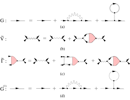
FIG. 2.: Feynman diagrams of the time-dependent Hartree-Fock approximation. Solid lines are single particle Green’s function and wavy lines are Coulomb interaction. Single(double) lines are bare(dressed) Green’s function and/or interaction: (a) the self-consistent Hartree-Fock approximation for the single electron Green’s function; (b) and (c) are respectively the Dyson’s equations for electron-electron interaction, single electron Green’s function and vertex function in the time-dependent Hartree-Fock approximation. The second term of (c) is the ladder series, while the third term is the bubble series (RPA diagram), which does not appear when calculating the vertex function for spin-flip excitations (since the interaction is spin-conserving) as mentioned in the text. (d) is the Green’s function in the first order Hartree-Fock approximation.

 

FIG. 3.: Energy level configuration for electron-hole pair excitations. Solid(dashed) lines are for spin down(up) levels with level index in the left hand side (the first orbital level index is set to be zero), and the upward arrow represents an electron-hole excitation (a magnetic exciton). (a) is for the two $2\times 2$ matrix representation of Eqs. (61) and (64): electron-hole pairs of numbers 1 and 2 are for $Y_{\sigma}$, and numbers 3 and 4 are for $Y_{\rho}$ respectively. (b) shows the configuration for one spin-flip excitation ($\delta\sigma=+1$) including next higher order energy excitations, which are beyond the TDHFA developed in the paper. (Note that in (b), the excitation from level $n$ to $n+2$ does not couple to pair number 1 due to parity symmetry in a parabolic well.)

 

FIG. 4.: Magnetoplasmon dispersions for $\nu=6$ and $B_{\|}$ (along $x$ direction) is 11 Tesla, calculated from Eqs. (66) and (68). (a) and (b) are for momentum along $x$ and $y$ directions respectively. Thick(thin) lines are for wavefunctions calculated from self-consistent Hartree-Fock and from first order Hartree-Fock approximations respectively.

 

FIG. 5.: Charge mode dispersion, $\omega_{\rho}(\vec{q}_{\perp})$, of magnetoplasmon excitations of the same system as used in Fig. 4 but for different filling factors, $\nu=2$, 4, 6 and 8, for comparison.

 

FIG. 6.: Same as Fig. 5, but for spin mode, $\omega_{\sigma_{+}}(\vec{q}_{\perp})$, dispersion.

 

FIG. 7.: Charge mode dispersion of magnetoplasmon excitation of the same system as used in Fig. 4 but with different confinement energy, $\omega_{0}$, at filling factor, $\nu=6$. Zero field well widths are about 260, 200, 175, and 155Å, corresponding to $\omega_{0}=7$, 11, 15, and 19 meV respectively. The parallel magnetic field is 11 Tesla for all results.

 

FIG. 8.: Same as Fig. 7, but for spin mode dispersion.

 

FIG. 9.: Charge mode magnetoplasmon dispersions for $\nu=1$, $B_{\perp}$=3 Tesla, and $\omega_{0}=3$ meV, calculated in the TDHFA. Solid, dotted, and dashed lines are for $B_{\|}=20$, 25, and 30 Tesla respectively, showing a charge mode softening in $y$ direction, perpendicular to the $B_{\|}$ direction. (a) and (b) are for wavevectors along $x$ and $y$ directions respectively.

 

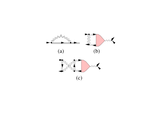
FIG. 10.: (a) The screened exchanged energy and (b) the screened ladder diagrams used in the screened TDHFA developed in Sec. IV (see Fig. 2). The interaction lines of the direct (Hartree) energy and the RPA diagrams are not screened to avoid double counting. (c) A diagram not included in the screened TDHFA but of the same order as a screened ladder diagram shown in (b). All notations are the same as those in Fig. 2.

 

FIG. 11.: Static dielectric function in momentum space for $\nu=6$ and $\omega_{0}=7$ meV. Solid and dashed lines represent $\epsilon(q_{x},q_{y}=0)$ and $\epsilon(q_{x}=0,q_{y})$ respectively. Thick and thin lines are for $B_{\|}=11$ and $8$ T.

 

FIG. 12.: Dispersions of magnetoplasmon excitations for $\nu=6$ in both charge ($\rho$) and spin ($\sigma_{+}$) modes including RPA screening (Eq. (108)) of the Coulomb interaction for $B_{\|}=11$ and 12 Tesla (dashed and solid lines respectively). Results of unscreened dispersion are also shown (dotted lines, the same as Fig. 4)) for comparison.

REFERENCES

• [1] For review, see for example, R.E. Prange and S.M. Girvin, The Quantum Hall Effect (Springer-Verlag, New York,1990); T. Chakraborty and P. Pieti$\ddot{\rm{a}}$inen, The Quantum Hall Effects — Fractional and Integral, 2nd ed. (Springer-Verlag Berlin Heidelberg, New York, 1995); S. Das Sarma and A. Pinczuk, Perspectives in Quantum Hall Effects (John Wiley & Sons, New York, 1997), and reference there in.
• [2] S. He, S. Das Sarma, and X.C. Xie, Phys. Rev. B 47, 4394 (1993); S. Das Sarma and E. Demler, Solid State Commun. 117, 141 (2001); T. Jungwirth and A.H. MacDonald, Phys. Rev. B 63, 035305 (2001).
• [3] S.M. Girvin and A.H. MacDonald, in Perspectives in Quantum Hall Effects of Ref. [1].
• [4] L. Zheng, R.J. Radtke, and S. Das Sarma, Phys. Rev. Lett. 78, 2453 (1997); S. Das Sarma, S. Sachdev, and L. Zhang, Phys. Rev. B 58, 4672 (1998); Phys. Rev. Lett. 79 917 (1997); E. Demler and S. Das Sarma, Phys. Rev. Lett. 82, 3895 (1999).
• [5] V. Pellegrini, A. Pinczuk, B.S. Dennis, A.S. Plaut, L.N. Pfeiffer, and K.W. West, Science 281 799 (1998); Phys. Rev. Lett. 78, 310 (1997).
• [6] A. Sawada, Z.F. Ezawa, H. Ohno, Y. Horikoshi, Y. Ohno, S. Kishimoto, F. Matsukura, M. Yasumoto, and A. Urayama, Phys. Rev. Lett. 80, 4534 (1998).
• [7] W. Pan, H.L. Stormer, D.C. Tsui, L.N. Pfeiffer, K.W. Baldwin, and K.W. West, Phys. Rev. B 64, 121305 (2001).
• [8] C.S. Sergio, G.M. Gusev, J.R. Leite, E.B. Olshanetskii, A.A. Bykov, N.T. Moshegov, A.K. Bakarov, A.I. Toropov, D.K. Maude, O. Estibals, and J.C. Portal, Phys. Rev. B 64, 115314 (2001)
• [9] Y.M. Suen, J. Jo, M.B. Santos, L.W. Engel, S.W. Hwang, and M. Shayegan, Phys. Rev. B 44, 5947 (1991).
• [10] C. Kallin and B. Halperin, Phys. Rev. B 30, 5655 (1984). Earlier work on 2D magnetoplasmon excitations can be found in Y.A. Bychkov, S.V. Lordanskii, and G.M.$\acute{{\rm E}}$liashberg, JETP Lett, 33, 143 (1981).
• [11] B.I. Halperin, Jpn. J. Appl. Phys. 26, Suppl. 26-3, 1913 (1987); M. Shayegan, T. Sajoto, M. Santos, and C. Silvestre, Appl. Phy. Lett. 53, 791 (1988).
• [12] L. Brey, N.F. Johnson, and B.I. Halperin, Phys. Rev. B 40, 10647 (1989).
• [13] Q.P. Li, K. Karrai, S.K. Yip, S. Das Sarma, and H.D. Drew, Phys. Rev. B 43, 5151 (1991); S.K. Yip, Phys. Rev. B, 40, 3882 (1989).
• [14] L. Brey, J. Dempsey, N.F. Johnson, and B.I. Halperin, Phys. Rev. B 42, 1240 (1990).
• [15] P.I. Tamborenea and S. Das Sarma, Phys. Rev. B 49, 16593 (1994).
• [16] As discussed in Sections II A and IV B, the in-plane magnetic field effectively enhances the confinement potential of a parabolic well. Therefore any small deviation of the bare confinement potential from a perfect parabolic one is relatively less important when a strong in-plane magnetic field is applied. Also if needed, nonparabolic effects can be included in our analysis simply by calculating the matrix element in the corresponding noninteracting basis (see Appendix A), which has to be carried out numerically for nonparabolic confinement potentials.
• [17] V. Celli and N.D. Mermin, Phys. Rev. 140, A839 (1965).
• [18] C.E. Hembree, B.A. Mason, J.T. Kwiatkowski, and J.E. Furneaux, Phys. Rev. B 50, 15197 (1994); M.P. Stopa and S. Das Sarma, Phys. Rev. B 40, 10048 (1989).
• [19] L. Brey and B.I. Halperin, Phys. Rev. B 40, 11634 (1989).
• [20] S. Das Sarma and P.I. Tamborenea, Phys. Rev. Lett 73, 1971 (1994); R.J. Radtke, P.I. Tamborenea, and S. Das Sarma, Phys. Rev. B 54, 13832 (1996).
• [21] L. Brey, Phys. Rev. B 44, 3772 (1991).
• [22] For a review of liquid crystal physics in quantum Hall systems, see M.M. Fogler, cond-mat/0111049 (unpublished).
• [23] M.P. Lilly, K.B. Cooper, J.P. Eisenstein, L.N. Pfeiffer, and K.W. West, Phys. Rev. Lett. 82, 394 (1999); R.R. Du, D.C. Tsui, H.L. Stormer, L.N. Pfeiffer, K.W. Baldwin, and K.W. West, Solid State Commun. 109, 389 (1999).
• [24] T. Jungwirth, A.H. MacDonald, L. Smrcka, and S.M. Girvin, Phys. Rev. B 60, 15574 (1999).
• [25] L. Brey and H. Fertig, Phys. Rev. B 62, 10268 (2000).
• [26] E. Demler, D.W. Wang, S. Das Sarma and B.I. Halperin, cond-mat/0110126; Solid state Commun. (in press).
• [27] A.L. Fetter and J.D. Walecka, Quantum Theory of Many-particle System (McGraw-Hill, New York, 1971).
• [28] C. Kittel, Quantum Theory of Solids (John Wiley & Sons, New York, 1987).
• [29] J. Dempsey and B. Halperin, Phys. Rev. B 45, 1719 (1992); ibid. 47, 4662 (1993); ibid. 47, 4674 (1993).
• [30] I.K. Marmorkos and S. Das Sarma, Phys. Rev. B 48, 1544 (1993).
• [31] T.D. Stanescu, I. Martin, and P. Phillips, Phys. Rev. Lett. 84, 1288 (2000).
• [32] T.M. Rice, Ann. Phys. 31, 100 (1965).
• [33] A. Pinczuk, J.P. Villadares, D. Heiman, A.C. Gossard, J.H. English, C.W. Tu, L. Pfeiffer, and K. West, Phys. Rev. Lett. 61, 2701 (1988); Surf. Sci. 229, 384 (1990).
• [34] D.W. Wang, E. Demler, S. Das Sarma, and B.I. Halperin, unpublished.
• [35] I.L. Aleiner and L.I. Glazman, Phys. Rev. B 52, 11296 (1995).
• [36] A. Lopatnikova, S.H. Simon, B.I. Halperin, X.-G. Wen, Phys. Rev. B 64, 155301 (2001).
• [37] There are dual purposes for our development of the screening theory in this work. The first is simply to develop an improved static theory of screening in the quantum Hall situation which transcends the simple theory of Ref. [35], and includes ladder diagrams in the polarizability function by going beyond the RPA. This is the primary motivation for our developing the screening theory including the ladder-exchange diagrams in the polarizability. We believe this to be a qualitative improvement on the ordinary Hartree-Fock screening, but it is difficult to precisely quantify the improvement. The second (and equally important) reason for our screening theory is to obtain the collective mode dispersion in an ”improved” approximation where screened static exchange diagrams have been included in calculation. The screened static exchange approximation developed by us in this work in the quantum Hall regime is similar to the widely used Hubbard approximation (J. Hubbard, J. Proc. R. Soc. London Ser. A 243, 336 (1957)) in the electron gas problem.
• [38] S.L. Sondhi, A. Karlhede, and S.A. Kivelson, and E.H. Rezayi, Phys. Rev. B 47, 16419 (1993).
• [39] U. Zeitler, H.W. Schumacher, A.G.M. Jansen, and R.J. Haug, Phys. Rev. Lett. 86, 866 (2001).
• [40] W. Kohn, Phys. Rev. 123, 1242 (1961).