Semiclassical theory of current correlations in chaotic dot-superconductor systems.

Abstract

We present a semiclassical theory of current correlations in multiterminal chaotic dot-superconductor junctions, valid in the absence of the proximity effect in the dot. For a dominating coupling of the dot to the normal terminals and a nonperfect dot-superconductor interface, positive cross correlations are found between currents in the normal terminals. This demonstrates that positive cross correlations can be described within a semiclassical approach. We show that the semiclassical approach is equivalent to a quantum mechanical Green’s function approach with suppressed proximity effect in the dot.

Over the last decade, there has been an increasing interest in current correlations in mesoscopic conductors. Buttikerrew Compared to the conductance, the current correlations contain additional information about the transport properties such as the effective charge or the statistics of the quasiparticles. Systems such as e.g. disordered conductors and chaotic quantum dots have been analyzed extensively, both with quantum mechanical approaches, using random matrix theoryBeenakker92 ; vanlangen97 or Green’s functions,Altshuler94 as well as with semiclassical approaches, based on the Boltzman-LangevinNagaev92 ; deJong96 ; Sukhorukov99 ; Blanter00 ; Blanter01 equation or voltage probe models.deJong96 ; vanlangen97 ; Blanter01

Recently, current correlations in normal-superconducting systems have been studied, theoretically Buttikerrew as well as experimentally.Jehl00 In these systems, the current into the superconductor is transported, at subgap energies, via Andreev reflection at the normal-superconducting interface. In the normal conductor, Andreev reflection induces a proxmity effect which modifies the transport properties at energies of the order of or below the Thouless energy.Lambert However, at energies well above the Thouless energy or in the presence of a weak magnetic field in the normal conductor, the proximity effect is suppressed.

Nagaev and one of the authorsNagaev01 presented a semiclassical Boltzman-Langevin approach, in the absence of the proximity effect, for current correlations in multiterminal diffusive normal-superconducting junctions, an extension of the corresponding approach for purely normal systems.Sukhorukov99 The interfaces between the normal conductor and the superconductor was assumed to be perfect. It was shown that the current cross correlations are manifestly negative, just as in normal mesoscopic conductors. Buttiker92 In contrast, it was shown very recently, taking the proximity effect into account, that in diffusive tunnel junctionsBoerlin02 and chaotic dot juctions,Samuelsson02 the ensemble averaged cross correlations can be positive.

Interestingly, as shown for the chaotic dot juction, Samuelsson02 in the limit of strong coupling of the dot to the normal reservoirs and a nonperfect normal-superconducting interface, positive cross correlations can survive even in the abscence of the proximity effect. This suggests that positive current correlations could be obtained within a semiclassical approach, under the assumption of a suppressed proximity effect, if nonperfect normal-superconductor interfaces are assumed.

In this paper we present such a semiclassical theory for multiterminal chaotic dot-superconductor junctions with arbitrary transparencies of the contacts between the dot and the normal and superconducting reservoirs. It confirmes and extends the result of Ref. [Samuelsson02, ], providing conditions on the contact widths and transparencies for obtaining positive correlations. We show that the result is in agreement with the circuit theory of Refs. [Nazarov, ; Boerlin02, ] with suppressed proximity effect in the dot. This provides a simple, semiclassical explanation for the positive cross correlations.

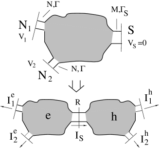
Figure 1: Upper figure: A schematic picture of the junction. Lower figure: Mapping onto an electron-hole junction (see text). The arrows show the direction of particle current flows.

A schematic picture of the system is shown in Fig. 1. We consider a chaotic quantum dot (see Ref. [Beenakker97, ] for definition) connected to two normal ($N_{1}$ and $N_{2}$) and one superconducting reservoir ($S$) via quantum point contacts. The contacts to the normal and superconducting reservoirs have mode independent transparencies $\Gamma$ and $\Gamma_{S}$ respectively and support $N$ and $M$ transverse modes.

The conductances of the point contacts are much larger than the conductance quanta $2e^{2}/h$, i.e. $N\Gamma,M\Gamma_{S}\gg 1$, so Coulomb blockade effects in the dot can be neglected. The two normal reservoirs are held at the potentials $V_{1}$ and $V_{2}$ and the potential of the superconducting reservoir is zero. Inelastic scattering in the dot is neglected. Throughout the paper, we consider the case where $V_{1},V_{2},kT\ll\Delta$, where $\Delta$ is the superconducting gap. In this case, the probability for Andreev reflection at the normal-superconductor interface, $R=\Gamma_{S}^{2}/(2-\Gamma_{S})^{2}$, is independent of energy and there is no single particle transport into the superconductor. commentvolt

The semiclassical approach for current correlations in normal chaotic dot systems has been developed within a voltage probe approach vanlangen97 ; Blanter01 or equivalently, a minimal correlation approach. Blanter00 ; Blanter01 ; Oberholzer01 Here we extend it to a chaotic dot-superconductor system, shown in Fig. 1, by first considering the particle current correlations in the dot-superconductor system. To visualize the particle current flow, it is helpful to view the chaotic dot-superconductor system as one “electron dot” and one “hole dot”, coupled via Andreev reflection (see Fig. 1). Due to the abscence of the proximity effect, the electron and hole dots can be treated as two coupled, independent dots, and one can calculate the particle current correlations in the same way as in a purely normal system (Andreev reflection conserves particle currents). From the particle current correlations, we then obtain the experimentally relevant charge current correlations.

We study the zero-frequency correlator

$$P_{jk}=2\int dt~{}\langle\Delta I_{j}(t)\Delta I_{k}(0)\rangle$$ (1)

between charge currents flowing in the contacts $j=1,2$ to the normal reservoirs, where $\Delta I_{j}(t)=I_{j}(t)-\bar{I}_{j}$ is the current fluctuations in lead $j$ ($\bar{I}_{j}$ is the time averaged current). The charge current $I_{j}(t)$ is the difference of the electron (e) and hole (h) particle currents,

$$I_{j}(t)=I^{e}_{j}(t)-I^{h}_{j}(t),~{}~{}I_{j}^{\alpha}(t)=\frac{e}{h}\int dE~{}i_{j}^{\alpha}(E,t),$$ (2)

where the particle currents densities $i_{j}^{\alpha}(E,t)=\bar{i}_{j}^{\alpha}(E)+\Delta i_{j}^{\alpha}(E,t)$. The electron current density flowing into the superconductor is $i_{S}^{e}(E,t)\equiv i_{S}(E,t)=-i_{S}^{h}(E,t)$.

First, the time average current is studied. Using the requirement of current conservation at each energy [due to the abscence of inelastic scattering], the time averaged electron and hole distribution functions $\bar{f}_{e}$ and $\bar{f}_{h}$ can be determined. We have for each dot separately [suppressing the energy notation]

$$\bar{i}_{1}^{e}+\bar{i}_{2}^{e}+\bar{i}_{S} = 0,~{}\bar{i}_{1}^{h}+\bar{i}_{2}^{h}-\bar{i}_{S}=0.$$ (3)

The currents $\bar{i}_{j}^{\alpha}$ and $\bar{i}_{S}$ flowing through the point contacts are given by

$$\bar{i}_{j}^{\alpha} = N\Gamma\left[\bar{f}^{\alpha}-f^{\alpha}_{j}\right],~{}\bar{i}_{S}=MR[\bar{f}^{e}-\bar{f}^{h}],$$ (4)

where $f_{j}^{\alpha}=[1+\mbox{exp}([E\pm eV_{j}]/kT)]^{-1}$ is the distribution function of quasiparticle type $\alpha$ of the normal reservoir $j$, with $-(+)$ for electrons (holes). Combining Eq. (3) with Eq. (4), we obtain

$$\bar{f}^{e}=\frac{MR(f_{1}^{h}+f_{2}^{h})+(2N\Gamma+MR)(f_{1}^{e}+f_{2}^{e})}{4(N\Gamma+MR)},$$ (5)

and similarily $\bar{f}^{h}=\bar{f}^{e\rightarrow h}$, where we note that $\bar{f}^{h}(E)=1-\bar{f}^{e}(-E)$, as demanded by electron-hole symmetry. We can then calculate the time averaged currents from Eq. (4) and (2). This is however not further discussed here.

We now turn to the fluctuating part of the current. The point contacts emit fluctuations $\delta i_{j}^{\alpha}$ and $\delta i_{S}$, directly into the reservoir as well as into the dot. As a consequence the electron and hole distribution functions aquires a fluctuating part,vanlangen97 ; Blanter00 $f^{\alpha}(t)=\bar{f}^{\alpha}+\delta f^{\alpha}(t)$. The total fluctuating current in each contact is given by (suppressing the time notation)

$$\Delta i_{j}^{\alpha}=\delta i_{j}^{\alpha}+N\Gamma\delta f^{\alpha},~{}\Delta i_{S}=\delta i_{S}+MR(\delta f^{e}-\delta f^{h}).$$ (6)

The fluctuating parts of the distribution functions, $\delta f^{e}$ and $\delta f^{h}$, are determined from the demand that the fluctuating current, in the zero frequency limit considered, is conserved in each dot,

$$\Delta i_{1}^{e}+\Delta i_{2}^{e}+\Delta i_{S}=0,~{}\Delta i_{1}^{h}+\Delta i_{2}^{h}-\Delta i_{S}=0.$$ (7)

Solving these two equations gives $\delta f^{e}$ and $\delta f^{h}$, which can be substituted back into Eqs. (6) to give the fluctuating currents in the leads $\Delta i_{j}^{\alpha}$ in terms of the fluctuating currents emitted by the point contacts $\delta i_{j}^{\alpha}$ and $\delta i_{S}$. The charge current fluctuations in contact $1$ and $2$ is then found by subtracting the electron and the hole currents, i.e. $\Delta i_{j}=\Delta i_{j}^{e}-\Delta i_{j}^{h}$, giving

$$\Delta i_{1}=\frac{(N\Gamma+2MR)[\delta i_{1}^{e}-\delta i_{2}^{h}]+N\Gamma(\delta i_{1}^{h}-\delta i_{2}^{e}+2\delta i_{S})}{2(N\Gamma+MR)}$$

(8)

and $\Delta i_{2}=\Delta i_{1\rightarrow 2}$. For the second moment, the point contacts can be considered cumulantcom as independent emitters of fluctuations, i.e. (here including $\delta i_{S}$)

$$\langle\delta i_{j}^{\alpha}(E,t)\delta i_{k}^{\beta}(E^{\prime},t^{\prime})\rangle=\frac{h}{e}\delta_{jk}\delta_{\alpha\beta}\delta(E-E^{\prime})\delta(t-t^{\prime})S_{j}^{\alpha}$$ (9)

where the fluctuation power $S_{j}^{\alpha}(E)$ is determined by the transparency of contact $j$ and the time averaged distribution functions on each side of the contact, Buttiker92 as

$$S_{j}^{\alpha}(E) = eN\Gamma[f^{\alpha}_{j}(1-f^{\alpha}_{j})+\bar{f}^{\alpha}(1-\bar{f}^{\alpha})$$

$$+ (1-\Gamma)(\bar{f}^{\alpha}-f^{\alpha}_{j})^{2}],$$

$$S_{S}(E) = eMR[\bar{f}^{e}(1-\bar{f}^{e})+\bar{f}^{h}(1-\bar{f}^{h})$$ (10)

$$+ (1-R)(\bar{f}^{e}-\bar{f}^{h})^{2}].$$

Eqs. (1) to (10) form a complete set of equations to calculate the current correlations.

As an example, which also allows a comparison to Ref. [Samuelsson02, ], we study the current cross correlations $P_{12}$ for $V_{1}=V_{2}=V$ and $kT=0$. In this limit only the energy interval $0<E<eV$ is of interest, where $f^{e}_{1}=f^{e}_{2}=1$ and $f^{h}_{1}=f^{h}_{2}=0$. Correlating the current density fluctuations $\Delta i_{1}$ and $\Delta i_{2}$ in Eq. (8) and using the expressions for the power spectra in Eq. (10), with the distribution functions $\bar{f}^{e}$ and $\bar{f}^{h}$ taken from Eq. (5), we obtain from Eq. (2) and (1) for the the cross-correlator

$$P_{12} = V\frac{e^{3}}{h}\frac{N^{2}M\Gamma^{2}R}{(N\Gamma+MR)^{4}}[2\Gamma^{2}N^{2}(1-2R)$$ (11)

$$- MR(N\Gamma[2-\Gamma]+2MR[1-\Gamma])].$$

In the limit without barriers, $\Gamma=1$ and $R=1$, as well as in the limit $\Gamma=1$ and $N\gg M$, this expression coincides with the random matrix theory result available in Ref. [Samuelsson02, ]. From Eq. (11), we can make the following observations. In the limit of dominating coupling to the superconductor, $MR\gg N\Gamma$, the cross correlations are manifestly negative (see Fig. 2). The positive correlations predicted in this limit in Refs. [Boerlin02, ; Samuelsson02, ] are thus due to the proximity effect.

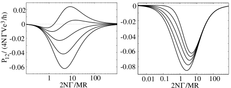
Figure 2: The cross correlation $P_{12}$ as a function of the ratio of the conductances of the point contacts to the normal and superconducting reservoirs, $2N\Gamma/MR$, for different barrier transparencies. Left: $\Gamma=1$ and from bottom to top $R=1,0.8,0.6,0.4$ and $0.2$. Right: $R=1$ and from top to bottom, $\Gamma=1,0.8,0.6,0.4$ and $0.2$.

In the opposite limit, dominating coupling to the normal reservoirs $N\Gamma\gg MR$, the correlations are $P_{12}\propto R(1-2R)$, positive for $R<1/2$.

In the general case, with different transparencies or widths of the two contacts to the normal reservoirs, an asymmetric bias $V_{1}\neq V_{2}$ or finite temperatures, a detailed study shows that the conditions $R<1/2$ and a dominating coupling of the dot to the normal reservoirs are still necessary, but not always sufficient, for positive cross correlations. The junction parameters of the example studied above are the most favorable for obtaining positive correlations.

We now show that the result in Eq. (11) can be obtained by an ensemble averaged, quantum mechanical Green’s function approach, when supressing the proximity effect with a weak magnetic field in the dot. We apply the circuit theory of Refs. [Nazarov, ; Boerlin02, ], which is formulated to treat the full counting statistics of the charge transfer. The formulation of the problem is similar to Ref. [Boerlin02, ], so we keep the description short. However, we treat arbitrary contact transparencies and finite magnetic field in the dot.

A picture of the circuit is shown in Fig. 3. It consists of four “nodes”, the normal and superconducting reservoirs and the dot itself, connected by “resistances”, the point contacts. Each node is represented by a $4\times 4$ matrix Greens functions (see Fig. 3).

Figure 3: Left: The circuit theory representation of the junction with the Greens functions of each node and the counting fields shown. Right: The particle counting model. (see text)

The Greens functions of the reservoir nodes are known, given by $\check{G}_{Nj}=\mbox{exp}(i\chi_{j}\check{\tau}_{K}/2)\check{G}_{N}\mbox{exp}(-i\chi_{j}\check{\tau}_{K}/2)$ and $\check{G}_{S}=\mbox{exp}(i\chi\check{\tau}_{K}/2)\bar{1}\hat{\sigma}_{x}\mbox{exp}(-i\chi\check{\tau}_{K}/2)$, where $\check{G}_{N}=\bar{\tau}_{z}\hat{\sigma}_{z}+(\bar{\tau}_{x}+i\bar{\tau}_{y})\hat{1}$ and $\check{\tau}_{K}=\bar{\tau}_{x}\hat{\sigma}_{z}$. Here $\bar{\tau}(\hat{\sigma})$ are Pauli matrices in Keldysh (Nambu) space and $\chi_{1},\chi_{2}$ and $\chi$ are counting fields, “counting” the number of electrons entering and leaving the reservoirs. The unknown Green’s function $\check{G}(\chi_{1},\chi_{2},\chi)$ of the dot, normalized as $\check{G}^{2}=1$, is determined from a matrix version of the Kirchoffs rule,

$$\check{I}_{N1}+\check{I}_{N2}+\check{I}_{S}+\check{I}_{\Phi}=0$$ (12)

where the matrix currents $\check{I}_{N1},\check{I}_{N2}$ and $\check{I}_{S}$ are given by

$$\check{I}_{N1(2)} = N\Gamma[\check{G}_{N1(2)},\check{G}](4+\Gamma[\{\check{G}_{N1(2)},\check{G}\}-2])^{-1}$$

$$\check{I}_{S} = M\Gamma_{S}[\check{G}_{S},\check{G}](4+\Gamma_{S}[\{\check{G}_{S},\check{G}\}-2])^{-1},$$ (13)

where $[A,B](\{A,B\})$ is the (anti)commutator. The last current term, dominated by the presence of a magnetic field in the dot, is Volkov $I_{\Phi}=\gamma(h\Phi/e)^{2}[\check{\tau}_{0}\check{G}\check{\tau}_{0},\check{G}]$, where $\Phi$ is the magnetic flux in the dot, $\check{\tau}_{0}=\bar{1}\hat{\sigma}_{z}$ and $\gamma$ is a constant of order of $2N\Gamma,M\Gamma_{S}$, i.e. much larger than one. We are interested in the case with suppressed proximity effect, which can be achieved by applying a magnetic field corresponding to a flux $\Phi$ larger than a flux quantum. This implies that the $I_{\Phi}$ term in Eq. (12) is much larger than the other terms, and consequently that $[\check{\tau}_{0}\check{G}\check{\tau}_{0},\check{G}]=0$ to leading order in $1/\Phi^{2}$. The cross correlator $P_{12}$ is

$$P_{12}=Ve^{3}/h\mbox{tr}\left.\left[\check{\tau}_{K}\partial\check{I}_{N1}/\partial\chi_{2}\right]\right|_{\chi_{1}=\chi_{2}=\chi=0}.$$ (14)

It is not possible to find an explicit expression for $\check{G}(\chi_{1},\chi_{2},\chi)$ from Eq. (12) and the additional conditions $\check{G}^{2}=1$ and $[\check{\tau}_{0}\check{G}\check{\tau}_{0},\check{G}]=0$. However, to evaluate the correlator $P_{12}$, only $\partial\check{I}_{N1}/\partial\chi_{2}$ is needed, and consequently only the Green’s functions expanded to first order in $\chi_{2}$. We get $\check{G}=\check{G}^{(0)}+i(\chi_{2}/2)\check{G}^{(1)}$, where $\check{G}^{(n)}=\partial^{n}\check{G}/\partial\chi_{2}^{n}|_{\chi_{1}=\chi_{2}=\chi=0}$, and similar for the others. From Eq. (12), expanded to first order in $\chi_{2}$ as well, we then arrive at equations for $\check{G}^{(0)}$ and $\check{G}^{(1)}$.

The physically relevant result for $\check{G}^{(0)}$ is $\bar{\tau}_{z}\hat{\sigma}_{z}+h(\bar{\tau}_{x}+i\bar{\tau}_{y})\hat{1}$, where $h=N\Gamma/(N\Gamma+MR)$. Knowing $\check{G}^{(0)}$, and using that from $\check{G}^{2}=1$ we obtain $\{\check{G}^{(0)},\check{G}^{(1)}\}=0$, we then get $\check{G}^{(1)}=-h^{2}\bar{\tau}_{z}\hat{\sigma}_{z}+\tilde{h}(\bar{\tau}_{x}+i\bar{\tau}_{y})\hat{1}+h(\bar{\tau}_{x}-i\bar{\tau}_{y})\hat{1}$, where $\tilde{h}=-h[(1-2h+2h^{2})+\Gamma(h-1)^{3}+2h^{3}MR(2R-1)/(N\Gamma)]$. Inserting the expressions for $\check{G}^{(0)}$ and $\check{G}^{(1)}$ into $\partial I_{N1}/\partial\chi_{2}$, we find $P_{12}$ from Eq. (14). This gives exactly the semiclassical result in Eq. (11).

Finally, it was pointed out that in the limit of dominating coupling to the normal reservoirs, $N\Gamma\gg MR$, the simple expression for the cross correlations $P_{12}\propto R(1-2R)$ could be explained by particle counting arguments. Samuelsson02 We now show that the full probability distribution of transmitted charges in this limit can be derived from the circuit theory. The total cumulant generating function $F(\chi_{1},\chi_{2},\chi)$ is the sum of the functions for each point contact, $F=F_{N1}+F_{N2}+F_{S}$, where

$$F_{S}=eVM\Gamma_{S}~{}\mbox{tr}~{}\mbox{ln}[4+\Gamma_{S}(\{\check{G},\check{G}_{S}\}-2)],$$

$$F_{N1(2)}=eVN\Gamma~{}\mbox{tr}~{}\mbox{ln}[4+\Gamma(\{\check{G},\check{G}_{N1(2)}\}-2)].$$ (15)

We expand the Green’s function of the dot, $\check{G}$, to first order in $MR/N\Gamma$, (but no expansion in the counting fields). To zeroth order in $MR/N\Gamma$, the superconducting reservoir is disconnected, and we get directly $\check{G}^{(0)}=(\check{G}_{N1}+\check{G}_{N2})/2$. Since normalization implies $\{\check{G}^{(0)},\check{G}^{(1)}\}=0$, we note that the contribution to $F$ from the point contacts connected to the normal reservoirs, $F_{N1}+F_{N2}\propto\{\check{G}^{(0)},\check{G}^{(1)}\}$ disappears to first order in $N\Gamma\gg MR$. The total $F(\chi_{1},\chi_{2},\chi)$ is then obtained by inserting $\check{G}=\check{G}^{(0)}$ into Eq. (15), giving (for $V<0$)

$$F=eVM~{}\mbox{ln}\left[1-R+\frac{R}{4}\left(e^{i(\chi_{1}-\chi)}+e^{i(\chi_{2}-\chi)}\right)^{2}\right].$$ (16)

In the limit $R\ll 1$, $F$ has the same form as in Ref. [Boerlin02, ]. The corresponding probability distribution $P(Q,q_{1},q_{2})$ of Eq. (16), that $q_{1}(q_{2})$ particles have left the dot through contach 1(2) when $Q$ pairs have attempted to enter the dot, is (for even $q_{1}+q_{2}$) given by

$$P(Q,q_{1},q_{2})=\frac{Q!(q_{1}+q_{2})!}{q_{1}!q_{2}!(Q-[q_{1}+q_{2}]/2)!([q_{1}+q_{2}]/2)!}$$

$$\times\left(\frac{R}{4}\right)^{(q_{1}+q_{2})/2}(1-R)^{Q-(q_{1}+q_{2})/2}.$$ (17)

This is just the distribution function one gets from the model of Ref. Samuelsson02, . A filled stream of pairs are incoming from the superconductor. Each pair has a probability $R$ to enter the dot and then each particle in the pair has an independent probability $1/2$ to exit through one of the contacts $1$ or $2$ (see Fig. 3).

The processes where both particles exit through the same contact contributes $\propto-R^{2}$ to the cross correlations, while the processes where the pair breaks and one particle exits throgh each contact contributes $\propto R(1-R)$. Thus, for $R<1/2$, the pair breaking noise dominates over the pair partition noise and the cross correlations are positive. We emphasize that it is the fact that the superconductor emits particles in pairs that makes positive correlations possible, in a corresponding normal systems the electrons tries to enter the dot one by one and the cross correlations are manifestly negative.

In conclusion, we have presented a semiclassical theory of current-current correlations in multiterminal chaotic dot-superconducting junctions. It is found that the current cross correlations are positive for finite backscattering in the dot-superconducting contact and dominating coupling of the dot to the normal reservoirs. We have also shown that this approach is equivalent to an ensemble averaged Greens function approach with a suppressed proximity effect

We acknowledge discussions with W. Belzig, Y. Nazarov, H. Schomerus and E. Sukhorukhov. This work was supported by the Swiss National Science Foundation and the program for Materials with Novel Electronic Properties.

References

- (1) For a review, see Ya. M. Blanter and M. Büttiker, Phys. Rep. 336 1 (2000).
- (2) C.W.J. Beenakker and M. Büttiker, Phys. Rev. B 46 1889 (1992); R.A. Jalabert, J.-L Pichard and C.W.J. Beenakker, Europhys. Lett. 27 255 (1994).
- (3) S.A. van Langen and M. Büttiker, Phys. Rev. B. 56, R1680 (1997).
- (4) B.L. Altshuler, L.S. Levitov, and A. Yu. Yakovets, Pis’ma Zh. Eksp. Teor. Fiz. 59 821 (1994) [JETP Lett. 59, 857 (1994)]; Ya. M. Blanter and M. Büttiker, Phys. Rev. B 56, 2127 (1997).
- (5) K.E. Nagaev, Phys. Lett. A 169, 103 (1992).
- (6) E. V. Sukhorukov and D. Loss, Phys. Rev. B 59, 13054 (1999).
- (7) Ya. M. Blanter and E.V. Sukhorukov, Phys. Rev. Lett. 84, 1280 (2000).
- (8) Ya. M. Blanter, H. Schomerus and C.W.J. Beenakker, Physica E 11, 1 (2001).
- (9) M.J.M. de Jong and C.W.J. Beenakker, Physica A 230, 219 (1996).
- (10) X. Jehl et al., Nature (London) 405 50 (2000), A.A. Kozhevnikov, R.J. Shoelkopf, and D.E. Prober, Phys. Rev. Lett. 84 3398 (2000).
- (11) For a review, see C.J. Lambert and R. Raimondi, J. Phys. Condens. Matter 10, 901 (1998).
- (12) K. Nagaev and M. Büttiker, Phys. Rev. B 63 081301, (2001).
- (13) M. Büttiker, Phys. Rev. B 46, 12485 (1992).
- (14) J. Börlin, W. Belzig, and C. Bruder, Phys. Rev. Lett. 88, 197001 (2002).
- (15) P. Samuelsson and M. Büttiker, Phys. Rev. Lett. 89, 046601 (2002).
- (16) W. Belzig and Yu. V. Nazarov, Phys. Rev. Lett. 87, 197006 (2001); 87 067006 (2001).
- (17) C.W.J. Beenakker, Rev. Mod. Phys. 69, 731 (1997).
- (18) S. Oberholzer et al., condmat/0105403.
- (19) The approach can be extended to arbitrary voltages and temperatures, by taking into account the energy dependence of the Andreev refelction probability as well as single particle transport into the superconductors at (the latter done via an additional contact).
- (20) The fact that or are fluctuating themselves only affects higher moments of the current correlations, see K.E. Nagaev et al, (in preparation).
- (21) A.F. Volkov and A.V. Zaitsev, Phys. Rev. B 53 9267, (1996); W. Belzig, C. Bruder and G. Schön, ibid 54 9443, (1996).