Instability of the rhodium magnetic moment as origin of the metamagnetic phase transition in $\alpha$-FeRh

Abstract

Based on ab initio total energy calculations we show that two magnetic states of rhodium atoms together with competing ferromagnetic and antiferromagnetic exchange interactions are responsible for a temperature induced metamagnetic phase transition, which experimentally is observed for stoichiometric $\alpha$-FeRh. Taking into account the results of previous and newly performed first-principles calculations we present a spin-based model, which allows to reproduce this first-order metamagnetic transition by means of Monte Carlo simulations. Further inclusion of spacial variation of exchange parameters leads to a realistic description of the experimental magneto-volume effects in $\alpha$-FeRh.

I Introduction

In 1938 FallotFallot (1938); Fallot and Horcart (1939) discovered that ordered bcc Fe₅₀Rh₅₀ undergoes a first order metamagnetic transition from an antiferromagnetic (AF) ground state to a ferromagnetic (FM) phase with increasing temperature. This transition occurs at $T_{\rm m}\approx 320\,{\rm K}$ and is accompanied by a volume increase of about $1\,\%$.Kouvel (1966); Zakharov et al. (1964) The Curie temperature $T_{\rm C}$ of the FM phase is of the order of $670\,{\rm K}$.Zakharov et al. (1964); Kouvel and Hartelius (1962) In contradiction to the first hypothesis of Fallot and Horcart,Fallot and Horcart (1939) X-ray diffraction measurements showed that the transition is isostructural.de Bergevin and Muldawer (1961) From Mössbauer and neutron diffraction measurements one knows that the FM phase has collinear magnetic moments of $3.2\,\mu_{\rm B}$ per Fe atom and $0.9\,\mu_{\rm B}$ per Rh atom.Shirane et al. (1963) At low temperatures an AF-II spin structure is found with Fe moments of $3.3\,\mu_{\rm B}$ and with vanishing Rh moments (see Figure 1).Shirane et al. (1964); Kunitomi et al. (1971) Application of hydrostatic pressure suppresses the FM phase, i. e. for a critical pressure of $60\,{\rm kbar}$ the system immediately transforms from the AF to the paramagnetic (PM) phase.

An early explanation for this behavior was based on the phenomenological exchange inversion modelKittel (1960) by Kittel (which originally was designed to explain metamagnetic transitions in other materials like Cr-modified Mn₂Sb with a layered magnetic structure). In this model the exchange parameter varies linearly with the lattice constant and changes sign for a critical value $a_{\rm c}$. However, experimental findings like the rather large entropy changeKouvel (1966); Zakharov et al. (1964); Annaorazov et al. (1996); Lommel (1969); McKinnon et al. (1970) at $T_{\rm m}$, which is of the order of $\Delta S(T_{\rm m})\approx 12.5-19.7\,{\rm J\,kg^{-1}K^{-1}}$, as well as elastic properties could not correctly be described.McKinnon et al. (1970) Tu et al.Tu et al. (1969) used a different approach by considering the large difference of the low-temperature specific heat constants, $\gamma$, of the AF and the FM phases: Measurements suggest that $\gamma_{\rm FM}\approx 59-62.5\,{\rm mJ\,kg^{-1}K^{-2}}$ is about four to six times larger than $\gamma_{\rm AF}\approx 10.5-16\,{\rm mJ\,kg^{-1}K^{-2}}$.Tu et al. (1969); Ivarsson et al. (1971) Based on these observations, Tu et al. explained the transition by a change in entropy of the band electrons between the AF and the FM phases. An estimation of the free energy shows that these contributions have the right order of magnitude to explain the AF–FM transition, if one assumes that the electronic densities of states at the Fermi level do not vary considerably from low temperatures up to the transition. However, since the FM phase cannot be stabilized at low temperatures for stoichiometric FeRh, $\gamma_{\rm FM}$ has been measured in slightly more iron-rich alloys. With respect to the strong sensitivity of the magnetic phase diagram to small departures from stoichiometry,Vinokurova et al. (1988) one may doubt that the low temperature specific heat can be considered to be independent of concentration.Ponomarev (1972); Moruzzi and Marcus (1992a) A further drawback considering the explanation of Tu et al. arises from the fact that adding $5\,\%$ Iridium boosts $\gamma_{\rm AF}$ by almost an order of magnitude to a value of $\gamma_{\rm AF}=101\,{\rm mJ\,kg^{-1}K^{-2}}$:Ivarsson et al. (1971); Fogarassy et al. (1972) The compound Fe_49.5Rh_45.5Ir₅ also undergoes a metamagnetic transition with $T_{\rm m}$ shifted to higher temperatures.Kouvel (1966) Since the relation between $\gamma_{\rm AF}$ and $\gamma_{\rm FM}$ is reversed in this material, the previously sketched explanation cannot be applied to this case.

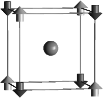
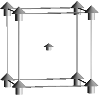
Figure 1: Left: Type II antiferromagnetic ground state structure with a nonmagnetic Rh atom at the center and Fe atoms with moments of $3.3\,\mu_{\rm B}$ at the corner site. Right: Ferromagnetic structure with Fe moments of $3.2\,\mu_{\rm B}$ at the corners and Rh moment of $0.9\,\mu_{\rm B}$ at the center site.

In 1992 Moruzzi and Marcus performed ab initio calculations using spin polarized density functional theory (DFT) in the framework of the local density approximation (LDA) and the augmented spherical wave (ASW) formalism.Moruzzi and Marcus (1992a); Moruzzi and Marcus (1992b); Moruzzi and Marcus (1993) They calculated the total energy of FeRh as a function of volume for different magnetic structures. They found that the AF-II spin structure is the ground state, whereas the FM structure is another stable solution with higher energy and a larger volume. For the moments they obtained $\mu_{\rm Fe}=2.98\,\mu_{\rm B}$, $\mu_{\rm Rh}=1.02\,\mu_{\rm B}$ (AF phase) and $\mu_{\rm Fe}=3.15\,\mu_{\rm B}$ (FM phase), in agreement with experimental results.

In this work, we present further ab initio total energy calculations of stoichiometric $\alpha$-FeRh using the ASW formalism and the generalized gradient approximation (GGA).Perdew et al. (1992) The corresponding code also allows to evaluate noncollinear alignment of spins (see Ref. Uhl et al., 1994 and references therein). For many cases LDA gives a reasonable description of the ground state properties of solids. However, in some cases it predicts the wrong ground state as e. g. for ironStixrude et al. (1994). For Fe, the hcp structure is found to be $10\,$mRy lower in energy than the bcc phase. Because FeRh has also a bcc ground state lattice structure (unlike pure Rh), it is necessary to go beyond LDA by using GGA. We have considered different possible magnetic ground state structures presented in section II. Based then on the specific energetic order of resulting energy versus volume curves, we discuss a new mechanism for the temperature driven metamagnetic transition in FeRh. In contrast to prior explanations, our model does not rely on ground state properties or low temperature data alone. Instead, we propose that thermal excitations at finite temperatures are the driving force for the transition. This is demonstrated in section III on the basis of Monte Carlo simulations of an Ising-type spin model, showing that a competition between AF Fe-Fe exchange-interactions and a nonmagnetic Rh state on the one hand and FM Fe-Rh interactions on the other is sufficient to explain the metamagnetic transition of FeRh. Inclusion of spatial degrees of freedom (section IV) by adding pair potentials and assuming a linear variation of the exchange parameter with the lattice parameter proves that this model explanation is in accordance with the ab initio data and leads furthermore to a nearly quantitative description of experimental details.

II Ab initio total energy calculations

$V_{\rm 0}$		$\Delta E$	$m_{\rm Fe}$		$B$		$N(E_{\rm F})$
	a.u./atom		mRy	$\mu_{\rm B}$		GPa		states/Ry
	AF	FM		AF	FM	AF	FM	AF	FM
Ref. Moruzzi and Marcus,1992a	90.2	91.8	1.9	2.98	3.15	214	202	37	32
Ref. Szajek and Morkowski,1994	91.9	92.9	2.2	3.13	3.20	227	244	13	32
This work	91.4	93.0	2.5	3.18	3.23	197	193	13	29

Table 1: Comparison of ab initio results.Here, $V_{\rm 0}$ is the equilibrium volume of AF and FM phases, $\Delta E=E_{\rm FM}-E_{\rm AF}$ is the energy difference per atom, $m_{\rm Fe}$ is the Fe magnetic moment, $B$ is the bulk modulus, and $N(E_{\rm F})$ the density of states per formula unit at the Fermi level. The moment on the Rh sites is $1.0\,\mu_{\rm B}$ in the FM phase and zero in the AF phase in all calculations.

We have performed ab initio calculations by using the ASW-method Williams et al. (1979) and GGA. Relativistic effects are included in the scalar relativistic approximation. The basis wave functions of Fe and Rh atoms include spd and f states which are sufficient to obtain the correct magnetic behavior of $\gamma$-iron. We assume that the AF like spin structure can best be described by a spin-spiral (Ref. Uhl et al., 1994) with wave vector $(0.5,0.5,0.5)$ in units of $2\pi/a$. As first step, we optimized the volume of the AF-II state with equal ASA-radii for both types of atoms. For the resulting equilibrium volume, the total energy is then minimized with respect to the ratio of the ASA-spheres leading to $r_{\rm Rh}/r_{\rm Fe}=1.15$. In order to investigate the influence of the Rh moment in the FM phase we have also used the fixed spin moment method Uhl et al. (1994) to restrict $m_{\rm Rh}$ to zero.

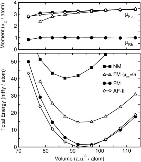
Figure 2: Total energy and magnetic moment versus atomic volume as obtained by ab initio calculations (present work).

Table 1 contains the calculated equilibrium properties for AF-II and FM phases which are in fair agreement with previous calculations. Compared to previous non-relativistic ASW LDA calculations (Moruzzi et al.Moruzzi and Marcus (1992a)), we obtain equilibrium volumes which are about 1-2$\,\%$ larger, being typical for GGA. In contrast to the cases of pure ironHerper et al. (1999) and $\mathrm{FeNi}$ Invar alloysBarbiellini et al. (1991), the magnetic energy differences are only slightly influenced by the gradient corrections. Also, no evidence was found that a noncollinear structure could be lower in energy than the previously found collinear AF and FM spin arrangements. With respect to the density of states at the Fermi level our results compare better with results of Szajek et al.Szajek and Morkowski (1994) than with results of Ref. Moruzzi and Marcus, 1992a. Since the latter results were obtained by using LDA ASW (with a spd basis), we conclude that the density of states at the Fermi level is very sensitive to computational details. The values obtained for the bulk moduli, $B_{\rm AF}$ and $B_{\rm FM}$, are lower compared to those of Ref. Moruzzi and Marcus, 1992a (where $B_{\rm AF}>B_{\rm FM}$ was obtained in contrast to $B_{\rm FM}>B_{\rm AF}$ in Ref. Szajek and Morkowski, 1994).

The calculated total energy curves are shown in Fig. 2. The large energetic difference between the usual FM phase and the hypothetic FM phase with zero rhodium moment implies that a finite Rh moment plays an important role for the stability of the FM phase. It seems unlikely that a magnetic field at the Rh sites induced by the surrounding iron atoms is responsible for the appearance of a Rh moment in the FM phase, as was proposed in previous discussions. However, a strong ferromagnetic exchange interaction between the Rh and the iron atoms that overrides an antiferromagnetic exchange between next nearest neighbor iron sites, would explain how the existence of a Rh moment can help to stabilize the FM phase. We have evidence as shown in the following sections, that a competition between a low lying nonmagnetic Rh state and another one with higher energy and finite moment (which can benefit from exchange with ferromagnetic iron neighbors) is the main reason for the metamagnetic transition.

III A spin-analogous model

In order to confirm our hypothesis we have constructed a model being suitable for an examination of the metamagnetic transition at finite temperatures. The simplest way to do this is by means of Monte Carlo simulations with a localized spin model. To keep the model tractable, we neglect spin wave excitations and restrict ourselves to Ising spins. This is justified because the transition takes place between two ordered structures and both phases have collinear spin structures. For a description of the nonmagnetic Rh state in addition to the magnetic Fe and Rh states, we chose a spin-1 Ising model, where the spin variables can take the values $S_{i}=-1,0,+1$. The spins are located on a bcc lattice with nearest and next nearest neighbor interactions. Depending on their positions, we distinguish between Fe or Rh sites, where each type occupies a simple cubic sublattice, corresponding to an ordered equiatomic alloy. The interaction parameters depend then on the type of sites involved. This situation can be described by the following Hamiltonian,

$$H\!=\!-\!\sum_{i}^{~{}}\>D_{i}\>S_{i}^{2}-\!\!\sum_{<{\rm nn,nnn}>}\!\!J_{ik}\>S_{i}\>S_{k}\>.$$ (1)

Without the assumption of different types of atoms, Hamiltonian (1) is also known as the Blume-Capel model.Blume (1966); Capel (1966) The first term separates the nonmagnetic $S_{i}=0$ and the magnetic $S_{i}=\pm 1$ states. For Fe we choose a large positive value in order to suppress the $S_{i}=0$ state. For Rh we choose a negative value leading to a nonmagnetic ground state. The second term contains the exchange parameters $J_{ik}$ which depend only on the type of atoms located at the sites $i$ and $k$. In the case of ordered equiatomic FeRh, we have only three different parameters: $J^{\rm nnn}_{\rm FeFe}$, $J^{\rm nn}_{\rm FeRh}$ and $J^{\rm nnn}_{\rm RhRh}$. The first one is chosen to be negative in order to accomplish an AF ground state. The second is taken to be large and positive as outlined in the previous section. The third one, for the sake of simplicity, is set equal to zero. The choice for $J^{\rm nnn}_{\rm FeFe}$ is fixed by the Néel-temperature $T_{\rm N}$ of the AF phase assuming that no transition to a FM phase takes place. $T_{\rm N}$ can be determined from the P-T phase diagram by extrapolating the transition line between AF and PM phases (occurring at pressures larger than $6\,{\rm GPa}$) to zero pressure. $J^{\rm nn}_{\rm FeRh}$ and $D_{\rm Rh}$ have been chosen to yield realistic values for $T_{\rm C}$ and $T_{\rm m}$, respectively. The values of parameters used in the simulations are given in Table 2.

$D_{\rm Fe}$	$D_{\rm Rh}$	$J^{\rm nn}_{\rm FeRh}$	$J^{\rm nnn}_{\rm FeFe}$	$J^{\rm nnn}_{\rm RhRh}$
$\gg\!k_{\rm B}\,T$	$-11.1$	$2.13$	$-1.00$	$0$

Table 2: Parameters for the spin-analogous model (in mRy).

III.1 Details of computation

The evaluation of thermodynamic properties of (1) is done on the basis of Monte Carlo simulations according to the Metropolis schemeMetropolis et al. (1953) using a sequential update. Interesting quantities like magnetization or magnetic moment are computed and summed up every $10$ to $20$ lattice sweeps, which ensures that the evaluated lattice configurations are sufficiently uncorrelated. Furthermore, we discard the first $20\,000$ lattice sweeps in order to allow the system to reach thermal equilibrium before computing averages. In order to speed this up, we have also used the final configuration of the last run to initialize the simulation for the next temperature. Simulations which involve a phase transition are performed twice, with increasing and decreasing temperatures, in order to assure that thermal equilibrium has been reached.

The computed AF and FM phases are metastable, i. e. they are separated by a large energy barrier, which arises from the fact that in the transition states a considerable amount of FM domains have to be created in the AF phase and vice versa. So the standard algorithm is unlikely to overcome this barrier and as a result the metamagnetic transition might not be seen at all. Instead the phases have to be overheated or undercooled before transforming, which results in a large hysteresis or irreversible behavior which makes it difficult to obtain reliable information about the transition point. Therefore, it is necessary to modify the algorithm in order to allow for a direct jump to the other phase by circumventing the energy barrier with a global update step, where all spins will be updated at once. This algorithm ideally connects equilibrium configurations of the AF phase directly with equilibrium configurations of the FM phase while ensuring that the entropy difference between the states is correctly reproduced. This can be done by choosing a unique mapping between lattice configurations of the AF and FM phases, respectively. Or, more general, the selection probability of a specific target configuration must be the same as the selection probability of the previous start configuration in the backward direction.

Since it is a priori not clear how equilibrium configurations will look like at finite temperatures, we simply use an update scheme which connects the ground state configurations of both phases and thus works at least at low temperatures. In the vicinity of the transition temperature, this algorithm might not reproduce equilibrium states for the trial configuration, because nature and amount of excitations are presumably different in both phases. Since off-equilibrium means that most of the trial states are too high in energy, the probability that the trial state is by chance close enough to an equilibrium state to be accepted, decreases for larger system sizes.

In order to obtain a trial configuration, we divide the system into Rh and Fe sublattices. The Fe sublattice is again divided into two sublattices according to spin up and spin down positions (see Fig. 1). For each of these sublattices, it is decided randomly (with probability $1/2$), whether the corresponding sublattice is flipped as a whole. For the Rh sublattice another random number decides whether the spin values $S_{i}\in\left\{-1,0,+1\right\}$ are rotated clockwise or counter-clockwise (i. e. $-1$ becomes $0$, $0$ becomes $+1$, $+1$ becomes $-1$, or vice versa). So, each trial configuration is chosen with the same probability. Afterwards the energy difference $\Delta H$ between the present and the previous configuration is computed and the new configuration is accepted with probability $\min(\exp(-\Delta H/k_{\rm B}T),1)$ assuring detailed balance. This global update step is performed after each complete lattice sweep.

We performed for each temperature between $100\,000$ and $1\,000\,000$ (around $T_{\rm m}$) lattice sweeps for different linear system sizes $L=6$ to $16$. However, our global update scheme does only show a metamagnetic transition within reasonable simulation times up to a system size of $L=10$. Looking for a different way to determine the transition point which would also work for larger system sizes, we estimate the free energy by integrating the specific heat,

$$F(T)\,=\,E(T)\,-\,T\,\left(\,S(0)\,+\,\int_{0}^{T}\frac{C}{T}\,\,dT\right)\>.$$ (2)

In the computation we fit the simulated results for the specific heat divided by temperature, $C/T$, and the internal energy $E$ with 10th order polynomials, which can be integrated analytically. For the system characterized by the Hamiltonian (1), we neglect the entropy contribution at zero temperature $S(0)$, since the ground state spin structure in both phases is nondegenerate except for systems with spin inversion symmetry. Furthermore, concerning the estimation of the free energy finite size effects are not expected to affect the results, since phase transitions are not encountered during these simulations. For the rest of the calculations a comparison of the results for smaller and larger systems sizes (as can be seen in the upcoming figures) reveals that the main issues of this paper are also not affected by the restricted system sizes.

III.2 Computational results

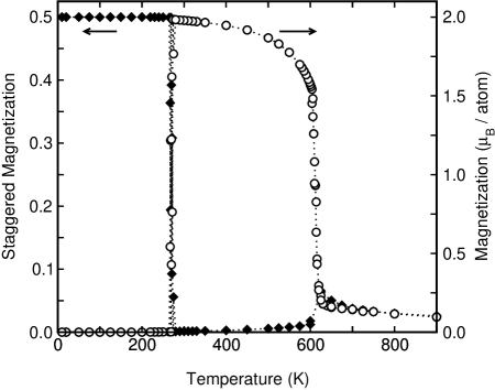
Figure 3: AF order parameter (diamonds) and magnetization (circles) as a function of temperature. The magnetization is obtained by multiplying the spin values with a value of $3.0\,\mu_{\rm B}$ for Fe and $1.0\,\mu_{\rm B}$ for Rh before averaging. The simulated system size is $L=10$.

Figure 4: Mean magnetic moment of the Rh atoms.

The order parameter of the AF phase is the staggered magnetization for the AF-II spin structure, i. e. the sum (of the absolute values) of the staggered magnetizations of the two simple cubic sublattices that constitute the bcc lattice structure. The staggered magnetization of a simple cubic (NaCl) lattice is defined as sum of spins multiplied with a sign which alternates depending on whether the corresponding spin occupies a Na or a Cl position. The order parameter of the FM phase is given by the magnetization of the lattice. The variation of both order parameters with temperature is shown in Fig. 3 for a system of size $L=10$. At low temperatures the staggered magnetization approaches a maximum value of $0.5$ due to the fact that the Rh sublattice has no moment (Fig. 4) and therefore does not contribute to the sum. At $T_{\rm m}=268\,$K the staggered magnetization abruptly drops to zero, whereas magnetic moment and magnetization increase close to their saturation values. Above $T_{\rm C}=610\,$K ferromagnetism breaks down and the system becomes paramagnetic. At the same time, the average moment of the Rh atoms falls down to a value of $0.2\,\mu_{\rm B}$. This is also the reason, why the decrease in the magnetization appears unusually sharp. From the data, a phase transition of second as well as of first order seems to be possible. Accordingly, it is known that for negative values of $D$ the Blume-Capel model can show both kinds of phase transitions separated by a tricritical point in the $T$-$D$-plane.Blume et al. (1971); Saul et al. (1974); Jain and Landau (1980) Hence in order to safely determine the nature of this phase transition further calculations are necessary.

A close look at the specific heat (Fig. 5) helps to explain the occurrence of a metamagnetic transition. At first sight it seems as if the specific heats of FM and AF phases do not differ very much below $350\,$K. Above this temperature the specific heat of the AF phase increases more rapidly with temperature until around $570\,$K the overheated AF phase is not stable anymore in the simulations and transforms to the FM phase. However, the inset shows that starting around $100\,$K the specific heat of the FM phase is enhanced compared to the AF heat. We explain this enhancement by a Schottky-type anomaly which adds up to the excitations from spin flips. Schottky anomalies are observed in systems with two levels separated by a small energy barrier. In fact a crossover from magnetic to nonmagnetic Rh atoms is conform with this picture. In the FM phase the Rh atoms have a moment being ferromagnetically aligned to the Fe moments, because the loss of the moment would correspond to an energy loss of eight times the exchange constant. This amount is diminished by the energy gain due to the $D_{\rm Rh}$ term, which is smaller than $8\times J^{\rm nn}_{\rm FeRh}$ but larger than $4\times J^{\rm nn}_{\rm FeRh}$, since the ground state is otherwise not antiferromagnetic. Increasing fluctuations of the magnetization of the Fe sublattice cause this energy difference to decrease and finally lead to a breakdown of the average Rh moment at $T_{\rm C}$. In the AF phase magnetic Rh atoms can be excited at the expense of the energy $D_{\rm Rh}$. There is, however, no gain in energy due to the exchange interaction, since the contributions from the AF Fe atoms cancel at the Rh site. This corresponds to a much larger energy difference between magnetic and nonmagnetic Rh states compared to the FM phase and does not lead to an appreciable contribution to the specific heat.

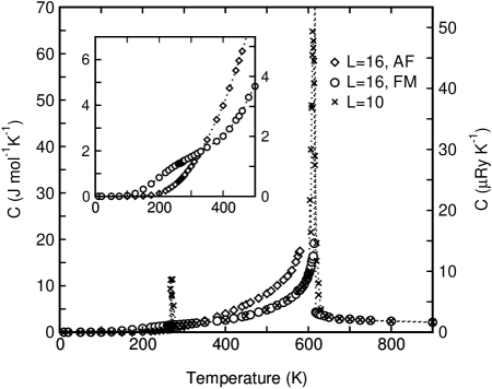
Figure 5: Specific heat as a function of temperature for the FM and the AF phases ($L=16$) and for simulations on smaller lattices using the global MC step ($L=10$). Inset: The specific heat of the AF and FM phase between $0$ and $500\,$K. Clearly visible is a Schottky-type enhancement below $300\,$K in the FM phase, which is responsible for the metamagnetic transition. The sharp peak around $270\,$K corresponds to the metamagnetic transition, which is observed in the small system due to the global MC step.

Figure 6: Free energy of the FM and AF phases obtained by integrating $C/T$, with the transition point at $T_{\rm m}=266\,$K.

This view is further supported by a comparison of the free energy of both phases shown in Fig. 6: The curves intersect at $T\approx 266\,$K, which is in excellent agreement with the simulated $T_{\rm m}=268\,$K. This accuracy could be achieved, because the data for the specific heat obtained from the simulations have only little spread and the fitted curves interpolate the data points perfectly. From the difference between the internal energies of both phases at the transition point, the entropy jump at $T_{\rm m}$ is determined to $\Delta S(T_{\rm m})=5.2\,{\rm J\,Kg^{-1}K^{-1}}$, which is only $30$ to $45\,\%$ of the experimental values (but of the right order of magnitude). But, one has to bear in mind that with the choice of an Ising model we neglected the possibility of non-collinear moments. For the Rh moments this can only occur in the FM phase, and would therefore contribute to $\Delta S(T_{\rm m})$. A second point is that the weight of the $S_{i}=0$ state is the same as for each magnetic state $S_{i}=\pm 1$. This is a natural choice for the spin-1 Ising model; but for the real system this is somehow arbitrary, because we have no information about the electronic origin of both Rh states.

IV An extended model

Since the simple spin Hamiltonian (1) can reproduce a metamagnetic transition as observed in $\alpha$-FeRh, it remains an interesting question whether other outstanding properties of this alloy, as the large volume increase at $T_{\rm m}$, can also be explained. Furthermore, it has still to be proven whether our spin analogy is a good approximation to the ab initio results in the sense that it has comparable low temperature properties. In order to check this we have to extend (1) for a description of elastic and magneto-volume properties:

$$H = -\,\sum_{i}^{~{}}\>D_{i}\>S_{i}^{2}-\!\!\!\sum_{<{\rm nn,nnn}>}\!\!\!J_{ik}(r_{ik})\>S_{i}\>S_{k}$$ (3)

$$+\sum_{<{\rm nn}>}\!\!V_{\rm nn}(r_{ik})+\!\!\sum_{<{\rm nnn}>}\!\!V_{\rm nnn}(r_{ik})\>.$$

For $V(r_{ik})$ we use simple pair potentials of the Lennard-Jones type:

$$V(r_{ik})=4\>\epsilon\left[\left(\frac{\sigma}{r_{ik}}\right)^{12}-\left(\frac{\sigma}{r_{ik}}\right)^{6}\right]\>.$$ (4)

Since in general the lattice structure of a Lennard-Jones system is closely packed, two different pair potentials for nearest and next-nearest neighbors have to be used in order to stabilize the bcc structure. The potentials, however, do neither distinguish between different atom types nor between the different spin states, as has been done in previous simulations of related materials like Fe-Ni Invar or Y(Mn_xAl_1-x)₂.Gruner et al. (1998); Gruner and Entel (2002) The use of Lennard-Jones potentials is far from being optimum for metals, but has numerical advantages that enable us to speed up the calculations substantially. It is then sufficient to choose the parameters so that basic elastic properties like low temperature lattice constant, bulk modulus or thermal expansion are reproduced.

Another change compared to (1) is that the exchange parameter is now taken to be a function of interatomic distance. For simplicity, we assume a linear distance dependence:

$$J_{ik}(r_{ik})=J_{ik}+\frac{\partial J_{ik}}{\partial r}\>r_{ik}\>.$$ (5)

The values for $J_{ik}$ which we take in the extended calculations are roughly the same as in Table 2. The relation between the derivatives of $J^{\rm nn}_{\rm FeRh}$ and $J^{\rm nnn}_{\rm FeFe}$ with respect to the interatomic distance was determined by the relation of the pressure derivatives of the Curie and Néel temperatures, respectively, which have been obtained from the experimental phase diagram by assuming a linear dependence between $\partial J_{ik}/\partial r$ and $\partial T_{\rm C,N}/\partial p$. The absolute values have been adapted to reproduce the volume jump at $T_{\rm m}$. An exchange interaction of this form has also been used to describe magneto-volume effects in Fe-Ni Invar.Grossmann and Rancourt (1996); Rancourt and Dang (1996); Lagarec and Rancourt (2000) In this case, the derivative of the exchange constant $\partial J_{ik}/\partial r$ was a factor of $2$ to $20$ larger than in the present work. The values of parameters are summarized in Table 3.

$D_{\rm Fe}$	$D_{\rm Rh}$	$J^{\rm nn}_{\rm FeRh}({2.6\>{\rm\AA}})$	$J^{\rm nnn}_{\rm FeFe}({3.0\>{\rm\AA}})$	$J^{\rm nnn}_{\rm RhRh}({3.0\>{\rm\AA}})$
$\gg\!k_{\rm B}\,T$	$-11.1$	$2.10$	$-1.04$	$0$
		$\partial J^{\rm nn}_{\rm FeRh}/\partial r$	$\partial J^{\rm nnn}_{\rm FeFe}/\partial r$	$\partial J^{\rm nnn}_{\rm RhRh}/\partial r$
		$1.97$	$1.58$	$0$
	$\epsilon_{\rm nn}$	$\sigma_{\rm nn}$	$\epsilon_{\rm nnn}$	$\sigma_{\rm nnn}$
	$25.23$	$2.32$	$25.23$	$2.67$

Table 3: Magnetic and elastic parameters for the extended spin model (energies in mRy, distances in $\rm\AA$).

IV.1 Details of computation

For the evaluation of Hamiltonian (3) we use a textbook isothermal-isobaric Monte Carlo method (e. g. Ref. Allen and Tildesley, 1987) consisting of alternating spin and position updates for each atom and a global volume update step after finishing each lattice sweep. This algorithm has been used by the the authors in previous calculations and is explained in detail in the corresponding references.Gruner et al. (1998); Gruner and Entel (1998, 2002) In order to simulate the metamagnetic transition, an additional global spin update step has to be introduced. We use the same algorithm as described in the last section for the spin system in connection with a simultaneous volume adaption. Since the latter reduces the acceptance probability considerably, the global update scheme has to be repeated several thousands of times. It is not practicable to use a new spin configuration for each trial step, because the evaluation of the energy is comparatively time consuming. On the other hand, the new energy after solely rescaling the volume can be calculated very quickly, since due to the use of Lennard-Jones potentials the energy can be written as a function of integral powers of the lattice parameter. Therefore, we choose a trial spin configuration as described before and compute the new energy. Then we attempt a previously fixed number $N$ of Metropolis steps, each with a newly chosen volume. If one step is accepted, we continue with the original spin configuration as trial system (and so on) until $N$ steps have been made. Since the number of trial steps $N$ has been previously fixed, detailed balance is still valid.

We have performed simulations with system sizes of $L=6$ to $12$. A direct metamagnetic transition could only be seen for system sizes up to $L=8$. The simulation time ranged from $120\,000$ up to $1\,000\,000$ lattice sweeps around $T_{\rm m}$ with values from $1000$ to $10\,000$ for $N$. As before we estimated Gibbs’ free energy for zero pressure by integrating the specific heat according to Eq. (2).

IV.2 Computational results

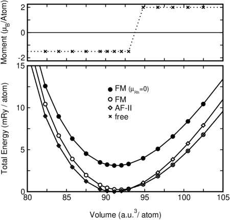
Figure 7: Internal energy and moment as a function of the atomic volume obtained for Hamiltonian (3) at $T=4\,$K. The simulations have been performed for fixed spin structures as well as for a freely relaxed spin system.

For a comparison of our model properties with the results of ab initio calculations, we calculated in isochoric simulations the energy as a function of the volume at low temperatures for different fixed spin structures (Fig. 7). Here, we cooled a system of size $L=16$ exponentially down from $100\,$K down to $4\,$K. We find good agreement with the results of Fig. 2 in the sense that the order of magnetic phases is similar. Although the ab initio total energy differences are somewhat larger, this indicates that our model Hamiltonian (3) is a qualitatively correct description of the mechanisms leading to a metamagnetic transition in FeRh.

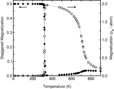
Figure 8: AF order parameter (diamonds) and magnetization (circles) as a function of temperature as obtained for the extended model Hamiltonian (3). The system size is $L=8$.

Figure 9: Mean magnetic moment of the Rh atoms for the extended model ($L=8$).

As in the simple model without volume-dependent terms, we find an abrupt increase of the magnetization in combination with a discontinuous decrease for the staggered magnetization with increasing temperature (Fig. 8). Consequently the mean moment at the Rh sites (Fig. 9) also raises sharply around the metamagnetic transition temperature of $T_{\rm m}=322\,$K. Around the Curie temperature $T=720\,$K the magnetization decreases more smoothly than for the simple model. This may be due to the enhancement of the effective exchange parameter given by Eq. (5) which is caused by the lattice expansion.

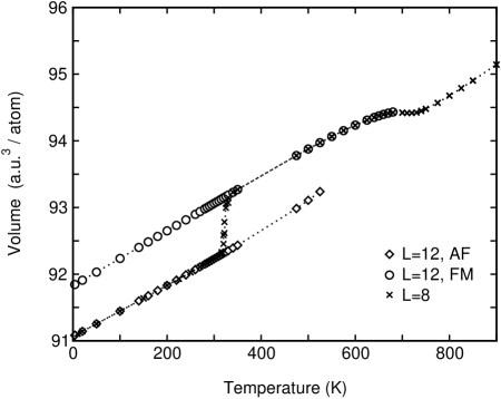
Figure 10: Volume per atom plotted over temperature as obtained for the AF and FM phases ($L=12$) and by our simulations with the global update scheme ($L=8$).

As expected from the low temperature calculations, the volume of the AF phase is smaller than the volume of the FM phase throughout the stability range (Fig. 10). For the freely fluctuating system a volume jump of $0.8\,\%$ occurs at $T_{\rm m}$. Below $T_{\rm C}$ the volume expansion is reduced in the FM phase, which is in qualitative agreement with experimentZakharov et al. (1964); Aigarabel et al. (1996).

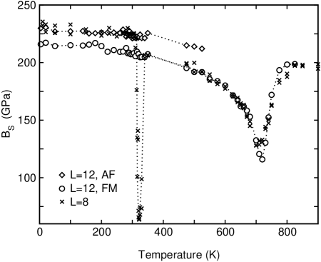
Figure 11: Adiabatic bulk modulus as a function of temperature for the AF and FM phases ($L=12$) and with the global update scheme ($L=8$). The latter data, which show the metamagnetic transition, reveal a very large softening of the lattice around $T_{\rm m}$.

The bulk modulus $B_{\rm S}$ of the AF phase is about $6\,\%$ larger than the FM bulk modulus throughout the stability range (Fig. 11). Around $T_{\rm m}$ and $T_{\rm C}$ we find a considerable weakening of the material which is caused by the magneto-volume anomalies. The values for $B_{\rm S}$ at low temperatures can be estimated more accurately by using a polynomial fit to the $E$-$V$ curves in Fig. 7. We find $B_{\rm S}=231\,$GPa for the AF phase and $B_{\rm S}=217\,$GPa for the FM phase. These values are in good agreement with results of isobaric calculations shown in Fig. 11. Compared with the results of ab initio calculations (Table 1) the absolute values are too large, whereas these calculations do not give a unanimous prediction for the sign and the magnitude of the difference $\Delta B_{\rm S}$ (with respect to the magnetic structures). Experimental measurementsZakharov et al. (1964) of Young modulus suggest that the bulk modulus of the AF phase should in fact be lower than in the FM phase. The modulus of the AF phase, however, has only been estimated in the vicinity of $T_{\rm m}$, where a weakening of the material (as a precursor of the transition) is present (as in our simulations).

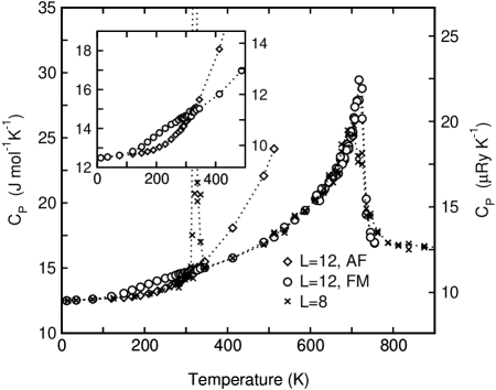
Figure 12: Specific heat for the extended model as a function of temperature for FM and the AF phases ($L=12$) and for simulations on smaller lattices using the global MC step ($L=8$). The relationship between the specific heats of AF and FM phases below $400\,$K is shown in the inset.

The specific heats obtained for the extended model (Fig. 12) resemble the findings for the spin-only Hamiltonian (1), except that now additional contributions due to atomic displacements are included. This shows that the proposed explanation of the metamagnetic transition is still valid. Since the Hamiltonian (3) does not contain any kinetic terms, the low temperature value of the specific heat is only half of the Dulong-Petit limit of $3\,R$, where $R$ is the kinetic gas constant.

IV.3 Estimation of Gibbs free energy

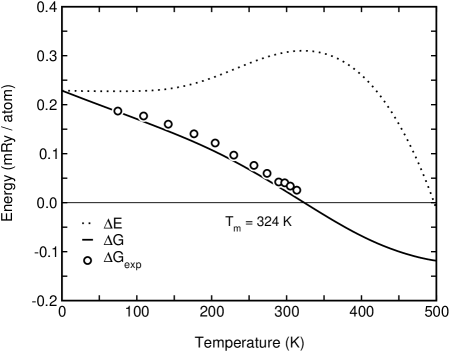
Figure 13: Differences of internal energies and Gibbs free energies for FM and AF phases obtained by integrating $C_{\rm p}/T$. The transition point is $T_{\rm m}=324\,$K. The experimental data have been obtained by integrating over the hysteresis loop for different temperatures.Ponomarev (1972)

The calculation of Gibbs free energy $G$ for the model with classical motion (3) is more complicated than in the spin-only case (1). First of all absolute values of $G$ cannot be given, since the specific heat at zero temperature is finite and the resulting entropy would diverge. But since the limit for $T$ $\to$ $0$ of $C_{\rm p}$ is $1.5\,R$ and hence the same for all magnetic structures, differences of free energies can be computed. In contrast to the previous section, the entropy contribution at zero temperature $\Delta S(0)$ must be considered. As before a contribution from the magnetic system can be neglected, while we have to account for the differences in the elastic properties of FM and the AF phases. Since we only need the entropy at zero temperature, we choose an ensemble of harmonic oscillators as an approximation for our spatial degrees of freedom, neglecting the anharmonicity of the potentials and the coupling of the oscillators. Differentiating the free energy obtained from the logarithm of the partition function leads then to a simple expression for the entropy difference,

$$\Delta S=\frac{3}{2}Nk_{\rm B}\ln\left(k_{\rm AF}/k_{\rm FM}\right)\>,$$ (6)

where $k_{\rm AF}$ and $k_{\rm FM}$ are the force constants of the harmonic potentials which are estimated from the curvature of the ground state energy (versus lattice parameter) curve. For the entropy difference we obtain then: $\Delta S(0)=9.17\,{\rm J\,kg}^{-1}{\rm K}^{-1}$. Taking this into account, we achieve again a rather good value for $T_{\rm m}$. From the differences of internal energies at $T_{\rm m}$ we obtain for the entropy jump at the transition $\Delta S(T_{\rm m})=15.9\,{\rm J\,kg}^{-1}{\rm K}^{-1}$, which is within the range of experimental results. Comparison of the calculated free energy with experimental values for $\Delta G$ shows excellent agreement. The experimental values have been obtained by a graphical integration of the magnetic field expressed as a function of the measured magnetization.Ponomarev (1972) Extrapolation of experimental values to zero temperature shows that the energy difference $\Delta E(0)$ between the AF and FM phases is much better described by our model parameters than by ab initio results, since the latter show that $\Delta E$ is one order of magnitude too large. This discrepancy has already been noticed by Moruzzi and MarcusMoruzzi and Marcus (1992b) who relate this to the omission of zero point energy corrections in their total energy calculations.

V Conclusions

We propose on the basis of new ab initio results a mechanism for the metamagnetic transition in FeRh at finite temperatures. In contrast to previous explanations, our model does not rely on a large difference between the low temperature specific heat constants of both phases. These are expected to be sensitive to external influences as both experimental measurements and band structure calculations suggest, so that it seems implausible that a constant contribution of the given magnitude might survive up to room temperature. Instead, we propose that the existence of two magnetic states of Rh atoms connected with competing FM Fe-Rh and AF Fe-Fe exchange interactions are at the origin of the metamagnetic transition. The magneto-volume effects can simply be explained on the basis of distance dependent exchange parameters. The applicability of this mechanism to the Fe-Rh problem has been verified by Monte Carlo model calculations, showing that a metamagnetic transition of the desired kind does in fact occur and, by extending the model, magneto-volume effects and other experimental properties can be sufficiently well described.

As we have pointed out, our explanation is in agreement with existing experimental data. However, a further check of our model would be a comparison with (non-existing) specific heat data from above $T_{\rm C}$ down to very low temperatures for both, the AF and FM phases. From this one could then estimate the magnetic contribution by subtracting the lattice part within the Debye approximation, the electronic part and the contribution by the anharmonicity of the potentials.Bendick et al. (1978); Rellinghaus et al. (1995) So far, the specific heat has only been determined in the range from $100\,$K to $500\,$K and only for the nearly stoichiometric Rh-rich alloy.Richardson et al. (1973); Annaorazov et al. (1992) Systematic measurements on the Fe-rich side with a FM ground state and measurements under pressure, suppressing the metamagnetic transition would yield information whether a Schottky-type excitation plays an important role, which should show up around $200\,$K in the magnetic contribution to the specific heat of ferromagnetic samples.

Monte Carlo simulations with applied pressure are left for future work, since with increasing pressure and hence increasing $T_{\rm m}$ a reliable estimation of the transition temperature is rather difficult and requires an improvement of the global MC step. First tests, however, showed that the location of the phase boundaries under pressure is in sufficient agreement with experimental data for pressures below $20\,$kbar and above $40\,$kbar, where the metamagnetic transition is completely suppressed. The tricritical point, if one exists, should be located somewhere between $20\,$kbar and $40\,$kbar for the parameters used here.