Dilute limit of a strongly-interacting model of spinless fermions and hardcore bosons on the square lattice

Abstract

In our model, spinless fermions (or hardcore bosons) on a square lattice hop to nearest neighbor sites, and also experience a hard-core repulsion at the nearest neighbor separation. This is the simplest model of correlated electrons and is more tractable for exact diagonalization than the Hubbard model. We study systematically the dilute limit of this model by a combination of analytical and several numerical approaches: the two-particle problem using lattice Green functions and the t-matrix, the few-fermion problem using a modified t-matrix (demonstrating that the interaction energy is well captured by pairwise terms), and for bosons the fitting of the energy as a function of density to Schick’s analytical result for dilute hard disks. We present the first systematic study for a strongly-interacting lattice model of the t-matrix, which appears as the central object in older theories of the existence of a two-dimensional Fermi liquid for dilute fermions with strong interactions. For our model, we can (Lanczos) diagonalize the $7\times 7$ system at all fillings and the $20\times 20$ system with four particles, thus going far beyond previous diagonalization works on the Hubbard model.

I introduction

Since the discovery of the high-temperature superconductors in 1986, there has been intense study of a number of two-dimensional models that are believed to model the electronic properties of the CuO₂ plane of the cuprate superconductors, for example, the Hubbard model, the $t-J$ model, and the Heisenberg model.Dagotto ; Manou Two-dimensional quantum models with short-range kinetic and interaction terms are difficult to study. In one dimension, there are exact solutions using the Bethe ansatz and a host of related analytical techniques,LiebMattis and there is a very accurate numerical method, the density-matrix renormalization group (DMRG),dmrg that can be applied to large systems relatively easily. In two dimensions, on the other hand, there are few exact solutions (one famous nontrivial case is the Hubbard model with one hole in a half-filled background, the Nagaoka stateNagaoka ), and current numerical methods are not satisfactory (quantum Monte Carlo is plagued by the negative sign problemDagotto at low temperatures and at many fillings of interest and the DMRG in two dimensions2Ddmrg is still in early development stage).

The most reliable method for studying complicated quantum systems is exact diagonalization, which means enumerating all basis states and diagonalizing the resulting Hamiltonian matrix. Of course, this method is computationally limited by the growth of the Hilbert space which is in general exponential in the number of particles and the lattice size. The $4\times 4$ Hubbard model with 16 electrons, 8 spin-up and 8 spin-down, after reduction by particle conservation, translation, and the symmetries of the square, has 1,310,242 states in the largest matrix block,Lin and can be diagonalized using the well-known Lanczos method. The Hubbard model has been diagonalized for the $4\times 4$ lattice (see e.g., Ref. Fano, ), and at low filling (four electrons) for $6\times 6$Bruus with extensive employment of symmetries.

I.1 The spinless fermion model

We have asked the question: Is there a model that contains the basic ingredient of short-range hopping and interaction but is simpler, in the exact diagonalization sense, than the Hubbard model? The answer is yes: we can neglect the spin. We obtain the following Hamiltonian for spinless fermions,

$$H=-t\sum_{\langle i,j\rangle}\left(c^{\dagger}_{i}c_{j}+c^{\dagger}_{j}c_{i}\right)+V\sum_{\langle i,j\rangle}\hat{n}_{i}\hat{n}_{j},$$ (1)

where $c^{\dagger}_{i}$ and $c_{i}$ are spinless fermion creation and annihilation operators at site $i$, $\hat{n}_{i}=c^{\dagger}_{i}c_{i}$ the number operator, $t$ the nearest-neighbor hopping amplitude, and $V$ the nearest-neighbor interaction. Note that with spinless fermions, there can be at the most one particle per site; no on-site interaction (as that in the Hubbard model) is possible, and we have included in our Hamiltonian nearest-neighbor repulsion.

The spinless fermion model, Eq. (1), is a two-state model, and the number of basis states for a $N$-site system is $2^{N}$, which is a significant reduction from the $4^{N}$ of the Hubbard model. We can further reduce the number of basis states by taking the nearest-neighbor interaction $V=+\infty$, i.e., infinite repulsion, which excludes nearest neighbors, giving roughly $2^{N/2}$ states.

The spinless fermion model with infinite repulsion Eq. (1) contains a significant reduction of the Hilbert space. After using particle conservation and translation symmetry (but not point group symmetry), the largest matrix for the $7\times 7$ system has $1,906,532$ states (for 11 particles), and we can therefore compute for all fillings the $7\times 7$ system whereas for the Hubbard model $4\times 4$ is basically the limit. This of course means that for certain limits we can also go much further than the Hubbard model, for example, we can handle four particles on a $20\times 20$ lattice where the number of basis states is $2,472,147$. This extended capability with our model has enabled us to obtain a number of results that are difficult to obtain with the Hubbard model.

An added feature of our model is that the basis set for the spinless fermion problem is identical to that for the hardcore boson problem, because with hardcore repulsion, there can be at the most one boson at one site also. Therefore, without computational difficulty, we can study numerically both the spinless fermion and hardcore boson problem.

Spinless fermions can also be realized in experiments, for example, the spin polarized ³He due to a strong magnetic field, or ferro or ferri-magnetic electronic systems where one spin-band is filled. The one-dimensional spinless fermion model with finite repulsion is solved exactly using Bethe ansatz.YangYang The infinite-dimensional problem is studied in Ref. Uhrig, . A very different approach using the renormalization group for fermions is done in Ref. Shankar, . A Monte Carlo study of the two-dimensional model at half-filling only and low temperatures is in Ref. Guber, , which, dating back to 1985, is one of the earliest quantum Monte Carlo simulations for fermions. (It is no coincidence that they chose the model with the smallest Hilbert space.)

Considering the tremendous effort that has been devoted to the Hubbard model and the close resemblance of our model, Eq. (1), to the Hubbard model, it is surprising that works on this spinless model have been rather sparse, though it has been commented that the spinless model offers considerable simplifications.VollFermi

This paper is one of the two that we are publishing to study systematically the two-dimensional spinless fermion and hardcore boson model with infinite nearest-neighbor repulsion. The present paper focuses on the dilute limit, treating the problem of a few particles, and the other paperstripepaper will focus on the dense limit, near half-filled,FN-halffilled where stripes (that are holes lining up across the lattice) are natural objects (see Ref. HenleyZhang, for a condensed study of stripes in this model). We will use Lanczos exact diagonalization, exploiting the much-reduced Hilbert space of our model, and a number of analytical techniques, for example, in this paper, lattice Green functions and the t-matrix. One of the goals of these two papers is to advertise this model of spinless fermions to the strongly-correlated electron community, as we believe that it is the simplest model of correlated fermions and deserves more research effort and better understanding.

The prior work most comparable to ours may be the studies of four spinless electrons in a $6\times 6$ lattice, with Coulomb repulsion, by Pichard et al; Pichard their motivation was the Wigner crystal melting and the competition of Coulomb interactions with Anderson localization when a disorder potential is turned on.

I.2 The t-matrix

At the dilute limit of our model, the scattering t-matrix is of fundamental importance. For two particles, we expect that, at least when the potential $V$ is small, we can write a perturbative equation for energy,

$$E={\cal E}({\bf q}_{1})+{\cal E}({\bf q}_{2})+\Delta E({\bf q}_{1},{\bf q}_{2}),$$ (2)

which is to say that the exact interacting energy of two particles is the noninteracting energy ${\cal E}({\bf q}_{1})+{\cal E}({\bf q}_{2})$, for a pair of momenta ${\bf q}_{1}$ and ${\bf q}_{2}$, plus a correction term $\Delta E$ due to the interaction $V$. And with more than two particles, at least when the particle density is low, we expect to have

$$E=\sum_{\bf q}{\cal E}({\bf q})+\frac{1}{2}\sum_{{\bf q},{\bf q}^{\prime}}\Delta E({\bf q},{\bf q}^{\prime}).$$ (3)

Eq. (3) is central in Fermi liquid theory, where it is justified by the so-called “adiabatic continuation” idea, which says that interacting fermion states correspond one-to-one to noninteracting ones as we slowly switch on a potential.

In the boson case, because many bosons can occupy one quantum mechanical state and form a condensate, Eq. (3) should be modified, but with only two bosons, we expect Eq. (2) should be valid (in that the correction vanishes in the dilute limit). Eqs. (2) and (3) are used when we look at a list of noninteracting energies and draw correspondences with the interacting energies, the energy shift being packaged in the term $\Delta E$.

One possible objection to the above formulas (Eqs. (2) and (3)) is that they appear to be perturbative, yet the interaction potential in our problem is infinitely strong, so the first-order (first Born approximation) scattering amplitude, being proportional to the potential, is infinite too. However, this singular potential scattering problem (e.g., hard-sphere interaction in 3D) has been solved (see Ref. Landau, ) by replacing the potential with the so-called scattering length, which is finite even when the potential is infinite. As we review in Appendix B, a perturbation series (Born series) can be written down (that corresponds to a series of the so-called ladder diagrams) and even though each term is proportional to the potential, the sum of all terms (the t-matrix, $\Delta E$ in Eqs. (2) and (3)) is finite.

Because the t-matrix captures two-body interaction effects, it is the centerpiece of dilute fermion and boson calculations with strong interactions. Field-theoretical calculations in both three and two dimensions are based on the ladder diagrams and the t-matrix. See Fetter and WaleckaFetter for the 3D problem, SchickSchick for the 2D boson problem and BloomBloom the 2D fermion problem. For lattice fermion problems, KanamoriKanamori derived the t-matrix for a tight-binding model that is essentially a Hubbard model (this work is also described in YosidaYosida ). And in Ref. Mattis, , the t-matrix is worked out explicitly for the Hubbard model, and Kanamori’s result is obtained. Ref. Mattis, also evaluated the t-matrix for the dilute limit in three dimensions and obtained a functional dependence on particle density.

Rudin and MattisRudinMattis used the t-matrix expression derived in Refs. Kanamori, and Mattis, and found upper and lower bounds of the fermion t-matrix in two dimensions in terms of particle density. Rudin and Mattis’s result for the low-density limit of the two-dimensional Hubbard model is of the same functional form as Bloom’s diagrammatical calculation for the two-dimensional fermion hard disks.Bloom Since the discovery of high-temperature superconductors, Bloom’s calculation has received a lot of attention because of its relevance to the validity of the Fermi liquid description of dilute fermions in two dimensions. There have been a number of works on the 2D dilute Fermi gasEngel1 ; Engel2 ; Engel3 and on the dilute limit of 2D Hubbard model,FukuHubbard all using the t-matrix, but these results have not been checked by numerical calculations.

In fact, we are not aware of a systematic study of the t-matrix for a lattice model. In this paper, we present the first such study for the two-particle problem in Sec. III (for bosons and fermions) and the few-fermion problem in Sec. IV. We check the t-matrix results with exact diagonalization data and show that our t-matrix on a lattice is the sum of the two-body scattering terms to infinite order.

I.3 Paper organization

In this paper, we will study systematically the dilute limit of our model Eq. (1), focusing on the problem of a few particles. Our paper is divided into four parts.

In Sec. II, the two-particle (boson and fermion) problem is studied. We formulated the two-particle Schrodinger equation using lattice Green functions, employ some of its recursion relations to simplify the problem, and obtain the two-boson ground state energy in the large-lattice limit. Using the two-particle result, we then study the problem of a few particles and obtain an expression for ground state energy on a large lattice.

In Sec. III, the two-particle problem is then cast into a different form, emphasizing the scatterings between the two particles. The result is the t-matrix, that is exact for the two-particle problem and contains all two-body scattering terms. We will study the two-particle t-matrix in great detail, showing the differences between the boson and fermion cases, and demonstrating that the first t-matrix iteration is often a good approximation for fermion energy. In Appendix B, we show explicitly that the t-matrix we obtain is the sum total of all two-body scattering terms.

The problem of a few fermions is taken up in Sec. IV. First, the fermion shell effect is discussed and demonstrated from diagonalization, and we show the difference for bosons and fermions. We show the modifications to the two-fermion t-matrix that enable us to calculate energies for three, four, and five particles. Using this t-matrix, we can compute the interaction corrections to the noninteracting energy and trace the change in the energy spectrum from the nointeracting one to the interacting one.

Finally, in Sec. V, we discuss the energy per particle curve for dilute bosons and fermions. We have studied the two-dimensional results derived by SchickSchick for bosons and BloomBloom for fermions by fitting the data from diagonalization for a number of lattices. Schick’s result for dilute bosons is checked nicely, and we explain that for spinless fermions in our model we will need the p-wave scattering term, which is not included in Bloom’s calculation.

In Appendix A, we discuss briefly our exact diagonalization computer program, which can handle arbitary periodic boundaries specified by two vectors on the square lattice and uses translation symmetry to reduce the matrix size.

II The Two-Particle Problem

The two-particle problem has appeared in many different contexts. The most familiar one is the hydrogen atom problem in introductory quantum mechanics textbooks. The two-magnon problem is closely related mathematically to our two-particle problem, and it has been solved in arbitary dimensions for ferromagnets (see e.g., Ref. Mattis, ). Another important two-particle problem is the Cooper problem, with two electrons in the presence of a Fermi sea (see e.g., Ref. Baym, ). And motivated by the possibility of Cooper pair formation in high-temperature superconductors, there have also been a number of studies on bound states on a two-dimensional lattice.Yang ; Hirsch ; Lin91 ; Petukhov ; Blaer ; Leung01 The two-electron problem in the plain two-dimensional repulsive Hubbard model is studied in Ref. Fabrizio, , and ground state energy in the large-lattice limit is obtained analytically.

In this section, we present a rather complete calculation for the two-particle problem in our model, treating both bosons and fermions. With infinite repulsive interaction in our model, we are not interested in finding bound states. We calculate eigenenergies for all states for a finite-size lattice, and our calculation is more complicated than the Hubbard modelFabrizio case because of nearest-neighbor (in place of on-site) interaction. Where the Green function in the Hubbard case was a scalar object, in our case it is replaced by a $4\times 4$ matrix, corresponding to the four nearest neighbor sites where the potential acts. This Green function study of the two-particle problem is closely related to the treatment of the two-electron problem in the Hubbard modelFabrizio and that in an extended Hubbard model.Blaer We will show the use of lattice symmetry and recursion relations to simplify the problem with nearest-neighbor interactions.

II.1 Preliminary

In this two-particle calculation, we will work in momentum space, and we will start with a Hamiltonian more general than Eq. (1),Blaer

$$H=T+U,$$ (4)

$$T=\sum_{{\bf r}_{1}{\bf r}_{2}}t({\bf r}_{2}-{\bf r}_{1})c_{{\bf r}_{1}}^{\dagger}c_{{\bf r}_{2}},$$ (6)

$$U=\sum_{{\bf r}_{1}{\bf r}_{2}}V({\bf r}_{2}-{\bf r}_{1})c_{{\bf r}_{1}}^{\dagger}c_{{\bf r}_{1}}c_{{\bf r}_{2}}^{\dagger}c_{{\bf r}_{2}}.$$

Here we have allowed hopping and interaction between any two lattice sites, but we require that both depend only on the separation between the two vectors and both have inversion symmetry. That is $t({\bf r}_{1},{\bf r}_{2})=t({\bf r}_{2}-{\bf r}_{1})$, $t(-{\bf r})=t({\bf r})$, $V({\bf r}_{1},{\bf r}_{2})=V({\bf r}_{2}-{\bf r}_{1})$, and $V(-{\bf r})=V({\bf r})$. In momentum space, Eqs. (6) and (6) become,

$$T=\sum_{\bf p}{\cal E}({\bf p})c_{\bf p}^{\dagger}c_{\bf p},$$ (7)

$$U=\frac{1}{2N}\sum_{{\bf p}{\bf p}^{\prime}{\bf k}}V({\bf k})c_{\bf p}^{\dagger}c_{{\bf p}^{\prime}}^{\dagger}c_{{\bf p}^{\prime}+{\bf k}}c_{{\bf p}-{\bf k}},$$ (8)

where

$${\cal E}({\bf p})=\sum_{\bf r}t({\bf r})e^{i{\bf p}{\bf r}},$$ (9)

$$V({\bf k})=\sum_{\bf r}V({\bf r})e^{i{\bf k}{\bf r}},$$ (10)

with ${\cal E}(-{\bf p})={\cal E}({\bf p})$ and $V(-{\bf k})=V({\bf k})$. Eqs. (6) and (6) reduce to our nearest-neighbor Hamiltonian Eq. (1) if we take,

$$t({\bf r})=\cases{-t,&${\bf r}=(\pm 1,0)(0,\pm 1)$,\cr 0,&otherwise,}$$ (11)

$$V({\bf r})=\cases{V,&${\bf r}=(\pm 1,0)(0,\pm 1)$,\cr 0,&otherwise,}$$ (12)

where we have taken the lattice constant to be unity,FN-notation and the nearest-neighbor vectors will be called

$${{\bf R}_{1}}=(1,0),{\bf R}_{2}=(-1,0),{\bf R}_{3}=(0,1),{\bf R}_{4}=(0,-1).$$ (13)

Then we have,

$${\cal E}({\bf p})=-2t(\cos p_{x}+\cos p_{y}),$$ (14)

$$V({\bf k})=2V(\cos k_{x}+\cos k_{y}).$$ (15)

Note that the structure of later equations depends sensitively on having four sites in Eq. (12) where $V({\bf r})\neq 0$m, but does not depend much on the form of Eq. (11) and the resulting dispersion Eq. (14).

Using momentum conservation of Eq. (4), the two-particle wave function that we will use is,

$$|\psi\rangle=\sum_{{\bf q}}g({\bf q})|{\bf q},{\bf P}-{\bf q}\rangle,$$ (16)

where the sum is over the whole Brillouin zone, and the coefficient $g({\bf q})$ satisfies,

$$g({\bf P}-{\bf q})={s_{bf}}g({\bf q}),$$ (17)

where ${s_{bf}}=1$ for bosons and $-1$ for fermions.

II.2 Green function equations

Applying the more general form of the Hamiltonian operator Eqs (7) and (8) to the state Eq. (16), the Schrodinger equation $(E-T)|\psi\rangle=U|\psi\rangle$ becomes

$$(E-{\cal E}({\bf q})-{\cal E}({\bf P}-{\bf q}))g({\bf q})=\frac{1}{N}\sum_{\bf k}V({\bf q}-{\bf k})g({\bf k}).$$ (18)

Eq. (18) is a matrix equation ${\cal A}g=Eg$ where ${\cal A}_{{\bf q}{\bf k}}=({\cal E}({\bf q})+{\cal E}({\bf P}-{\bf q}))\delta_{{\bf q}{\bf k}}+V({\bf q}-{\bf k})/N$. If $V$ is not infinity, this $N\times N$ matrix ${\cal A}$ can be diagonalized, and $E$ and $g({\bf q})$ are respectively the eigenvalue and eigenvector. To deal with $V=+\infty$, we need some further manipulations.

We consider the case when $E\neq{\cal E}({\bf q})+{\cal E}({\bf P}-{\bf q})$, for any ${\bf q}$, which is to say, the energy $E$ is not the energy of a noninteracting pair. The (lattice) Fourier transform of the coefficients $g({\bf q})$ is

$${\tilde{g}}({\bf r})=\sum_{\bf q}e^{-i{\bf q}\cdot{\bf r}}g({\bf q});$$ (19)

this is just the real-space wavefunction in terms of the relative coordinate ${\bf r}$. Define the lattice Green function,

$$G(E,{\bf P};{\bf r},{\bf r}^{\prime})=\frac{1}{N}\sum_{\bf q}\frac{e^{i{\bf q}\cdot({\bf r}^{\prime}-{\bf r})}}{E-{\cal E}({\bf q})-{\cal E}({\bf P}-{\bf q})},$$ (20)

then after dividing the first factor from both sides of our Schrodinger equation, Eq. (18), and Fourier transforming, we obtain

$${\tilde{g}}({\bf r})=\sum_{{\bf r}^{\prime}}G(E,{\bf P};{\bf r},{\bf r}^{\prime})V({\bf r}^{\prime}){\tilde{g}}({\bf r}^{\prime}).$$ (21)

In the following we return to the nearest-neighbor potential $V({\bf r})$ in Eq. (12). The Green function sum in Eq. (21) then has only four terms,

$${\tilde{g}}({\bf r})=\sum_{j}G(E,{\bf P};{\bf r},{\bf R}_{j})(V{\tilde{g}}({\bf R}_{j})),$$ (22)

summed over the separations in Eq. (13). If we also restrict ${\bf r}$ to the four nearest-neighbor vectors,FN-Blaer then Eq. (22) becomes,

$${\tilde{g}}({\bf R}_{i})=\sum_{j}G(E,{\bf P};{\bf R}_{i},{\bf R}_{j})(V{\tilde{g}}({\bf R}_{j})).$$ (23)

If we define the $4\times 4$ matrix,

$${\cal G}_{ij}(E,{\bf P})=G(E,{\bf P};{\bf R}_{i},{\bf R}_{j}),$$ (24)

and a $4\times 1$ vector ${\phi}_{j}={\tilde{g}}({\bf R}_{j})$, then we obtain a simple matrix equation,

$$(I-{\cal G}(E,{\bf P})V){\phi}=0.$$ (25)

We can also rewrite this equation as an equation for energy using the determinant,

$$\det(I-{\cal G}(E,{\bf P})V)=0.$$ (26)

With $V=+\infty$, we have even simpler equations

$${\cal G}(E,{\bf P})(V{\phi})=0,$$ (27)

and

$$\det{\cal G}(E,{\bf P})=0.$$ (28)

Notice we write $V\phi$ to denote the limit as $V\to\infty$; it would not do to write simply $\phi$ in Eqs. (25) and (27), since $\phi\to 0$ as $V\to\infty$ (being the amplitude of the relative wavefunction at the forbidden separations $\{{\bf R}_{i}\}$.).

For the Hubbard model, there is only on-site interaction, so $V({\bf r})$ is nonzero only when ${\bf r}=0$, and the sum in Eq. (21) has only one term. Eq. (23) is simply a scalar equation, which, after ${\tilde{g}}$ cancels from both sides of the equation and using Eq. (20), gives,

$$1=\frac{V}{N}\sum_{\bf q}\frac{1}{E-{\cal E}({\bf q})-{\cal E}({\bf P}-{\bf q})},$$ (29)

which is exactly the result in Ref. Fabrizio, .

II.2.1 Simplifications for rectangular boundaries

We specialize to the case of total momentum ${\bf P}=0$ and rectangular-boundary lattices. We have from Eqs. (20) and (24),

$${\cal G}_{ij}(E)=\frac{1}{N}\sum_{\bf q}\frac{\cos(q_{x}(R_{jx}-R_{ix}))\cos(q_{y}(R_{jy}-R_{iy}))}{E-2{\cal E}({\bf q})},$$ (30)

where the potential is nonzero on the sites $\{{\bf R}_{i}\}$ given by Eq. (13) and in the last step we have used the symmetry properties of the dispersion relation ${\cal E}(q_{x},q_{y})={\cal E}(q_{x},-q_{y})={\cal E}(-q_{x},q_{y})$. Obviously Eq. (30) is a function of displacements ${\bf R}_{j}-{\bf R}_{i}$, which (in view of Eq. (13) can be (0,0), (1,1), (2,0), or any vector related by square symmetry. It is convenient for this and later sections to define a new notation for the Green function ${\cal G}_{ij}$, emphasizing its dependence on ${\bf R}_{j}-{\bf R}_{i}=(m,n)$,

$$\Gamma(E,m,n)=\frac{1}{N}\sum_{\bf q}\frac{\cos(mq_{x})\cos(nq_{y})}{E+4\cos q_{x}+4\cos q_{y}},$$ (31)

where the sum is over the $N$ wavevectors ${\bf q}=(2\pi l_{x}/L_{x},2\pi l_{y}/L_{y})$ with $0\leq l_{x}<L_{x}$ and $0\leq l_{y}<L_{y}$ (for one Brillouin zone), and we have used the expression for ${\cal E}({\bf q})$ from Eq. (14) (and taken $t=1$).

This Green function for rectangular-boundary lattices satisfies the following reflection properties,

$$\Gamma(E,m,n)=\Gamma(E,-m,n)$$

$$=\Gamma(E,m,-n)=\Gamma(E,-m,-n).$$ (32)

And if we have a square lattice ($L_{x}=L_{y}$) we also have

$$\Gamma(E,m,n)=\Gamma(E,n,m),$$ (33)

Eq. (30) can be written as,

$${\cal G}_{ij}(E)=\Gamma(E,R_{jx}-R_{ix},R_{jy}-R_{iy}).$$ (34)

Using the reflection properties of $\Gamma(E,m,n)$, Eq. (32), and the definition Eq. (34), our Green function matrix becomes,

$${\cal G}_{ij}(E)=\left(\begin{array}[]{cccc}a&c&b&b\\ c&a&b&b\\ b&b&a&d\\ b&b&d&a\end{array}\right),$$ (35)

where $a=\Gamma(E,0,0)$, $b=\Gamma(E,1,1)$, $c=\Gamma(E,2,0)$, and $d=\Gamma(E,0,2)$. The eigenvalues and eigenvectors of this matrix are,

$$\lambda_{f1}=a-c,\quad(1,-1,0,0)$$

$$\lambda_{f2}=a-d,\quad(0,0,1,-1)$$

$$\lambda_{b1,b2}=a+\frac{c+d}{2}\pm\frac{\sqrt{16b^{2}+(c-d)^{2}}}{2},$$

$$\quad\quad\quad(v_{1,2},v_{1,2},1,1)$$ (36)

where $v_{1}$ and $v_{2}$ are complicated functions of $a$, $b$, $c$, and $d$.

The exact energy $E$ makes the matrix ${\cal G}_{ij}(E)$ singular, which means that one of the eigenvalues has to be zero. From Eq. (27), the null eigenvector of ${\cal G}$ is $V{\phi}=V({\tilde{g}}({\bf R}_{1}),{\tilde{g}}({\bf R}_{2}),{\tilde{g}}({\bf R}_{3}),{\tilde{g}}({\bf R}_{4}))$, in terms of $\{{\bf R}_{i}\}$ as in Eq. (13). The relative wavefunction should be odd or even under inversion , depending on statistics, i.e. ${\tilde{g}}(-{\bf r})={s_{bf}}e^{i{\bf P}\cdot{\bf r}}{\tilde{g}}({\bf r})$ which follows immediately from Eqs. (19) and (17). Inversion, acting on nearest-neighbor vectors Eq. (13), induces ${\bf R}_{1}\leftrightarrow{\bf R}_{2}$ and ${\bf R}_{3}\leftrightarrow{\bf R}_{4}$; thus with ${\bf P}=0$, we should have $V{\phi}_{1}=-V{\phi}_{2}$ and $V{\phi}_{3}=-V{\phi}_{4}$ for fermions, and $V{\phi}_{1}=V{\phi}_{2}$ and $V{\phi}_{3}=V{\phi}_{4}$ for bosons. Inspecting the eigenvectors we obtained in Eq. (36), we see that those corresponding to $\lambda_{f1,f2}$ are antisymmetric under inversion – corresponding to a “p-wave-like” (relative angular momentum 1) state for fermions. Setting $\lambda_{f1}=0$, we get $a=c$, or setting $\lambda_{f2}=0$ $a=d$, which respectively mean

$$\Gamma(E,0,0)-\Gamma(E,2,0)=0,\hbox{or}$$ (37)

$$\Gamma(E,0,0)-\Gamma(E,0,2)=0.$$ (38)

Associated with the even eigenvectors are $\lambda_{b1,b2}$ which are identified as boson eigenvalues.

II.2.2 Simplifications for square boundaries

The boson eigenvalues, Eq. (36), are rather complicated for general rectangular-boundary lattices. For a square-boundary lattice, using Eq. (33), we get $c=d$ in the matrix Eq. (35), which makes the fermion eigenvalues $\lambda_{f1,F2}$ degenerate. The boson eigenvalues in Eq. (36) simplify greatly to $\lambda_{b1}=a+2b+c$ and $\lambda_{b2}=a-2b+c$, which means that the boson energy equations are,

$$\Gamma(E,0,0)+2\,\Gamma(E,1,1)+\Gamma(E,2,0)=0,$$ (39)

$$\Gamma(E,0,0)-2\,\Gamma(E,1,1)+\Gamma(E,2,0)=0.$$ (40)

The corresponding eigenvectors simplify too, to $(1,1,1,1)$ and $(1,1,-1,-1)$ respectively, which may be described as “s-wave-like” and “d-wave-like”, i.e. relative angular momentum 0 and 2.

II.3 Large-$L$ asymptotics for two-boson energy

Eqs. (37), (38), (39) and (40) are much better starting points for analytical calculations than the original determinant equation Eq. (28). In the center of the problem is the lattice Green function $\Gamma(E,m,n)$ defined in Eq. (31). Many of the lattice calculations come down to evaluating these lattice Green functions.Hirsch ; Lin91 ; Petukhov ; Blaer ; Leung01 ; FN-resistor In this section, we derive the large-lattice two-boson energy using the recursion and symmetry relations of the Green function $\Gamma(E,m,n)$.

The Green function $\Gamma(E,m,n)$ for general $m$ and $n$ and finite lattice are difficult to evaluate. The good thing is that there are a number of recursion relations connecting the Green functions at different $m$ and $n$.green ; Morita These are trivial to derive after noting that Eq. (20) (for ${\bf P}=0$) can be written

$$[E-(4+\Delta_{\bf r}^{2})-(4+\Delta_{\bf r}^{\prime 2})]G(E,0;{\bf r},{\bf r}^{\prime})=\delta_{{\bf r}=0}\delta_{{\bf r}^{\prime}=0}$$ (41)

where $\Delta_{\bf r}^{2}$ is the discrete Laplacian, $(\Delta_{\bf r}^{2}+4)f({\bf r})\equiv\sum_{i}f({\bf r}+{\bf R}_{i})$ for any function $f({\bf r})$, where the sum is over neighbor vectors Eq. (13). The two recursion relations that we will use are

$$E\,\Gamma(E,0,0)+4\,\Gamma(E,1,0)+4\,\Gamma(E,0,1) = 1,$$ (42)

$$\Gamma(E,0,0)+2\,\Gamma(E,1,1)+\Gamma(E,2,0)$$

$$+\frac{1}{2}E\,\Gamma(E,1,0) = 0.$$ (43)

Using Eqs. (33), (42), and (43), the boson equation Eq. (39) for square-boundary lattices simplifies to

$$\Gamma(E,0,0)=\frac{1}{E},$$ (44)

with eigenvector $(1,1,1,1)$.

Next we compute the leading form of $\Gamma(E,0,0)$ for large $L$ of a square-boundary lattice. The calculation is close to that in Ref. Fabrizio, for the Hubbard model. We define $E=-8+\Delta E$. Because the lowest energy of an independent particle is ${\cal E}({\bf 0})=-4$, $\Delta E$ is the energy correction to two independent particle energy at zero momentum. Then we have, from Eq. (31),

$$\Gamma(E,0,0) = \frac{1}{N}\sum_{\bf q}\frac{1}{E+4\cos q_{x}+4\cos q_{y}},$$ (45)

$$= -\frac{1}{4N}\sum_{\bf q}\frac{1}{2-\cos q_{x}-\cos q_{y}-\Delta E/4},$$

$$\approx \frac{1}{L^{2}\Delta E}-\frac{1}{4\pi}\int_{2\pi/L}^{\pi}\frac{dq}{q}$$

$$= \frac{1}{L^{2}\Delta E}-\frac{\ln L}{4\pi}+{\rm const}.$$

We should discuss the number of approximations we have made to extract this leading dependence in $L$. First except in the ${\bf q}=0$ term we have ignored the $\Delta E$ term, assuming it is small as compared to ${\bf q}^{2}$ (with ${\bf q}\neq 0$). This is justified as we only want the leading term in the large-$L$ limit. Using an integral for a lattice sum is another approximation. We choose the lower limit of integration to be $2\pi/L$ corresponding to the first wavevectors after $(0,0)$ is taken out of the sum. We also used the quadratic approximation for the energy dispersion ${\cal E}({\bf q})$ appearing in the denominator.

Using the boson energy equation Eq. (44) and the large-$L$ limit of the Green function Eq. (45), we get,

$$\frac{1}{-8+\Delta E}\approx\frac{1}{L^{2}\Delta E}-\frac{\ln L}{4\pi}+{\rm const}.$$ (46)

In the large-$L$ limit, $\Delta E\rightarrow 0$ (as it is the interaction correction to the noninteracting energy), so we get, to the leading order of $L$,

$$\Delta E=\frac{4\pi}{L^{2}\ln L}.$$ (47)

We will check Eq. (47) in Sec. II.4.

II.4 Large-$L$ asymptotics for few-particle energy

The procedure used in Sec. II.3 for two bosons can also be applied to problems with a few particles. For a few particles on a large lattice with short-range (here nearest-neighbor) interaction, two-particle interaction is the main contribution to energy. We write for two particles,

$$E(2,L)=E_{0}(2,L)+\Delta E(L).$$ (48)

Here in this section we use the notation $E(M,L)$ and $E_{0}(M,L)$ to denote the $M$-particle exact and noninteracting ground state energies respectively and emphasize the dependence of $\Delta E$ on $L$ by using $\Delta E(L)$. It is reasonable to expect that the energy for $M$ particles is the noninteracting energy plus interaction corrections from the $M(M-1)/2$ pairs of particles. We then have,

$$E(M,L)\approx E_{0}(M,L)+\frac{M(M-1)}{2}\Delta E(L).$$ (49)

For bosons, $E_{0}(M,L)=-4M$, because in the ground state, all bosons occupy the zero-momentum state. On the other hand, for fermions, because of Pauli exclusion, no two fermions can occupy the same state, the noninteracting ground state is obtained from filling the $M$ fermions from the lowest state (${\bf k}=0$) up.

Eq. (49) implies that plotting $2(E(M,L)-E_{0}(M,L))/(M(M-1))$ versus $L$ for different $M$ should all asymptotically at large $L$ approach $\Delta E(L)$. In Fig. 1, we do such plots, for bosons and fermions with $M=2,3,4,5$. The fermion results, from p-wave scattering (as our spinless fermion wave function has to be antisymmetric), are much smaller than the boson results (bold curves) from s-wave scattering.

Figure 1: Boson and fermion $2(E(M,L)-E_{0}(M,L))/(M(M-1))$ versus $L$ for $M=2,3,4,5$. All curves appear to converge at large $L$. The fermion (p-wave) result is much less than the boson result (s-wave). The $M=4$ plot goes to $L=20$ and the $M=5$ plot to $L=10$. The boson $M=5$ curve is too high to be included in this plot.

Note that in our calculation for $\Gamma(E,0,0)$ Eq. (45), we have neglected the contribution of $\Delta E$ in the denominator except for the first term (${\bf q}=0$). Now with the leading form of $\Delta E$ Eq. (47), we can obviously plug $E\approx-8+\Delta E$ into Eq. (45) to get the form of the next term,

$$\Delta E=\frac{4\pi}{L^{2}\ln L}\left(A+\frac{B}{\ln L}+\frac{C}{(\ln L)^{2}}\right).$$ (50)

Using Eqs. (49) and (50), we get, for a few bosons ($E_{0}(M,L)=-4M$),

$$\frac{(E(M,L)+4M)L^{2}\ln L}{2\pi M(M-1)}=A+B\frac{1}{\ln L}+C\left(\frac{1}{\ln L}\right)^{2}.$$ (51)

In Fig. 2, we plot $(E(M,L)+4M)L^{2}\ln L/(2\pi M(M-1))$ versus $1/\ln L$ for $M=2,3,4,5$, using the boson data in Fig. 1. Quadratic polynomial fitting is done for $M=2,3$, where we have more data than $M=4,5$. The coefficient $A\approx 1$ for both fits, implying, from Eq. (50), the leading-order term in $\Delta E(L)$ is indeed $4\pi/(L^{2}\ln L)$. $B$ and $C$ from two fits are also comparable.

Figure 2: Boson $(E(M,L)+4M)L^{2}\ln L/(2\pi M(M-1))$ versus $1/\ln L$ for $M=2,3,4,5$. Quadratic polynomial fitting is done for $M=2$ and $M=3$. The fitted constant coefficients are approximately one, and the other coefficients from $M=2$ and $M=3$ are comparable.

To summarize, from Eqs. (49) and (50) and fitting in Fig. 2, we find that in our model the energy of a small number $M$ of bosons on a large $L\times L$ lattice is to the leading order of $L$,

$$E(M,L)\approx-4M+\frac{M(M-1)}{2}\frac{4\pi}{L^{2}\ln L}.$$ (52)

For two fermions on a large $L\times L$ lattice, the noninteracting energy – the lead term in Eq. (52) – is obviously lower for ${\bf P}=(0,1)$ than for ${\bf P}=(0,0)$. We have not worked out the asymptotic behavior for ${\bf P}\neq(0,0)$.

III The Two-Particle T-Matrix

In Sec. II.3 and Sec. II.4, we studied the ground state energy of a few particles on a large lattice, and we showed that the energy of $M$ particles can be approximated by summing the energy of the $M(M-1)/2$ pairs. In this section, we reformulate the equations for two particles and derive a scattering matrix, the t-matrix. The t-matrix gives us equations of the form Eqs. (2) and (3) which are more precise statements of the ideas presented in Sec. II.3 and Sec. II.4. They apply to small lattices and to excited states.

III.1 Setup and symmetry

To have an equation in the form of Eq. (2), we start with any pair of momentum vectors ${\bf q}_{1}$ and ${\bf q}_{2}$ and write noninteracting energy of the pair $E_{0}={\cal E}({\bf q}_{1})+{\cal E}({\bf q}_{2})$ and total momentum ${\bf P}={\bf q}_{1}+{\bf q}_{2}$. Because our Hamiltonian, Eqs. (7) and (8), conserves total momentum, we can restrict our basis states to $|{\bf q},{\bf P}-{\bf q}\rangle$. It is tempting to take $|{\bf q}_{1},{\bf P}-{\bf q}_{1}\rangle$ and $|{\bf q}_{2},{\bf P}-{\bf q}_{2}\rangle$ as our nonperturbed states, but there can be other two-particle states with the same total momentum ${\bf P}$ and energy $E_{0}$.

In fact, using our energy dispersion function Eq. (14), if we write ${\bf q}_{1}=(q_{1x},q_{1y})$ and ${\bf q}_{2}=(q_{2x},q_{2y})$, and define ${\bf q}_{3}=(q_{1x},q_{2y})$ and ${\bf q}_{4}=(q_{2x},q_{1y})$ then we have, ${\bf q}_{1}+{\bf q}_{2}={\bf q}_{3}+{\bf q}_{4}$ and ${\cal E}({\bf q}_{1})+{\cal E}({\bf q}_{2})={\cal E}({\bf q}_{3})+{\cal E}({\bf q}_{4})$. We call this fact, that component exchanges in the pair ${\bf q}_{1}$ and ${\bf q}_{2}$ gives a pair ${\bf q}_{3}$ and ${\bf q}_{4}$ that have the same total momentum and energy, the pair component exchange symmetry of our energy dispersion function ${\cal E}({\bf q})$. This symmetry is is due to the fact that our ${\cal E}({\bf q})$ is separable into a $x$ part and a $y$ part (i.e., ${\cal E}({\bf q})={\cal E}_{x}(q_{x})+{\cal E}_{y}(q_{y})$ where ${\cal E}_{x}(q)=-2t\cos q={\cal E}_{y}(q)$ in our model).FN-component

The pair component exchange symmetry says that if $q_{1x}\neq q_{2x}$ and $q_{1y}\neq q_{2y}$, then the state $|{\bf q}_{3},{\bf q}_{4}\rangle$, with ${\bf q}_{3}$ and ${\bf q}_{4}$ defined above using component exchange, has the same total momentum and energy as $|{\bf q}_{1},{\bf q}_{2}\rangle$. The degenerate perturbation theory requires $|{\bf q}_{3},{\bf q}_{4}\rangle$ should be included in the set of nonperturbed states with $|{\bf q}_{1},{\bf q}_{2}\rangle$.

With a noninteracting two-particle energy $E_{0}$ and total momentum ${\bf P}$, we divide the $N$ wavevectors into two disjoint sets,

$${Q_{0}}=\{{\bf q}\,|\,{\cal E}({\bf q})+{\cal E}({\bf P}-{\bf q})=E_{0}\},{\bar{Q}}=\{{\bf q}\,|\,{\bf q}\not\in{Q_{0}}\}.$$ (53)

Note that if ${\bf q}\in{Q_{0}}$ then ${\bf P}-{\bf q}\in{Q_{0}}$. Denote ${N_{0}}$ the number of elements in ${Q_{0}}$ and ${\bar{N}}=N-{N_{0}}$ the number of elements in ${\bar{Q}}$. With this separation of ${\bf q}$, our eigenstate Eq. (16) becomes

$$|\psi\rangle=\sum_{{\bf q}\in{Q_{0}}}g({\bf q})|{\bf q},{\bf P}-{\bf q}\rangle+\sum_{{\bf q}\in{\bar{Q}}}g({\bf q})|{\bf q},{\bf P}-{\bf q}\rangle,$$ (54)

where the first sum contains all states whose noninteracting energy is degenerate. Using the idea of degenerate perturbation theory, we expect to be able to find a secular matrix ${\cal T}$, ${N_{0}}\times{N_{0}}$, for the degenerate states in ${Q_{0}}$ only, and ${\cal T}$ will eventually be our momentum space t-matrix, which we will derive now.

Note that using Eq. (17), the number of independent states in the first sum of Eq. (54) is less than ${N_{0}}$. We include both $|{\bf q},{\bf P}-{\bf q}\rangle$ and $|{\bf P}-{\bf q},{\bf q}\rangle$ in our calculation because we are considering boson and fermion problems at the same time: the symmetric solution $g({\bf q})=g({\bf P}-{\bf q})$ is a boson solution and the antisymmetric solution $g({\bf q})=-g({\bf P}-{\bf q})$ is a fermion solution (see Eq. (17)).

III.2 Derivation of the t-matrix

Our purpose is to derive a set of closed equations for $g({\bf q})$, the coefficent in our two-particle state Eq. (54), with ${\bf q}\in{Q_{0}}$.

The Schrodinger equation for the two-particle state $|\psi\rangle$, Eq. (18), can now be written as,

$$(E-{\cal E}({\bf q})-{\cal E}({\bf P}-{\bf q}))g({\bf q})=\frac{1}{N}\sum_{{\bf r}^{\prime}}e^{i{\bf q}{\bf r}^{\prime}}V({\bf r}^{\prime}){\tilde{g}}({\bf r}^{\prime}),$$ (55)

where ${\tilde{g}}({\bf r})$ is the Fourier transform of $g({\bf q})$ as defined in Eq. (19).

For ${\bf q}\in{\bar{Q}}$, if we assume that $E\neq{\cal E}({\bf q})+{\cal E}({\bf P}-{\bf q})$, Eq. (55) becomes

$${{\tilde{g}}^{0}}({\bf r})={\tilde{g}}({\bf r})-\sum_{{\bf r}^{\prime}}{\bar{G}}(E,{\bf P};{\bf r},{\bf r}^{\prime})V({\bf r}^{\prime}){\tilde{g}}({\bf r}^{\prime}),$$ (56)

where we have defined a Green function for the set ${\bar{Q}}$,

$${\bar{G}}(E,{\bf P};{\bf r},{\bf r}^{\prime})=\frac{1}{N}\sum_{{\bf q}\in{\bar{Q}}}\frac{e^{i{\bf q}\cdot({\bf r}^{\prime}-{\bf r})}}{E-{\cal E}({\bf q})-{\cal E}({\bf P}-{\bf q})},$$ (57)

and a Fourier transform with vectors in ${Q_{0}}$,

$${{\tilde{g}}^{0}}({\bf r})=\sum_{{\bf q}\in{Q_{0}}}e^{-i{\bf q}\cdot{\bf r}}g({\bf q}).$$ (58)

By restricting to the nearest-neighbor repulsion potential Eq. (12), Eq. (56) becomes,

$${{\tilde{g}}^{0}}({\bf r})={\tilde{g}}({\bf r})-\sum_{j}{\bar{G}}(E,{\bf P};{\bf r},{\bf R}_{j})V{\tilde{g}}({\bf R}_{j})$$ (59)

summed over neighbor vector Eq. (13). Now restricting ${\bf r}={\bf R}_{i}$ in Eq. (59), we get a set of four equations,

$${{\phi}_{0}}_{i}={\phi}_{i}-\sum_{j}{\bar{\cal G}}_{ij}(E,{\bf P})(V{\phi}_{j}),$$ (60)

where we have written

$${\bar{\cal G}}_{ij}(E,{\bf P})={\bar{G}}(E,{\bf P};{\bf R}_{i},{\bf R}_{j})$$ (61)

and ${\phi}_{i}={\tilde{g}}({\bf R}_{i})$ and ${{\phi}_{0}}_{i}={{\tilde{g}}^{0}}({\bf R}_{i})$. Eq. (60) is a matrix equation,

$${{\phi}_{0}}=(I-{\bar{\cal G}}(E,{\bf P})V){\phi},$$ (62)

where ${\bar{\cal G}}$ is $4\times 4$, ${\phi}$ and ${{\phi}_{0}}$ are $4\times 1$, and $V$ is a scalar (strength of potential). And we can invert the matrix to get,

$${\phi}=\left(I-{\bar{\cal G}}(E,{\bf P})V\right)^{-1}{{\phi}_{0}}.$$ (63)

This is a key result, as we have expressed the desired function ${\tilde{g}}$, a Fourier transform of $g({\bf q})$ including all ${\bf q}$, in terms of ${{\tilde{g}}^{0}}$ which includes only ${\bf q}\in{Q_{0}}$; the information about other ${\bf q}\in{\bar{Q}}$ was packaged into the Green function ${\bar{\cal G}}(E,{\bf P})$.

Now we go back to Eq. (55), restrict the summation to ${\bf R}_{i}$, and substitute in $V{\tilde{g}}_{i}$ from Eq. (63), and we get,

$$(E-{\cal E}({\bf q})-{\cal E}({\bf P}-{\bf q}))g({\bf q})=\sum_{{\bf q}^{\prime}\in{Q_{0}}}T(E,{\bf P};{\bf q},{\bf q}^{\prime})g({\bf q}^{\prime}).$$ (64)

where in the last step we have used the Fourier transform of ${{\tilde{g}}^{0}}({\bf R}_{j})$ Eq. (58) and defined,

$$T(E,{\bf P};{\bf q},{\bf q}^{\prime})=\frac{1}{N}\sum_{ij}e^{i{\bf q}{\bf R}_{i}}e^{-i{\bf q}^{\prime}{\bf R}_{j}}\left(V(I-{\bar{\cal G}}(E)V)^{-1}\right)_{ij}.$$ (65)

If we restrict ${\bf q}\in{Q_{0}}$ in Eq. (64), then we have,

$$(E-E_{0})g({\bf q})=\sum_{{\bf q}^{\prime}\in{Q_{0}}}T(E,{\bf P};{\bf q},{\bf q}^{\prime})g({\bf q}^{\prime}),$$ (66)

which means,

$$E=E_{0}+{\rm Eigenvalue}({\cal T}(E)),$$ (67)

where we have written

$${\cal T}_{{\bf q},{\bf q}^{\prime}}(E)=T(E,{\bf P};{\bf q},{\bf q}^{\prime})$$ (68)

and left out the dependence on ${\bf P}$. ${\cal T}_{{\bf q},{\bf q}^{\prime}}$ is the t-matrix in momentum space. Both ${\bf q}$ and ${\bf q}^{\prime}$ in Eq. (66) are in ${Q_{0}}$, which means that if there are ${N_{0}}$ elements in ${Q_{0}}$ then the matrix ${\cal T}(E)$ is ${N_{0}}\times{N_{0}}$.

Eq. (67) is our desired equation that shows explicitly the interaction correction to the noninteracting energy $E_{0}$. In Appendix B, we show the physical meaning of $T(E,{\bf P};{\bf q},{\bf q}^{\prime})$ in the language of diagrammatic perturbation theory, namely it is the sum total of all the terms with repeated scattering of the same two particles. This t-matrix formalism for the two-particle problem is therefore exact, and it is exactly equivalent to the Schrodinger equation and the Green function formalism in Sec. II. The resulting equation is an implicit equation on $E$, of the form $E=E_{0}+\Delta E(E)$ of Eq. (2), and we will show in a later section that for fermions the approximation $E\approx E_{0}+\Delta E(E_{0})$ is often very good.

Note also that for our case $V=+\infty$, the t-matrix expression Eq. (65) becomes

$$T(E,{\bf P};{\bf q},{\bf q}^{\prime})=\frac{1}{N}\sum_{ij}e^{i{\bf q}{\bf R}_{i}}e^{-i{\bf q}^{\prime}{\bf R}_{j}}\left(-{\bar{\cal G}}(E)^{-1}\right)_{ij},$$ (69)

where the potential $V$ cancels out, giving a finite value. This is one of the advantages of the t-matrix formalism that it can deal with infinite (singular) potential, for which straightforward perturbation theory would diverge.

The definition of $T(E,{\bf P};{\bf q},{\bf q}^{\prime})$ in Eq. (65) is a Fourier transform of the real space quantity $V(I-{\bar{\cal G}}(E)V)^{-1}$. Here ${\bar{\cal G}}$ is $4\times 4$ because we have nearest-neighbor interaction. When there is only on-site interaction, as is in the usual Hubbard model case, ${\bar{G}}(E)={\bar{G}}(E,{\bf P},(0,0),(0,0))$, Eq. (57), is a scalar. Then, we can simply use the scalar quantity $V/(I-{\bar{G}}V)$, which is the t-matrix that has appeared in Kanamori,Kanamori Mattis,Mattis Rudin and Mattis,RudinMattis and Yosida.Yosida Our expression, Eq. (65), is more complicated because we have nearest-neighbor interaction (and thus the relevance of ${\bf R}_{j}$).

III.3 Symmetry considerations

In Sec. II.2.1, after deriving the general Green function equation using ${\cal G}(E)$, we specialized to rectangular-boundary lattices and used lattice reflection symmetries to diagonalize the $4\times 4$ matrix ${\cal G}(E)$ and obtained scalar equations. Here our t-matrix equation Eq. (67) requires us to find the eigenvalues of the t-matrix ${\cal T}$. In this section, we use particle permutation symmetry and pair component exchange symmetry to diagonalize the ${N_{0}}\times{N_{0}}$ t-matrix ${\cal T}(E)$ for a few special cases.

III.3.1 ${N_{0}}=1$

There is only one momentum vector in ${Q_{0}}$. Let us write ${Q_{0}}=\{{\bf q}_{1}\}$ (this implies that ${\bf P}-{\bf q}_{1}={\bf q}_{1}$). Then there is only one unperturbed two-particle basis state $|{\bf q}_{1},{\bf q}_{1}\rangle$ (see Eq. (54)). This must be a boson state, and ${\cal T}(E)$ is a number. We write the resulting scalar equation as,

$$E=E_{0}+T_{1}(E).$$ (70)

III.3.2 ${N_{0}}=2$

Here ${Q_{0}}=\{{\bf q}_{1},{\bf q}_{2}\}$ with ${\bf q}_{1}+{\bf q}_{2}={\bf P}$. The basis states are $|{\bf q}_{1},{\bf q}_{2}\rangle$ and $|{\bf q}_{2},{\bf q}_{1}\rangle$. The symmetric (boson) combination is $(|{\bf q}_{1},{\bf q}_{2}\rangle+|{\bf q}_{2},{\bf q}_{1}\rangle)/\sqrt{2}$, and the antisymmetric (fermion) combination is $(|{\bf q}_{1},{\bf q}_{2}\rangle-|{\bf q}_{2},{\bf q}_{1}\rangle)/\sqrt{2}$. These have to be the eigenvectors of ${\cal T}(E)$. And that is to say that if we define

$${\cal S}_{2}=\frac{1}{\sqrt{2}}\left(\begin{array}[]{cc}1&1\\ 1&$-1$\end{array}\right),$$ (71)

then we have ${\cal S}_{2}={\cal S}_{2}^{t}$, ${\cal S}_{2}^{2}=I$, and

$${\cal S}_{2}\,{\cal T}(E)\,{\cal S}_{2}=\left(\begin{array}[]{cc}T_{1,1}(E)&0\\ 0&T_{1,-1}(E)\end{array}\right).$$ (72)

Here $T_{1,1}(E)$ and $T_{1,-1}(E)$ are scalars that correspond to boson and fermion symmetries respectively. And our t-matrix equation Eq. (67) is reduced to two scalar equations,

$$E=E_{0}+T_{1,1}(E),\quad E=E_{0}+T_{1,-1}(E),$$ (73)

for bosons and fermions respectively. Our notation for the eigenvalues of ${\cal T}(E)$ is always to write $T$ with subscripts that are the coefficients (in order) of the $N_{0}$ two-particle basis vectors.

III.3.3 ${N_{0}}=4$

Here ${Q_{0}}=\{{\bf q}_{1},{\bf q}_{2},{\bf q}_{3},{\bf q}_{4}\}$ with ${\bf q}_{1}+{\bf q}_{2}={\bf q}_{3}+{\bf q}_{4}={\bf P}$. The basis states are $|{\bf q}_{1},{\bf q}_{2}\rangle$, $|{\bf q}_{2},{\bf q}_{1}\rangle$, $|{\bf q}_{3},{\bf q}_{4}\rangle$, and $|{\bf q}_{4},{\bf q}_{3}\rangle$. Using particle permutation symmetry, we get two states with even symmetries appropriate for bosons, which generically would be

$$a(|{\bf q}_{1},{\bf q}_{2}\rangle+|{\bf q}_{2},{\bf q}_{1}\rangle)+b(|{\bf q}_{3},{\bf q}_{4}\rangle+|{\bf q}_{4},{\bf q}_{3}\rangle),$$

$$-b(|{\bf q}_{1},{\bf q}_{2}\rangle+|{\bf q}_{2},{\bf q}_{1}\rangle)+a(|{\bf q}_{3},{\bf q}_{4}\rangle+|{\bf q}_{4},{\bf q}_{3}\rangle),$$ (74)

and two odd (fermion-type) states,

$$a(|{\bf q}_{1},{\bf q}_{2}\rangle-|{\bf q}_{2},{\bf q}_{1}\rangle)+b(|{\bf q}_{3},{\bf q}_{4}\rangle-|{\bf q}_{4},{\bf q}_{3}\rangle),$$

$$-b(|{\bf q}_{1},{\bf q}_{2}\rangle-|{\bf q}_{2},{\bf q}_{1}\rangle)+a(|{\bf q}_{3},{\bf q}_{4}\rangle-|{\bf q}_{4},{\bf q}_{3}\rangle)$$ (75)

where $a$ and $b$ are arbitrary coefficients to be determined.

Recall ${N_{0}}=4$ means the pair $({\bf q}_{1},{\bf q}_{2})$ has the same total momentum and energy as $({\bf q}_{3},{\bf q}_{4})$, which may happen for various reasons. When the reason is the pair component exchange symmetry (of Sec. III.1), i.e. ${\bf q}_{3}=(q_{1x},q_{2y})$ and ${\bf q}_{4}=(q_{2x},q_{1y})$, then $a=b=1/2$, due to a hidden symmetry under the permutation $1\leftrightarrow 3,2\leftrightarrow 4$. The only effect this permutation has on the momentum transfers ${\bf q}_{i}-{\bf q}_{j}$ is to change the sign of one or both components; but the potential $V({\bf r})$ is is symmetric under reflection through either coordinate axis, hence $V({\bf q}_{i}-{\bf q}_{j})$ is invariant under the permutation. Since the t-matrix depends only on $V({\bf q}_{i}-{\bf q}_{j})$, it inherits this symmetry. Next, if we define

$${\cal S}_{4}=\frac{1}{2}\left(\begin{array}[]{cccc}1&1&1&1\\ 1&1&$-1$&$-1$\\ 1&$-1$&1&$-1$\\ 1&$-1$&$-1$&1\end{array}\right),$$ (76)

then we have ${\cal S}_{4}={\cal S}_{4}^{t}$, ${\cal S}_{4}^{2}=I$, and ${\cal S}_{4}\,{\cal T}(E)\,{\cal S}_{4}$ becomes diagonal with four eigenvalues of ${\cal T}(E)$: $T_{1,1,1,1}(E)$, $T_{1,1,-1,-1}(E)$, $T_{1,-1,1,-1}(E)$, and $T_{1,-1,-1,1}(E))$. And our t-matrix equation Eq. (67) is reduced to

$$E=E_{0}+T_{1,1,1,1}(E),\quad E=E_{0}+T_{1,1,-1,-1}(E),$$ (77)

for bosons and

$$E=E_{0}+T_{1,-1,1,-1}(E),\quad E=E_{0}+T_{1,-1,-1,1}(E),$$ (78)

for fermions.

The three cases ${N_{0}}=1,2$, and ${N_{0}}=4$ with pair component exchange symmetry are three special cases in which we know the eigenvectors of ${\cal T}$ and can therefore diagonalize ${\cal T}$ from symmetry considerations easily.

Different or larger values of ${N_{0}}$ are possible when ${\bf P}$ has a special symmetry, e.g. when $P_{x}=P_{y}$, ${N_{0}}=8$ generically since ${Q_{0}}$ includes pairs such as $(q_{1y},q_{1x}),(q_{2y},q_{2x})$. For these general cases, we return to Eq. (67) and diagonalize ${\cal T}$ numerically. For example, on a $L\times L$ lattice, the pairs (0,1)$(0,-1)$ and (1,0)$(-1,0)$ have the same total energy and momentum, but this is not due to the pair component exchange symmetry. In this case, we numerically diagonalize the $4\times 4$ matrix ${\cal T}(E)$, and we find that in the fermion eigenvectors, Eqs. (III.3.3) and (75), $a\neq b$.

III.4 Solving for energy

The example system that we will study here is $10\times 11$ with ${\bf P}=(0,0)$. The noninteracting and interacting energies of the system are in Table 1. It can be seen that all of the energies listed in Table 1 are of the three cases discussed in Sec. III.3: ${N_{0}}=1$, ${N_{0}}=2$, and ${N_{0}}=4$ due to pair component exchange symmetry.

Table 1: The 12 low-lying noninteracting and exact two-particle energies of the $10\times 11$ lattice with total momentum ${\bf P}=(0,0)$. ${\bf q}_{1}$ and ${\bf q}_{2}={\bf P}-{\bf q}_{1}$ are the momentum vectors.

${\bf q}_{1}$	${\bf q}_{2}$	${\cal E}({\bf q}_{1})+{\cal E}({\bf q}_{2})$	boson	fermion
$(0,0)$	$(0,0)$	-8.0000000000	-7.9068150537	-7.3117803781
$(0,1)$	$(0,-1)$	-7.3650141313	-7.2998922545	-7.1770594424
$(1,0)$	$(-1,0)$	-7.2360679774	-6.9713379459	-6.4994071102
$(1,-1)$	$(-1,1)$	-6.6010821088	-6.6010821088	-6.4700873024
$(1,1)$	$(-1,-1)$	-6.6010821088	-6.0227385416	-5.5449437453
$(0,2)$	$(0,-2)$	-5.6616600520	-5.4277094111	-5.1475674826
$(2,0)$	$(-2,0)$	-5.2360679774	-5.0769765528	-4.8309218202
$(1,2)$	$(-1,-2)$	-4.8977280295	-4.8977280295	-4.7226011845
$(1,-2)$	$(-1,2)$	-4.8977280295	-4.6571944706	-4.3808316899
$(2,-1)$	$(-2,1)$	-4.6010821088	-4.6010821088	-4.1884725717
$(2,1)$	$(-2,-1)$	-4.6010821088	-3.5439149838	-3.3270813673
$(0,3)$	$(0,-3)$	-3.4307406469	-3.1234645374	-2.8242092883

We solve for energy $E$ in the implicit equation, $E=E_{0}+T(E)$, where $T(E)$ represents the eigenvalues of ${\cal T}(E)$, e.g., $T_{1,-1}(E)$. We plot $f(E)=E_{0}+T(E)$ along with a line $y=E$. Their intersections are the desired energies $E$.

III.4.1 ${N_{0}}=1$ case

In Fig. 3, we plot $f(E)$ versus $E$ for the $10\times 11$ lattice with ${\bf P}=(0,0)$ and the noninteracting energy $E_{0}=-8.0={\cal E}(0)+{\cal E}(0)$. Here ${Q_{0}}=\{(0,0)\}$, and the nonperturbed state is $|{\bf q}_{1}=(0,0),{\bf P}-{\bf q}_{1}=(0,0)\rangle$ which can only be a boson state. The energy intersections from Fig. 3 are $-7.906$, $-7.299$, $-6.971$, $-6.022$, and so on. Looking into Table 1, we see that these are all boson energies.

Figure 3: $f(E)=E_{0}+T_{1}(E)$ versus E for $10\times 11$ lattice with ${\bf P}=(0,0)$ and $E_{0}=-8.0$ (i.e., $E_{0}={\cal E}(0)+{\cal E}(0)$.) The intersections with the line $y=E$ are the exact two-particle energies.

In Fig. 3, note also that the energy $-6.601$, which is an exact eigenenergy from exact diagonalization, does not appear as an intersection in Fig. 3. This is a special energy, being also a noninteracting energy. Earlier, as mentioned at the beginning of Sec. III.2, we assumed that our $E\neq{\cal E}({\bf q})+{\cal E}({\bf P}-{\bf q})$ for any ${\bf q}\in{\bar{Q}}$, so this energy is excluded from our t-matrix formulation. We will address later in Sec. III.4.3 this kind of exact solutions that are also noninteracting energies.

Note that our equation $E=E_{0}+T(E)$ is a reformulation of the Schrodinger equation with certain symmetry considerations, and it should be satisfied by all energies $E$ with the same symmetry. Building $T(E)$ from $E_{0}$ and ${\bf P}$ does not automatically give us a unique interacting energy $E$ that corresponds to the noninteracting energy $E_{0}$. However, we can see clearly from Fig. 3, if we perturb the exact solutions by a small amount $E\rightarrow E+\delta$, then $f(E)$ changes drastically except for the lowest energy $E=-7.906$. That is to say that these other energies, for example $E=-6.971$, are exact solutions of the equation $f(E)=E$, but they are not stable solutions. From the plot, only $E=-7.906$ comes close to being stable.

We can be more precise about this notion of stability. If we have an iteration $x_{n+1}=f(x_{n})$, and $x^{*}$ is a fix point (i.e., $f(x^{*})=x^{*}$), then the iteration is linear stable at $x^{*}$ if and only if $|f^{\prime}(x^{*})|<1$. In our plots, we have included a line $y=E$ with slope one, which can be used as a stability guide. An intersection (fix point) is linearly stable when the function $f(E)$ at the intersection is not as steep as the straight line.

III.4.2 ${N_{0}}=2$ case

In Fig. 4 we plot for $E_{0}=-7.365$ and ${\bf P}=(0,0)$ with ${Q_{0}}=\{(0,1),(0,-1)\}$. The boson function $f(E)=E_{0}+T_{1,1}(E)$ is the dotted line in the top graph, and the fermion function $f(E)=E_{0}+T_{1,-1}(E)$ is the solid line in the bottom graph.

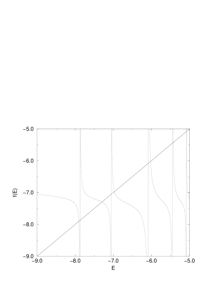
Figure 4: $f(E)$ versus E for $10\times 11$ lattice with ${\bf P}=(0,0)$ and $E_{0}=-7.365$ (i.e., $E_{0}={\cal E}(0,1)+{\cal E}(0,-1)$.) The top graph (dotted line) is for boson $f(E)=E_{0}+T_{1,1}(E)$, and the top graph (solid line) for fermion $f(E)=E_{0}+T_{1,-1}(E)$. The fermion curve is essentially flat near $E=E_{0}$.

The intersections closest to $E_{0}=-7.365$ are $-7.299$, the first excited boson energy (see Table 1), and $-7.311$, the lowest fermion energy. Note that the curve on which the fermion intersection ($-7.311$) lies is very flat. In other words for this fermion energy $E\approx E_{0}+T(E_{0})$, i.e., the first iteration using the noninteracting energy gives an energy very close to the exact value. More precisely, we find with $E_{0}=-7.365014$, $f(E_{0})=E_{0}+T(E_{0})=-7.310584$, which is very close to $E=-7.31178$. Many t-matrix calculations,Kanamori ; Mattis ; RudinMattis ; Yosida use the first iteration $E\approx E_{0}+T(E_{0})$ as an approximation to the exact energy, and we see in this case this approximation is very good. (We will come back to this point later in Sec. III.5.)

III.4.3 ${N_{0}}=4$ case

Figure 5: Boson $f(E)$ versus E for $10\times 11$ lattice with ${\bf P}=(0,0)$ and $E_{0}=-6.601$. The dotted line is for $T_{1,1,1,1}$ and the horizontal dot-dashed line for $T_{1,1,-1,-1}$ (which corresponds to a noninteracting state, see text at the end of this section).

Figure 6: Fermion $f(E)$ versus E for $10\times 11$ lattice with ${\bf P}=(0,0)$ and $E_{0}=-6.601$. The solid line is for $T_{1,-1,1,-1}$ and the long-dashed line for $T_{1,-1,-1,1}$. Note that closely spaced fermion energy pairs are separated by symmetry.

In Figs. 5 and 6, we plot $f(E)$ for $E_{0}={\cal E}(1,-1)+{\cal E}(-1,1)={\cal E}(1,1)+{\cal E}(-1,-1)=-6.601$ and ${\bf P}=(0,0)$. For this ${N_{0}}=4$ case we have two boson functions, plotted in Fig. 5, $f(E)=E_{0}+T_{1,1,1,1}(E)$ (dotted line) and $f(E)=E_{0}+T_{1,1,-1,-1}(E)$ (dot-dashed line), and we have two fermion functions, plotted in Fig. 6, $f(E)=E_{0}+T_{1,-1,1,-1}(E)$ (solid line) and $f(E)=E_{0}+T_{1,-1,-1,1}(E)$ (dashed line). The fermion intersections closest to $E_{0}$ are $-6.499$ and $-6.470$. Here again the two fermion curves are very flat. The two boson intersections closest to $E_{0}$ are $-6.022$ and $-6.601$. Note that the latter is also a noninteracting energy, and it is the intersection of the horizontal line $E=E_{0}$ with $y=E$.

One interesting observation of the fermion plot in Fig. 6 is that pairs of closely spaced energies (for example $-7.311$ and $-7.177$) lie on different symmetry curves. We know that if we have a square lattice (for example $10\times 10$) then the noninteracting fermion energies come in pairs. Here, we have chosen a $10\times 11$ lattice that is close to a square but does not have exact degeneracies. We see that the resulting closely spaced pairs are separated by symmetry considerations.

Another interesting observation from Fig. 5 for bosons is that we have a horizontal line that corresponds to $T_{1,1,-1,-1}(E)=0$. For this case the noninteracting energy is an exact energy. That is to say, $(1,1,-1,-1)$ is a null vector of ${\cal T}(E)$ (see Sec. III.3.3), or the eigenstate,

$$|{\bf q}_{1},{\bf q}_{2}\rangle+|{\bf q}_{2},{\bf q}_{1}\rangle-|{\bf q}_{3},{\bf q}_{4}\rangle-|{\bf q}_{4},{\bf q}_{3}\rangle,$$ (79)

with ${\bf q}_{3}=(q_{1x},q_{2y})$ and ${\bf q}_{4}=(q_{2x},q_{1y})$ is an exact eigenstate of the Hamiltonian. This can be shown easily using the Schrodinger equation Eq. (18). We have $g({\bf q}_{1})=g({\bf q}_{2})=1$, $g({\bf q}_{3})=g({\bf q}_{4})=-1$, and $g({\bf q})=0$ for all other ${\bf q}$, and we can easily show $V({\bf q}-{\bf q}_{1})+V({\bf q}-{\bf q}_{2})-V({\bf q}-{\bf q}_{3})-V({\bf q}-{\bf q}_{4})=0$ (because $V({\bf k})$ can be separated into a sum of two terms that involve the $x$ and $y$ components separately).

Transforming to the real space, without worrying about normalization, we can have

$${\tilde{g}}({\bf r}) = \sum_{\bf q}e^{-i{\bf q}\cdot{\bf r}}g({\bf q})$$ (80)

$$\sim \left(e^{-iq_{1x}x}-e^{-iq_{2x}x}\right)\left(e^{-iq_{1y}y}-e^{-iq_{2y}y}\right),$$

where we have used the fact mentioned above that $g({\bf q})$ is not zero for only four ${\bf q}$’s which are related by pair component exchange symmetry. It is clear from Eq. (80) that ${\tilde{g}}(0,y)=0={\tilde{g}}(x,0)$, which means that the wave function in relative position space is “d-wave” like, having nodes along $x$ and $y$ axes (thus happens to have nodes at every relative position where the potential would be nonzero).

III.5 Fermion: noninteracting to interacting

In this section we use the t-matrix techniques developed in the preceding sections of this section to study the relationship between the noninteracting energies and the interacting energies. We start with the table of energies in Table 1 for the $10\times 11$ lattice with ${\bf P}=(0,0)$. We have asked in the introduction to this section whether we can go from the noninteracting to the interacting energies and now we know that we have an equation $E=E_{0}+T(E)$ where $T(E)$ is the symmetry reduced scalar t-matrix function. From our graphs (Fig. 4 and Fig. 6) we have commented that for fermions the curve of $T(E)$ around $E_{0}$ is quite flat (which is not the case for bosons). And we mentioned that this implies that the approximation $E\approx E_{0}+T(E_{0})$ is close to the exact energy. Now in this section, we study the t-matrix approach for a specific system. We will denote $E_{1}=E_{0}+T(E_{0})$, the first iteraction result, and $E_{n+1}=E_{0}+T(E_{n})$, the $n$th iteration result.

In Table 2 we show the t-matrix calculation for the $10\times 11$ lattice. We show for the lowest few states the noninteracting energy $E_{0}$, the first t-matrix iteration $E_{1}$, the fifth t-matrix iteration $E_{5}$, and the exact energy $E_{\rm exact}$. In Fig. 7 these energy levels are plotted graphically. From the table, it is clear that the first t-matrix iteration result $E_{1}$ is quite close to the exact energy, and the fifth iteration result $E_{5}$ gives a value that is practically indistinguishable from the exact value.

Table 2: Fermion energies for $10\times 11$ lattice with ${\bf P}=(0,0)$. $E_{0}={\cal E}({\bf q}_{1})+{\cal E}({\bf q}_{2})$ is the noninteracting energy. $E_{n}=E_{0}+T(E_{n-1})$ where $T(E)$ is the symmetry reduced t-matrix. Here only fermion energies (from $T_{1,-1}$ or $T_{1,-1,1,-1}$ and $T_{1,-1,-1,1}$) are included.

${\bf q}_{1}$	${\bf q}_{2}$	$E_{0}$	$E_{1}$	$E_{5}$	$E_{\rm exact}$
(0,1)	(0,-1)	-7.365014	-7.310598893	-7.311780378	-7.311780378
(1,0)	(-1,0)	-7.236067	-7.17521279	-7.17705944	-7.177059442
(1,-1)	(-1,1)	-6.601082	-6.493807907	-6.49940706	-6.49940711
(1,1)	(-1,-1)	-6.601082	-6.460962404	-6.470087137	-6.470087302
(0,2)	(0,-2)	-5.661660	-5.532751985	-5.54494225	-5.544943745
(2,0)	(-2,0)	-5.236067	-5.134290466	-5.147558003	-5.147567483

Figure 7: Two-fermion energy levels for the $10\times 11$ lattice with ${\bf P}=(0,0)$. From left to right, the lowest few noninteracting energies $E_{0}$, first t-matrix iteration $E_{1}$, fifth t-matrix iteration $E_{5}$, and the exact energy $E_{\rm exact}$ are plotted. Note that the third noninteracting energy from the bottom is doubly degenerate (see Table 2).

IV A Few Fermions: Shell Effect and T-Matrix

In Sec. II, we used lattice Green function to study the problem of two particles (bosons and fermions), and at the end of that section, in Sec. II.4, we obtained the ground state energy of a few particles on a large lattice by summing up the energy of each pair of particles. This section contains a much more detailed study of the few-fermion problem: we will consider first the fermion shell effect and then we will study the interaction correction to energy (ground state and excited states) for a few fermions (three, four, and five) using the t-matrix.

Our results – summarized in Sec. IV.6 – confirm that, in the dilute limit, almost all of the interaction correction is accounted for by the two-body terms of the t-matrix approximation, Eq. (81). But (recall Eq. (3)) that is a hallmark of a Fermi liquid picture; i.e., our numerical results suggest its validity at low densities. This is a nontrivial result, in that firstly, the validity of Fermi liquid theory in a finite-system context has rarely been considered. Standard t-matrix theory depends on a Fermi surface which (at $T=0$) is completely sharp in momentum space, and every pair’s t-matrix excludes scattering into the same set of occupied states. In a finite system, however, the allowed ${\bf q}$ vectors fall on a discrete grid, and since the total number of particles is finite, the t-matrices of different pairs see a somewhat different set of excluded states (since they do not exclude themselves, and one particle is a non-negligible fraction of the total).

Secondly, and more essentially, the analytic justifications of Fermi liquid theory exist only in the cases of spinfull fermions (in a continuum). That case is dominated by s-wave scattering, so that the t-matrix approaches a constant in the limit of small momenta (and hence in the dilute limit). Our spinless case is rather different, as will be elaborated in Sec. V, because the t-matrix is dominated by the p-wave channel, which vanishes at small momenta. Thus the ${\bf q}$ dependence is crucial in our case, and the numerical agreement is less trivial than it would be for s-wave scattering.

In this section, after an exhibition of the shell effect (Sec. IV.1), we present a general recipe for the multi-fermion t-matrix calculation. This is developed by the simplest cases, chosen to clarify when degeneracies do or do not arise.

IV.1 Fermion shell effect

At zero temperature, the ground state of noninteracting fermions is formed by filling the one-particle states one by one from the lowest to higher energies. For our model of spinless fermions on a square lattice, we have the two ingredients for the shell effect: fermionic exclusion and degeneracies of one-particle states due to the form of our energy function and lattice symmetry. Shell effects have been noted previously in interacting models; Shell our code, permitting non-rectangular boundary conditions, allows us to see even more cases of them

In Fig. 8 we show the exact and for comparison the noninteracting ground state energies for the $5\times 8$ and $7\times 7$ lattices for up to seven particles. The energy increment curve $E(M)-E(M-1)$ is plotted and shows clearly the shell effect.

Figure 8: Shell effect for $5\times 8$ and $7\times 7$ lattices. Exact, interacting groundstate energies are compared with noninteracting energies for up to seven particles. Energy increment $E(M)-E(M-1)$ is shown.

The filled shells for the $5\times 8$ lattice are at $M=3$ (with momentum vectors $(0,0)(0,\pm 1)$ occupied) and $M=5$ (with $(0,0)(0,\pm 1)(\pm 1,0)$ occupied). On the other hand, $M=3$ is not a filled shell of the $7\times 7$ lattice. For comparison, we show the boson energy plot for the $5\times 8$ lattice in Fig. 9. Because bosons can all be at the zero-momentum state, where energy is $-4$, the total noninteracting energy is $-4M$. The exact energy curve shows smooth changes when $M$ increases. There is no shell effect.

Figure 9: Boson noninteracting and exact groundstate energies for the $5\times 8$ lattice with one to seven particles. Because bosons can all be at the zero-momentum state, where the energy is $-4$, the noninteracting energy is $-4M$. The exact energy shows smooth changes when $M$ increases. There is no shell effect.

IV.2 General multi-fermion theory

The key notion for generalizing our two-fermion approach to $M$ fermions is that the set ${Q_{0}}$ now consists of every $M$-tuple $\alpha$ of wavevectors that gives the same total momentum and noninteracting energy. This defines a reduced Hilbert space, with the corresponding basis states $|\phi_{\alpha}\rangle$. We can construct an approximate, effective Hamiltonian $H_{0}+H_{\rm tm}$ acting within ${Q_{0}}$-space, where $H_{\rm tm}$ is a sum of pairwise t-matrix terms, each of which changes just two fermion occupancies:

$$H_{\rm tm}={\sum}^{\prime}_{\alpha\beta}{\bf T}_{\alpha\beta}$$ (81)

The notation ${\sum}^{\prime}_{\alpha\beta}$ means the sum only includes the pair $(\alpha,\beta)$ when $|\phi_{\alpha}\rangle$ differs from $|\phi_{\beta}\rangle$ by a change of two fermions.

Thus, each term in Eq. (81) is associated with a particular fermion pair $({\bf q}_{i},{\bf q}_{j})$. Each such pairwise t-matrix can be viewed as a sum of all possible repeated scatterings of those two fermions through intermediate states, except that intermediate states which are already included in ${Q_{0}}$ are excluded. (The most important omission of this approximation would be the processes in which three or more fermions are permutated before the system returns to the ${Q_{0}}$ Hilbert space.) Each term is a two-fermion t-matrix calculated according to the recipe of Secs. III.2 and III.4 – thus each term has its own two-fermion wavevector set ${Q_{0}}^{i,j}$ and complementary set ${\bar{Q}}^{i,j}$, as defined in Eq. (53). The only change in the recipe is to augment the set ${\bar{Q}}^{i,j}$ of wavevectors forbidden in the intermediate scatterings of the two fermions, since they cannot scatter into states already occupied by the other fermions in states $\alpha$ and $\beta$. (See Eq. (82) for an example.)

The t-matrix treatment is a form of perturbation expansion, for which the small parameter is obviously not $V$ (which is large) but instead $1/L^{2}$, as is evident from Eq. (47). That is, as the lattice size is increased (with a fixed set of fermions), the approximation captures a larger and larger fraction of the difference $E_{\rm exact}-E_{0}$.

IV.3 A three-fermion t-matrix calculation

We first compute the energy of three fermions ($M=3$) for the $8\times 9$ lattice with ${\bf P}=0$. For this example calculation, we have chosen $L_{x}\neq L_{y}$ to reduce the number of degeneracies in the noninteracting spectrum. In Fig. 10 we show the lowest five noninteracting levels and the corresponding states in momentum space.

Figure 10: Lowest five noninteracting energy levels for the $8\times 9$ lattice with $M=3$ fermions and total momentum ${\bf P}=(0,0)$. States in momentum space are drawn.

Let us consider the lowest noninteracting state in the $8\times 9$, ${\bf P}=(0,0)$, and $M=3$ system, with three momentum vectors: ${\bf q}_{1}=(0,1)$, ${\bf q}_{2}=(0,0)$, and ${\bf q}_{3}=(0,-1)$ (see Fig. 10). And let us first consider the interaction of the pair ${\bf q}_{1}$ and ${\bf q}_{2}$. The noninteracting energy of the pair is $E^{12}_{0}={\cal E}({\bf q}_{1})+{\cal E}({\bf q}_{2})=-7.682507$ and the total momentum is ${\bf P}_{12}={\bf q}_{1}+{\bf q}_{2}=(0,1)$. As usual, we use $E^{12}_{0}$ and ${\bf P}_{12}$ to form the set ${Q_{0}}^{12}$ (Eq. (53)). Here there are no other degenerate vectors so ${Q_{0}}^{12}=\{(0,0),(0,1)\}$. The three-particle problem is different from the two-particle case in the choice of ${\bar{Q}}^{12}$, the set of momentum vectors that the two particles can scatter into. Due to the presence of the third particle and Pauli exclusion, the two particles at ${\bf q}_{1}=(0,1)$ and ${\bf q}_{2}=(0,0)$ cannot be scattered into the momentum vector ${\bf q}_{3}=(0,-1)$, so we must exclude ${\bf q}_{3}$ from ${\bar{Q}}^{12}$. Furthermore, even though there is no particle at ${\bf P}_{12}-{\bf q}_{3}=(0,1)-(0,-1)=(0,2)$, this momentum cannot be scattered into, because otherwise the other particle would be scattered into the occupied ${\bf q}_{3}$. That is to say, the momentum vectors that can be scattered into are

$${\bar{Q}}^{12}=\{{\bf q}|{\bf q}\neq{\bf q}_{1},{\bf q}_{2},{\bf q}_{3},{\bf P}_{12}-{\bf q}_{3}\}$$ (82)

This exclusion is shown graphically in Fig. 11.

The t-matrix formalism can then be applied using ${Q_{0}}^{12}$ and ${\bar{Q}}^{12}$ to compute energy correction ${\tilde{T}}^{12}(E_{12})$ for the interaction of the ${\bf q}_{1}$ and ${\bf q}_{2}$ pair. Here ${\tilde{T}}^{12}(E)$ here is the “fermion” function $T_{1,-1}(E)$ (Eq. (73)), corresponding to the antisymmetric eigenvector of the t-matrix ${\tilde{\cal T}}(E)$; the tilde denotes the modification due to exclusion of the set ${\bar{Q}}^{12}$. When the t-matrix contributes a small correction, it is accurate to use the bare values, $E^{0}_{ij}\equiv{\cal E}({\bf q}_{i})+{\cal E}({\bf q}_{j})$, and this approximation was used for all tables and figures in this section.

The total energy within this approximation is a sum of the t-matrix corrections for all possible pairs in the system, which are $({\bf q}_{2},{\bf q}_{3})$, and $({\bf q}_{1},{\bf q}_{3})$ in the present case:

$$E_{\rm tm}={\cal E}({\bf q}_{1})+{\cal E}({\bf q}_{2})+{\cal E}({\bf q}_{3})+{\tilde{T}}^{12}(E_{12})+{\tilde{T}}^{13}(E_{13})+{\tilde{T}}^{23}(E_{23}).$$ (83)

This is a special case of the effective Hamiltonian Eq. (81), which reduces to a $1\times 1$ matrix in the nondegenerate case. (That is, whenever the set ${Q_{0}}$ of multi-fermion occupations has just one member.) The momentum space exclusions due to the presence of other particles are depicted in Fig. 11, and the numerical values of this calculation are given in Table 3.

A more accurate approximation is to enforce a self-consistency,

$$E_{ij}\equiv E_{ij}^{0}+{\tilde{T}}^{ij}(E_{ij})$$ (84)

where as defined above $E_{ij}^{0}\equiv{\cal E}({\bf q}_{i})+{\cal E}({\bf q}_{j})$. It should be cautioned that the physical justification is imperfect: if we visualize this approximation via a path integral or a Feynman diagram, the self-consistent formula would mean that other pairs may be scattering simultaneously with pair $(ij)$, yet we did not take into account that the other pairs’ fluctuations would modify the set of sites ${\bar{Q}}^{ij}$ accessible to this pair. In any case, analogous to the two-particle t-matrix (Sec. III), we could solve Eq. (84) iteratively setting $E_{ij}^{n+1}=E_{ij}^{0}+{\tilde{T}}^{ij}(E_{ij}^{n})$, until successive iterates agree within a tolerance that we chose to be $10^{-15}$, which happened after some tens iterations.

Figure 11: Momentum space exclusions in t-matrix $M=3$ calculation for the state (0,0)(0,1)(0,-1). The crosses indicate exclusions when calculating pair energy for (0,0)(0,1) (left figure), (0,0)(0,-1) (middle), and (0,1)(0,-1) (right) respectively.

Table 3: T-matrix calculation for the $8\times 9$ lattice with $M=3$ noninteracting particles ${\bf q}_{1}=(0,0)$, ${\bf q}_{2}=(0,1)$, and ${\bf q}_{3}=(0,-1)$. The total noninteracting energy is $E_{0}={\cal E}({\bf q}_{1})+{\cal E}({\bf q}_{2})+{\cal E}({\bf q}_{3})$ and the total t-matrix correction is ${\tilde{T}}={\tilde{T}}^{12}+{\tilde{T}}^{13}+{\tilde{T}}^{23}$. The energy calculated using the t-matrix is then $E_{\rm tm}=E_{0}+{\tilde{T}}$ and the exact energy from diagonalization is $E_{\rm exact}$. $E^{ij}_{0}={\cal E}({\bf q}_{i})+{\cal E}({\bf q}_{j})$, is the noninteracting energy of the $(i,j)$ pair.

${Q_{0}}^{ij}$	${\bf P}_{ij}$	$E^{ij}_{0}$	${\tilde{T}}^{ij}$
(0,0)(0,1)	(0,1)	-7.532088886	0.041949215
(0,0)(0,-1)	(0,-1)	-7.532088886	0.041949215
(0,1)(0,-1)	(0,0)	-7.064177772	0.118684581
Column sum		${\tilde{T}}=0.202583012$
Noninteracting total		$E_{0}=-11.064177772$
T-matrix total		$E_{\rm tm}=-10.861594761$
Exact total		$E_{\rm exact}=-10.871031687$

Using the same procedure, we can also calculate the t-matrix energies for the nondegenerate excited states of the $M=3$ system in Fig. 10: the $(-1,0)(0,0)(1,0)$ and $(0,2)(0,0)(0,-2)$ states. The results are shown in Table 4. Fig. 12 shows graphically the noninteracting energy levels, the t-matrix energies for the three nondegenerate states, and the exact energies from diagonalization, and the arrows link the noninteracting energies $E_{0}$ with the t-matrix results $E_{\rm tm}=E_{0}+{\tilde{T}}$. The agreement between $E_{\rm tm}$ and $E_{\rm exact}$ is good.

Table 4: Lowest 15 noninteracting, exact, and t-matrix energies for $8\times 9$ lattice with $M=3$ and ${\bf P}=(0,0)$.

$E_{0}$	$E_{\rm exact}$	$E_{\rm tm}$
-11.064178	-10.871031687	-10.861594761
-10.828427	-10.608797838	-10.595561613
-9.892605	-9.672121352
-9.892605	-9.519017636
-9.892605	-9.497189108
-9.892605	-9.462304364
-9.892605	-9.398345108
-9.892605	-9.345976806
-8.694593	-8.252919763	-8.210179503
-8.239901	-8.015024904
-8.239901	-7.946278078
-8.239901	-7.809576487
-8.239901	-7.800570818
-8.239901	-7.690625772
-8.239901	-7.615399722

Figure 12: Noninteracting, t-matrix, and exact energies of the three-particle fermion system on the $8\times 9$ lattice with ${\bf P}=(0,0)$. The bracketed numbers refer to the degeneracies of the level (see Fig. 10). The arrows associate the noninteracting states with the t-matrix results. We have worked on nondegenerate noninteracting states so far.

IV.4 A five-fermion t-matrix calculation

We now consider briefly a $M=5$ calculation, again for the $8\times 9$ lattice. The noninteracting ground state is unique, with momentum vectors ${\bf q}_{1}=(0,0)$, ${\bf q}_{2}=(0,1)$, ${\bf q}_{3}=(0,-1)$, ${\bf q}_{4}=(1,0)$, and ${\bf q}_{5}=(-1,0)$. In Fig. 13 we show the excluded set ${\bar{Q}}^{2,4}$ of the t-matrix computation for the pair $({\bf q}_{2},{\bf q}_{4})$. The momentum vectors $({\bf q}_{1},{\bf q}_{3},{\bf q}_{5})$ filled with other fermions are excluded, of course; three more wavevectors are excluded since the other member of the pair would have to occupy one of ${\bf q}_{1}$, ${\bf q}_{3}$, or ${\bf q}_{5}$, due to conservation of the total momentum ${\bf P}=(1,1)$. The t-matrix results for all 10 pairs are presented in Table 5.

One might think that the pair, ${\bf q}_{2}=(0,1)$ and ${\bf q}_{4}=(1,0)$, exhibits pair-exchange symmetry with (0,0)(1,1), so that $N_{0}=4$ as in Sec. III.3.3 and Sec. III.4.3. However, since (0,0) is occupied, the (0,1)(1,0) pair cannot scatter into the (0,0)(1,1) pair: hence (0,1)(1,0) is a generic pair with $N_{0}^{2,4}=2$. In general, if a pair is ever free to scatter into a degenerate pair state with a different occupation, that must be part of a many-particle state degenerate with the original one. Thus, the complicated t-matrix pairs with $N_{0}^{ij}>2$ can arise in a many-fermion calculation only when the noninteracting many-fermion states are themselves degenerate.

Figure 13: Momentum space exclusions in t-matrix $M=5$ calculation for momentum vectors ${\bf q}_{2}=(0,1)$ and ${\bf q}_{4}=(1,0)$ (dots without crosses). These two fermions are excluded from scattering into momenta from the set ${\bar{Q}}^{2,4}$ (marked by crosses). The ground state is shown, with occupied momenta (0,0), (0,1), $(0,-1)$, (1,0), and $(-1,0)$ (solid dots).

Table 5: T-matrix calculation for the $8\times 9$ lattice with five particles (0,0), (0,1), $(0,-1)$, (1,0), and $(-1,0)$. The exclusions in ${\bar{Q}}$ for the pair (0,1)(1,0) are depicted in Fig. 13.

${Q_{0}}^{ij}$	$E^{ij}_{0}$	${\tilde{T}}^{ij}$
$(0,0)$ $(0,1)$	-7.532088886	0.045184994
$(0,0)$ $(0,-1)$	-7.532088886	0.045184994
$(0,0)$ $(1,0)$	-7.414213562	0.056898969
$(0,0)$ $(-1,0)$	-7.414213562	0.056898969
$(0,1)$ $(0,-1)$	-7.064177772	0.118684581
$(0,1)$ $(1,0)$	-6.946302449	0.081095408
$(0,1)$ $(-1,0)$	-6.946302449	0.081095408
$(0,-1)$ $(1,0)$	-6.946302449	0.081095408
$(0,-1)$ $(-1,0)$	-6.946302449	0.081095408
$(1,0)$ $(-1,0)$	-6.828427125	0.131405343
	$E_{0}=-17.892604897$	${\tilde{T}}=0.778639481$
	$E_{\rm exact}=-17.145715214$	$E_{\rm tm}=-17.113965417$

IV.5 Degenerate states

In the ground state examples considered up to now (Secs. IV.3 and IV.4), the noninteracting states were all nondegenerate. Let us now study a degenerate state in the third lowest level (six-fold degenerate) of $M=3$ fermions on the $8\times 9$ lattice : ${\bf q}_{2}=(0,1)$, ${\bf q}_{3}=(1,0)$, ${\bf q}_{4}=(-1,-1)$. (See Fig. 10, row 3.) In this state, the pair $[{\bf q}_{2}=(0,1),{\bf q}_{3}=(1,0)]$ has the same total energy and momentum as the pair $[{\bf q}_{1}=(0,0),{\bf q}_{5}=(1,1)]$, on account of the pair component exchange symmetry (see Sec. III.1); consequently $[{\bf q}_{2},{\bf q}_{3}]$ can be scattered into $[{\bf q}_{1},{\bf q}_{5}]$ contrary to the previous example in Sec. IV.4. Indeed, each of the six basis states in row 3 of Fig. 10 is connected to the next one by a two-body component exchange symmetry.

Following the two-fermion calculation with ${N_{0}}=4$ pairs (see Sec. III.3.3), the degenerate pairs ${\bf q}_{2}{\bf q}_{3}$ and $[{\bf q}_{1},{\bf q}_{5}]$ must be handled in the same set ${Q_{0}}^{23}$. The results Eqs. (III.3.3), (75), and (78) imply

$${\bf T}^{2,3}(E_{23})|{\bf q}_{2}{\bf q}_{3}\rangle = \frac{1}{2}(T_{1,-1,1,-1}+T_{1,-1,-1,1})|{\bf q}_{2}{\bf q}_{3}\rangle$$

$$+\frac{1}{2} ( T_{1,-1,1,-1}-T_{1,-1,-1,1})|{\bf q}_{1}{\bf q}_{5}\rangle.$$ (85)

Here $T_{1,-1,1,-1}$ and $T_{1,-1,-1,1}$ depend implicitly on ${\bf P}=(0,0)$, on the momenta, and on the energy $E_{2,3}$, as well as on ${\bar{Q}}^{23}$ which depends on the occupation (${\bf q}_{4}$) of the third fermion. In this notation, each ${\bf T}^{i,j}$ acting on any state produces two terms as in Eq. (85). The total t-matrix correction Hamiltonian is $\sum_{ij}{\bf T}^{i,j}$, summed over all 18 possible pairs appearing in the degenerate noninteracting states. When we apply this to each state in the third row of Fig. 10, we finally obtain a $6\times 6$ matrix mixing these states. Diagonalization of this matrix would give the correct t-matrix corrections (and eigenstates) for this “multiplet” of six states. We have not carried out such a calculation.

It is amusing to briefly consider the states in row 5 of Fig. 10, a different sixfold degenerate set. Unlike the row 3 case, these states separate into two subsets of three states, of which one subset has $\{q_{y}\}={-2,+1,+1}$ and the other subset has the opposite $q_{y}$ components. Scatterings cannot mix these subsets, so the $6\times 6$ matrix breaks up into two identical $3\times 3$ blocks. Hence the t-matrix energies from row 5 consist of three twofold degenerate levels. By comparison, the exact interacting energies derived from these noninteracting states come in three nearly degenerate pairs, such that the intra-pair splitting is much smaller than the (already small) splitting due to the t-matrix.

IV.6 Errors of the t-matrix

How good are the t-matrix results? From our example calculations on the $8\times 9$ lattice, in Tables 3, 4, and 5, we see that $E_{\rm tm}$ and $E_{\rm exact}$ are close.

In Fig. 14 we plot the noninteracting, t-matrix, and exact energies for $M=3$, ${\bf P}=(0,0)$ ground state on a series of near square lattices $L\times(L+1)$. The noninteracting ground state momentum vectors are $(0,0)(0,1)(0,-1)$ for this series of lattices. We do not plot for $L>12$, because, as can be seen in the bottom graph, the t-matrix energy $E_{\rm tm}$ approaches the exact energy $E_{\rm exact}$ rapidly. To see more clearly the error of the t-matrix result, we plot also $E_{\rm tm}-E_{\rm exact}$, which decays very fast as the size of the lattice increases – very roughly as the $L^{-6}$ power. Even at $L=6$, i.e. at a density $n\approx 0.05$, the t-matrix approximation captures 95% of the interaction energy $E_{\rm exact}-E_{0}$. These figures are based on using the bare energies in ${\tilde{T}}^{ij}(E_{ij})$ in Eq. (83). If we carried out the self-consistent calculation described in Sec. IV.3), the error $E_{\rm tm}-E_{\rm exact}$ would be smaller by a factor of roughly 2.5.

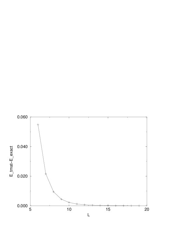
Figure 14: Noninteracting, t-matrix, and exact energies for $M=3$, ${\bf P}=(0,0)$ ground state (0,0)(0,1)$(0,-1)$ on a series of $L\times(L+1)$ lattices as a function of $L$ (top graph). $E_{\rm tm}-E_{\rm exact}$ versus $L$ (bottom graph).

V The Dilute Limit: Energy Curves

In this section, we are interested in the functional form of the energy as a function of particle density for both bosons and fermions in the dilute limit. In the three-dimensional case, the problem of dilute quantum gases with strong, repulsive, short-range interactions was first addressed in the language of diagrammatic field theory by GalitskiiGal for fermions and BeliaevBel for bosons. At that time, the ground state energy as an expansion in the particle density was also obtained for hard-sphere fermion and boson gases by Yang and collaborators HuangYang using a pseudopotential method. The field theoretical methods were later adapted to two dimensions in particular by SchickSchick for hard-disk bosons and by BloomBloom for hard-disk fermions. Some other relevant analytic papers using a t-matrix approach for the Hubbard model were discussed in Sec. I.2: KanamoriKanamori and MattisMattis in $d=3$ and Rudin and MattisRudinMattis for $d=2$.

For both hard-disk fermions and bosons in two dimensions, the leading-order correction to the noninteracting energy is found to be in the form of $n/\ln n$, where $n$ is particle density. Expansions with second-order coefficients different from the results of Schick and Bloom were found in Refs. BruchBoson, and Hines, for the boson case and in Refs. BruchFermion, and Engel2, for the fermion case. There is no consensus at this time on the correct second-order coefficient for both the boson and fermion problems.

Recently, Ref. Lieb2D, has proved rigorously the leading-order expansion of the two-dimensional dilute boson gas found by Schick.Schick Numerically, the dilute boson problem on a two-dimensional lattice has been studied using quantum Monte Carlo in Refs. Parola, and Batrouni, , and they obtain good fit with Schick’s result. As we mentioned in Sec. I.2, more recently, because of a question regarding the validity of the Fermi liquid theory in two dimensions Bloom’s calculationBloom has received renewed attention,Engel2 ; FukuHubbard but this result has not been checked by numerical studies.

V.1 Dilute bosons

For two-dimensional hard disk bosons, the energy per particle $E/M$ at the low-density limit from diagrammatic calculations is obtained (in the spirit of Ref. Bel, ) by SchickSchick

$$\frac{E}{M}=\frac{2\pi\hbar^{2}}{m}\frac{n}{|\ln(na^{2})|}\left(1+{\cal O}\left(\frac{1}{\ln(na^{2})}\right)\right),$$ (86)

where $n=M/N$ is particle density, $m$ the mass of the boson, and $a$ the two-dimensional scattering length. As mentioned above, the coefficient of the second-order term, has not been settled.

This hard-disk calculation was carried out using the kinetic energy $\hbar^{2}k^{2}/2m$. In our lattice model, our hopping energy dispersion is (Eq. (14))

$${\cal E}({\bf k})=-2t(\cos(k_{x})+\cos(k_{y}))\approx-4t+tk^{2},$$ (87)

where we have Taylor-expanded the dispersion function near ${\bf k}=0$ because in the dilute limit, at the ground state, the particles occupy momentum vectors close to zero. Therefore if we use $t=\hbar=1$ and the effective mass $m^{*}$ such that we have the form $\hbar^{2}k^{2}/2m^{*}$, then $m^{*}=1/2$ for our system. So for our model, Schick’s expansion Eq. (86) should become,

$$\frac{E}{M}=-4+\frac{4\pi n}{|\ln(n{a^{*}}^{2})|}\left(1+{\cal O}\left(\frac{1}{\ln(n{a^{*}}^{2})}\right)\right),$$ (88)

where we have used ${a^{*}}$ to denote the scattering length in our lattice system. There is no straightforward correspondence between Schick’s scattering length $a$ in the continuum and our ${a^{*}}$ on the lattice. With infinite nearest-neighbor repulsion, the closest distance that our particles can come to is $\sqrt{2}$. We expect roughly $1<{a^{*}}<\sqrt{2}$, and will determine a more precise value from curve fitting.

In Fig. 15 we show the boson energy per particle ($E/M$) versus particle per site ($M/N$) curve for ten lattices, ranging from 25 sites to 42 sites, with three or more particles ($M\geq 3$). The data from all these lattices collapse onto one curve, especially in the low-density limit.

Figure 15: Boson energy per particle $E/M$ versus particle density $M/N$ data for ten lattices and $M\geq 3$. Data from different lattices collapse onto one curve. The solid line corresponds to the fitting function $-4+4\pi n(A+B/|\ln(n{a^{*}}^{2})|)$ with ${a^{*}}=1.36$, $A=-0.016$, and $B=0.959$, which is Eq. (89) with parameters from Table 6.

Eq. (88), Schick’s result applied to our model, suggests the following leading order fitting form for $E/M$ versus $n$ at the low-density limit,

$$\frac{E/M+4}{4\pi n}=A+\frac{B}{|\ln(n{a^{*}}^{2})|}.$$ (89)

That is to say, if we plot $(E/M+4)/(4\pi n)$ versus $1/|\ln(n{a^{*}}^{2})|$, then, if Schick is correct, we should get a straight line, with intercept $A=0$ and slope $B=1$, with one adjustable parameter ${a^{*}}$.

In Fig. 16, we plot $(E/M+4)/(4\pi n)$ versus $1/|\ln(n{a^{*}}^{2})|$ for the low-density limit ($n\leq 0.15$) for three choices of ${a^{*}}=1.0,1.36,\sqrt{2}$. The data points appear to lie on straight lines.

Figure 16: $(E/M+4)/(4\pi n)$ versus $1/|\ln(n{a^{*}}^{2})|$ plot to check Schick’s formula for two-dimensional dilute bosons (Eq. (88)). The data points are for $M\geq 3$ and $n\leq 0.15$ from those in Fig. 15, for lattices from $5\times 5$ to $6\times 7$. For the three ${a^{*}}$ values, the ${a^{*}}=1.36$ choice gives $A=-0.016\approx 0$ and $B=0.959\approx 1$.

For ${a^{*}}=1.36$ the fitted intercept is $A=-0.016$ and the slope $B=0.959$. In Table 6 we show the fitted slope and intercept for a number of ${a^{*}}$ choices. The slope is zero close to ${a^{*}}=1.34$ and the intercept is zero close to ${a^{*}}=1.39$. Our data thus suggest ${a^{*}}=1.36\pm 0.03$.

Table 6: Intercept $A$ and slope $B$ in linear fitting $(E/M+4)/(4\pi n)$ versus $1/|\ln(n{a^{*}})|$ for bosons, using Eq. (89). The slope is one close to ${a^{*}}=1.33$ and the intercept is zero close to ${a^{*}}=1.39$. So we get ${a^{*}}=1.36\pm 0.03$. The fitting for three choices of ${a^{*}}$ is plotted in Fig. 16.

${a^{*}}$	$B$	$A$	${a^{*}}$	$B$	$A$	${a^{*}}$	$B$	$A$
1.00	1.855	-0.251	1.32	1.033	-0.039	1.37	0.941	-0.0099
1.10	1.547	-0.178	1.33	1.014	-0.033	1.38	0.923	-0.0043
1.20	1.289	-0.112	1.34	0.995	-0.027	1.39	0.906	0.0013
1.30	1.072	-0.050	1.35	0.977	-0.021	1.40	0.889	0.0069
1.31	1.053	-0.044	1.36	0.959	-0.016	1.414	0.865	0.015

In Fig. 15, the solid line is the function $-4+4\pi n(A+B/|\ln(n{a^{*}}^{2})|)$ using ${a^{*}}=1.36$, $A=-0.016$, and $B=0.959$, and we obtain a good fit up to $n=0.15$.

For bosons, quantum Monte Carlo can be used to obtain zero temperature energies for reasonably large systems. For a dilute boson gas on a square lattice with on-site hardcore but not nearest-neighbor interaction, Ref. Parola, has fitted the first term of Schick’s formula Eq. (86), and Ref. Batrouni, has used higher-order terms and included the fitting of the chemical potential also. The agreement is good in both studies.

V.2 Dilute fermions

For fermions, it customary to write the energy per particle expansion in terms of the Fermi wavevector $k_{F}$. For two-dimensional dilute hard disk fermions with a general spin $s$, the energy per particle from diagrammatic calculations, is obtained by BloomBloom

$$\frac{E}{M}=\frac{\hbar^{2}k_{F}^{2}}{4m}\left(1+2s\frac{1}{|\ln(k_{F}a)|}+{\cal O}\left(\frac{1}{\ln(k_{F}a)}\right)^{2}\right),$$ (90)

(see Ref. Bloom, for the spin-1/2 calculation and Ref. BruchFermion, for general $s$).

Eq. (90) means that for our spinless fermions ($s=0$), the leading order correction to the noninteracting energy in Eq. (90) is zero, which is due to the fact that Eq. (90) is derived for s-wave scattering. In our model, without spin, only antisymmetric spatial wavefunctions are allowed for fermions, and therefore the leading-order correction to the noninteracting energy should be from p-wave scattering. Ref. Fetter, contains a formula for p-wave scattering in three dimensions where the leading-order correction to $E-E_{0}$ is proportional to $(k_{F}a)^{3}$ while the s-wave correction is proportional to $k_{F}a$. We are not aware of a two-dimensional p-wave calculation in the literature,FN-Bruch and we have not worked out this p-wave problem in two dimensions. We expect that the p-wave contribution to energy should be considerably smaller than that from the s-wave term. In Sec. II.4, we have considered the case of a few fermions on a large $L\times L$ lattice, and in Fig. 1 we have studied the interaction correction to the noninteracting energy $\Delta E$. It was shown there that $\Delta E$ for our spinless fermions is much smaller than that for bosons.

Using $k_{F}^{2}=4\pi n/(2s+1)$, we can rewrite Eq. (90) as

$$\frac{E}{M}=\frac{\pi\hbar^{2}n}{(2s+1)m}\left(1+4s\frac{1}{|\ln(na^{2})|}+{\cal O}\left(\frac{1}{\ln(na^{2})}\right)^{2}\right),$$ (91)

In this form, it is revealed that the second term of Eq. (91) is identical to the first term of the boson expression Eq. (86), apart from the replacement $n\to 2sn/(2s+1)$. In other words, the dominant interaction term for spinfull fermions is identical to the ferm for bosons, provided we replace $n$ by the density of all spin species but one, i.e. of the spin species which can s-wave scatter off a given test particle.

VI Conclusion

We have studied a two-dimensional model of strongly-interacting fermions and bosons. This model is the simplest model of correlated electrons. It is very difficult to study two-dimensional quantum models with short-range kinetic and potential terms and strong interaction. There are very few reliable analytical methods, and many numerical methods are not satisfactory. With our simplified model of spinless fermions and infinite nearest-neighbor repulsion, we can use exact diagonalization to study systems much larger (in lattice size) than that can be done with the Hubbard model. One of our goals is to publicize this model in the strongly-correlated electron community.

In this paper, we made a systematic study of the dilute limit of our model, using a number of analytical techniques that so far have been scattered in the literature. We studied the two-particle problem using lattice Green functions, and we demonstrated the use the lattice symmetry and Green function recursion relations to simplify the complications brought by nearest-neighbor interactions. We derived in detail the two-particle t-matrix for both bosons and fermions, and we showed the difference between the boson and fermion cases and that for fermions the first t-matrix iteration is often a good approximation. We applied the two-fermion t-matrix to the problem of a few fermions, with modifications due to Pauli exclusion, and showed that the t-matrix approximation is good for even small lattices.

It is somewhat puzzling that with the essential role the t-matrix plays in almost every calculation in the dilute limit with strong interactions, no systematic study of the t-matrix for a lattice model has been made, as far as we know. We believe that our work on the two-particle t-matrix and the few-fermion t-matrix is first such study. Some approximations that are routinely made in t-matrix calculations are graphically presented, especially the use of first t-matrix iteration in calculating fermion energy. And we demonstrate the qualitative difference between the boson and fermion t-matrices. We believe that this study is a solid step in understanding dilute fermions in two dimensions, and is of close relevance to the 2D Fermi liquid question.

The dilute boson and fermion energy per particle curves were studied in Sec. V. The boson curve was fitted nicely with a previous diagrammatic calculation, and our work on dilute bosons complements quantum Monte Carlo results.Batrouni For the fermion problem in our model, the leading order contribution to energy is from p-wave scattering; therefore, the series of results based on s-wave calculations by Bloom,Bloom Bruch,BruchFermion and Engelbrecht, et al.Engel2 are not directly available. Hopefully, the work in progress on p-wave scattering will be completed, and our diagonalization data can shed light to the interesting problem of two dimensional dilute fermions.

Our model of spinless fermions and hardcore bosons with infinite nearest-neighbor repulsion involves a significant reduction of the size of the Hilbert space as compared to the Hubbard model. This enables us to obtain exact diagonalization results for much larger lattices than that can be done with the Hubbard model, and this also enables us to check the various analytical results (Green function, t-matrix, diagrammatics) in the dilute limit with diagonalization for much larger systems than that has been done in previous works. This paper and a companion paperstripepaper on the dense limit are the first systematic study of the spinless fermion model in two dimensions. We hope that the comprehensiveness of this paper can not only draw more attention to this so far basically overlooked model but also serve as a guide for diagonalization and analytical studies in the dilute limit.

Appendix A Exact Diagonalization Program

This section describes briefly our exact diagonalization program. It is indebted to Refs. Leung, and Lin, , which are guides for coding exact diagonalization in one dimension. Here we only describe the necessary considerations in more then one dimension, and focuses on the use translation symmetry to reduce the problem.

Our underlying lattice is the square lattice, and we take the lattice constant to be unity. The periodic boundary conditions are specified by two lattice vectors ${\bf R}_{1}$ and ${\bf R}_{2}$, such that for any lattice vector ${\bf r}$ we have ${\bf r}+n_{1}{\bf R}_{1}+n_{2}{\bf R}_{2}\equiv{\bf r}$, where $n_{1}$ and $n_{2}$ are two integers. In Fig. 17, we show two systems. The first one has ${\bf R}_{1}=(4,0)$ and ${\bf R}_{2}=(0,5)$ so the number of lattice sites is $N=20$. The second one has ${\bf R}_{1}=(4,1)$ and ${\bf R}_{2}=(1,5)$ so $N=|{\bf R}_{1}\times{\bf R}_{2}|=19$. From this example we see immediately the advantage of having skewed boundary conditions: we can have reasonably shaped systems with number of sites (here 19) not possible for an usual rectangular system.

Figure 17: Square lattices with periodic boundary conditions: $(4,0)\times(0,5)$ on the left and $(4,1)\times(1,5)$ on the right. Site numbers are shown, following the numbering convention, upward and rightward.

A site order is needed to keep track of the order of the fermion sign. The convention that we use is starting the zeroth site from the lower left corner and move progressive upward and rightward following the square lattice structure until we encounter boundaries of the lattice defined by the periodic boundary condition vectors ${\bf R}_{1}$ and ${\bf R}_{2}$ (see Fig. 17). A basis state with $M$ particles is then represented by an array of the $M$ occupied site numbers, with nearest neighbors excluded (because $V=+\infty$ in our Hamiltonian Eq. (1)). Denote such a basis state $|n\rangle$ and we have

$$H|n\rangle=-t\sum_{m\in{\cal M}}s_{m}|m\rangle,$$ (92)

where ${\cal M}$ denotes the set of states created by hopping one particle in $|n\rangle$ to an allowed nearest-neighbor site and for bosons $s_{m}=1$ always and for fermions $s_{m}=\pm 1$.FN-sm And the matrix element is $\langle m|H|n\rangle=-s_{m}t$ if $m\in{\cal M}$ and 0, otherwise.

In order to calculate for large systems, it is necessary to use symmetry to block diagonalize the Hamiltonian matrix. In our code, we use lattice translation symmetry because it works for arbitrary periodic boundaries. The eigenstate that we use is the Bloch stateLeung

$$|n{\bf k}\rangle=\frac{1}{N_{n{\bf k}}}\sum_{l=0}^{N-1}e^{-i{\bf k}\cdot{\bf R}_{l}}T_{l}|n\rangle.$$ (93)

In this expression ${\bf k}$ is a wavevector (one of $N$, where $N$ is the number of sites), ${\bf R}_{l}$ is a lattice vector $T_{l}$ is a short hand notation for translation by ${\bf R}_{l}$, and $N_{n{\bf k}}$ is a normalization factor. The original basis states are divided by translation into classes and any two states in the same class give the same Bloch state with an overall phase factor. What we need to do is to choose a representative from each class, and use this state consistently to build Bloch states. For a state $|n\rangle$ we denote its representative $|\bar{n}\rangle$.

To compute the Hamiltonian matrix elements using the Bloch states Eq. (93), let us start from a representative state $|\bar{n}\rangle$. We have, as in Eq. (92), $H|\bar{n}\rangle=-t\sum_{m\in{\cal M}}s_{m}|m\rangle$, then $H|T_{l}\bar{n}\rangle=T_{l}H|\bar{n}\rangle=-\sum_{m}s_{m}T_{l}|m\rangle$, where we have used the fact that $T_{l}$ commutes with the Hamiltonian. We have,

$$H|\bar{n}{\bf k}\rangle=\frac{1}{N_{\bar{n}{\bf k}}}\sum_{l=0}^{N-1}e^{-i{\bf k}\cdot{\bf R}_{l}}HT_{l}|\bar{n}\rangle$$

$$=-\frac{1}{N_{\bar{n}{\bf k}}}\sum_{m\in{\cal M}}s_{m}\sum_{l=0}^{N-1}e^{-i{\bf k}\cdot{\bf R}_{l}}T_{l}|m\rangle$$

$$=-\frac{1}{N_{\bar{n}{\bf k}}}\sum_{m\in{\cal M}}N_{m{\bf k}}s_{m}|m{\bf k}\rangle.$$ (94)

Next because we are interested in matrix elements between representative states, we want to connect $|m{\bf k}\rangle$ in the preceding equation to $|\bar{m}{\bf k}\rangle$. If $T_{j(m)}|\bar{m}\rangle=\sigma_{j(m)}|m\rangle$, then $|m{\bf k}\rangle=\sigma_{j(m)}e^{i{\bf k}\cdot{\bf R}_{j(m)}}|\bar{m}{\bf k}\rangle$. So we have

$$H|\bar{n}{\bf k}\rangle=-\frac{1}{N_{\bar{n}{\bf k}}}\sum_{m\in{\cal M}}N_{\bar{m}{\bf k}}s_{m}\sigma_{j(m)}e^{i{\bf k}\cdot{\bf R}_{j(m)}}|\bar{m}{\bf k}\rangle.$$ (95)

We should note that for all $m\in{\cal M}$ there can be more than one element having the same representative $|\bar{m}\rangle$. That is to say in the sum in Eq. (95), there can be more than one term with $|\bar{m}{\bf k}\rangle$. We write a new set ${\cal M}^{\prime}=\{m|m\in{\cal M}\mbox{ and $m$ has rep }\bar{m}\}$. Then we can write our matrix element equation as follows,

$$\langle\bar{m}{\bf k}|H|\bar{n}{\bf k}\rangle=-\frac{N_{\bar{m}{\bf k}}}{N_{\bar{n}{\bf k}}}\sum_{m\in{\cal M}^{\prime}}\sigma_{j(m)}e^{i{\bf k}\cdot{\bf R}_{j(m)}}s_{m}.$$ (96)

Eq. (96) is the centerpiece of the Bloch state calculation. It includes many of the complications that come with the Bloch basis set. (See Ref. Leung, for the corresponding equation in one dimension.)

Let us use ${\cal N}$ to denote the number of Bloch basis states for one ${\bf k}$. ${\cal N}$ is the dimensionality of the matrix that we need to diagonalize. For ${\cal N}$ in the order of thousands, full diagonalization (with storage of the matrix) is done using LAPACK,LAPACK and a $3156\times 3156$ matrix ($7\times 7$ with $M=18$) takes about 27 minutes.FN-machine For larger ${\cal N}$, the Lanczos method is implemented following the instructions in Ref. Leung, , We have two options. First, we store information about the matrix (i.e., for each column, a set of ($p$, $j(m)$, $\sigma_{j(m)}$) described above that contains information about the nonzero entries of the Hamiltonian matrix in this column). The $M=9$ case on $7\times 7$ lattice with ${\cal N}=1,120,744$ and tolerance $10^{-15}$ takes about 45 minutes (32 Lanczos iterations) and uses about 1.5 GB of memory. This basically reaches our memory limit.

On the other hand, we can also do Lanczos without storing matrix information. The same $M=9$ case on $7\times 7$ uses only 200 MB of memory but takes more than four hours (263 minutes), for a larger tolerance $10^{-7}$ (therefore fewer Lanczos iterations, 14). Without storing matrix information, we can calculate for larger matrices: the $M=11$ case on $7\times 7$, with ${\cal N}=1,906,532$ (the largest for the $7\times 7$ system) and tolerance $10^{-7}$, is done in 10 hours, using less than 400 MB of memory. The largest matrix we computed for this work is ${\cal N}=2,472,147$, i.e., about 2.5 million Bloch states, for $M=4$ on $20\times 20$. This takes 10 hours and uses about 550 MB of memory, for a tolerance of $10^{-7}$.

In addition, we have also installed ARPACKARPACK that uses the closely related so-called Arnoldi methods and can obtain excited state eigenvalues and eigenvectors as well. If we only need information about the ground state, our Lanczos program is considerably faster than ARPACK.

The $7\times 7$ lattice, with maximum ${\cal N}$ around 2 million, is basically the largest lattice for which we can calculate eigenenergies at all fillings. The exponential growth is very rapid after this. The $8\times 8$ lattice with 8 particles has $9,151,226$ Bloch states, and with one more particle, $M=9$, there are $30,658,325$, i.e., more than 30 million states.

Appendix B Physical meaning of ${\cal T}(E)$

In this section we give yet another derivation of the t-matrix which makes more explicit the physical meaning of $T(E,{\bf P};{\bf q},{\bf q}^{\prime})$ Eq. (65).

Before we get into a lot of algebra, let us describe the physical idea. In scattering theory we know that the Born series is a perturbation series of the scattering amplitude in terms of the potential. In Fig. 18 we show the first three terms graphically, where the first term, the first Born approximation, is particularly simple–it is the Fourier transform of the potential. We also know that when the potential is weak the first few terms are an good approximation to the scattering amplitude, but when the potential is strong, we need all terms. In this section, we will show that our t-matrix $T(E,{\bf P},{\bf q},{\bf q}^{\prime})$ is the sum of all such two-body scattering terms.

Figure 18: The three figures represent perturbative terms involving $V({\bf q}-{\bf q}^{\prime})$, $T_{2}(E,{\bf P};{\bf q},{\bf q}^{\prime})$ and $T_{3}(E,{\bf P};{\bf q},{\bf q}^{\prime})$. The t-matrix, $T(E,{\bf P};{\bf q},{\bf q}^{\prime})$, is the sum of all these terms, i.e., it is the sum of the ladder diagrams to infinite order.

We start with Eq. (18) which we copy here for convenience,

$$(E-{\cal E}({\bf q})-{\cal E}({\bf P}-{\bf q}))g({\bf q})=\frac{1}{N}\sum_{{\bf q}^{\prime}}V({\bf q}-{\bf q}^{\prime})g({\bf q}^{\prime}).$$ (97)

For ${\bf q}\in{Q_{0}}$ we break up the sum over ${\bf q}^{\prime}$ into two terms and get,

$$(E-E_{0})g({\bf q}) = \frac{1}{N}\sum_{{\bf q}^{\prime}\in{Q_{0}}}V({\bf q}-{\bf q}^{\prime})g({\bf q}^{\prime})$$ (98)

$$+ \frac{1}{N}\sum_{{\bf q}^{\prime}\in{\bar{Q}}}V({\bf q}-{\bf q}^{\prime})g({\bf q}^{\prime}).$$

For ${\bf q}\in{\bar{Q}}$ we can rewrite Eq. (97) to get,

$$g({\bf q}^{\prime})=\frac{1}{N}\sum_{{\bf q}^{\prime\prime}}\frac{V({\bf q}^{\prime}-{\bf q}^{\prime\prime})}{E-{\cal E}({\bf q}^{\prime})-{\cal E}({\bf P}-{\bf q}^{\prime})}g({\bf q}^{\prime\prime}).$$ (99)

Plug Eq. (99) into the second sum in Eq. (98) and rearrange terms, we get,

$$(E-E_{0})g({\bf q}) = \frac{1}{N}\sum_{{\bf q}^{\prime}\in{Q_{0}}}V({\bf q}-{\bf q}^{\prime})g({\bf q}^{\prime})$$ (100)

$$+ \frac{1}{N}\sum_{{\bf q}^{\prime\prime}}T_{2}(E,{\bf P};{\bf q},{\bf q}^{\prime\prime})g({\bf q}^{\prime\prime}),$$

where we have defined,

$$T_{2}(E,{\bf P};{\bf q},{\bf q}^{\prime\prime})=\frac{1}{N}\sum_{{\bf q}^{\prime}\in{\bar{Q}}}\frac{V({\bf q}-{\bf q}^{\prime})V({\bf q}^{\prime}-{\bf q}^{\prime\prime})}{E-{\cal E}({\bf q}^{\prime})-{\cal E}({\bf P}-{\bf q}^{\prime})}$$ (101)

Now break the sum over ${\bf q}^{\prime\prime}$ in Eq. (100) into two parts, and we get

$$(E-E_{0})g({\bf q}) = \frac{1}{N}\sum_{{\bf q}^{\prime}\in{Q_{0}}}V({\bf q}-{\bf q}^{\prime})g({\bf q}^{\prime})$$ (102)

$$+ \frac{1}{N}\sum_{{\bf q}^{\prime}\in{Q_{0}}}T_{2}(E,{\bf P};{\bf q},{\bf q}^{\prime})g({\bf q}^{\prime})$$

$$+ \frac{1}{N}\sum_{{\bf q}^{\prime}\in{\bar{Q}}}T_{2}(E,{\bf P};{\bf q},{\bf q}^{\prime})g({\bf q}^{\prime}).$$

Plug Eq. (99) into the last term of Eq. (102) and we get

$$(E-E_{0})g({\bf q}) = \frac{1}{N}\sum_{{\bf q}^{\prime}\in{Q_{0}}}V({\bf q}-{\bf q}^{\prime})g({\bf q}^{\prime})$$ (103)

$$+ \frac{1}{N}\sum_{{\bf q}^{\prime}\in{Q_{0}}}T_{2}(E,{\bf P};{\bf q},{\bf q}^{\prime})g({\bf q}^{\prime})$$

$$+ \frac{1}{N}\sum_{{\bf q}^{\prime}}T_{3}(E,{\bf P};{\bf q},{\bf q}^{\prime})g({\bf q}^{\prime}),$$

where we have defined

$$T_{3}(E,{\bf P};{\bf q},{\bf q}^{\prime})=\frac{1}{N^{2}}\sum_{{\bf q}^{\prime\prime},{\bf q}^{\prime\prime\prime}\in{\bar{Q}}}\frac{V({\bf q}-{\bf q}^{\prime\prime})V({\bf q}^{\prime\prime}-{\bf q}^{\prime\prime\prime})V({\bf q}^{\prime\prime\prime}-{\bf q}^{\prime})}{(E-{\cal E}({\bf q}^{\prime\prime})-{\cal E}({\bf P}-{\bf q}^{\prime\prime}))(E-{\cal E}({\bf q}^{\prime\prime\prime})-{\cal E}({\bf P}-{\bf q}^{\prime\prime\prime}))}$$ (104)

Continue this process, we obtain

$$(E-E_{0})g({\bf q})=\frac{1}{N}\sum_{{\bf q}^{\prime}\in{Q_{0}}}(V({\bf q}-{\bf q}^{\prime})$$

$$+T_{2}(E,{\bf P};{\bf q},{\bf q}^{\prime})+T_{3}(E,{\bf P};{\bf q},{\bf q}^{\prime})+...)g({\bf q}^{\prime}).$$ (105)

What we have done here is the traditional perturbation theory using iteration. Eq. (105) is the Born series for scattering amplitude. The first term $V({\bf q}-{\bf q}^{\prime})$, the Fourier transform of the potential $V({\bf r})$, is the first Born approximation. The content of higher order terms $T_{2}$, $T_{3}$, … can be obtained from their definition. Eq. (101) says that $T_{2}$ involves two scatterings under $V$, and Eq. (104) says that $T_{3}$ involves three scatterings. Thus the Born series Eq. (105) can be graphically depicted at the ladders in Fig. 18,Holstein and it involves multiple scatterings to all orders. Note that each term in the Born series is infinite for infinite potential $V$. Next we will show that summing all the terms in the series gives the t-matrix and the potential $V$ cancels out, giving a finite value.

It is easy to check that

$$T_{2}(E,{\bf P};{\bf q},{\bf q}^{\prime})=V^{2}\sum_{ij}e^{i{\bf q}\cdot{\bf R}_{i}}e^{-i{\bf q}^{\prime}\cdot{\bf R}_{j}}{\bar{\cal G}}_{ij}(E,{\bf P}),$$ (106)

where ${\bar{\cal G}}_{ij}(E,{\bf P})$ is our good old Green function Eq. (57),

$$T_{3}(E,{\bf P};{\bf q},{\bf q}^{\prime})=V^{3}\sum_{ij}e^{i{\bf q}\cdot{\bf R}_{i}}e^{-i{\bf q}^{\prime}\cdot{\bf R}_{j}}({\bar{\cal G}}(E,{\bf P}))^{2}_{ij},$$ (107)

and

$$T_{n}(E,{\bf P};{\bf q},{\bf q}^{\prime})=V^{n}\sum_{ij}e^{i{\bf q}\cdot{\bf R}_{i}}e^{-i{\bf q}^{\prime}\cdot{\bf R}_{j}}({\bar{\cal G}}(E,{\bf P}))^{n-1}_{ij}.$$ (108)

Now plug these results into Eq. (105), we get

$$(E-E_{0})g({\bf q})=\sum_{{\bf q}^{\prime}\in{Q_{0}}}\left[\frac{1}{N}\sum_{ij}e^{i{\bf q}\cdot{\bf R}_{i}}e^{-i{\bf q}^{\prime}\cdot{\bf R}_{j}}V\left(\delta_{ij}+V{\bar{\cal G}}_{ij}+V^{2}({\bar{\cal G}}_{ij})^{2}+...\right)\right].$$ (109)

Now we come to a formal step,

$$V\left(I+V{\bar{\cal G}}+V^{2}({\bar{\cal G}})^{2}+...\right)=V(I-V{\bar{\cal G}}(E))^{-1},$$ (110)

and the interesting result is that the infinite potential $V$ cancels out, giving a finite value $-{\bar{\cal G}}(E)^{-1}$.

If we can do this formal sum, then we get from Eq (109),

$$(E-E_{0})g({\bf q})=\sum_{{\bf q}^{\prime}\in{Q_{0}}}T(E,{\bf P};{\bf q},{\bf q}^{\prime})g({\bf q}^{\prime}),$$

which is exactly our momentum space T-matrix equation Eq. (64) and $T(E,{\bf P};{\bf q},{\bf q}^{\prime})$ is exactly our t-matrix Eq. (65).

References

- (1) Present address: Dept. of Physics, George Washington University, Washington, DC 20052.
- (2) E. Dagotto, Rev. Mod. Phys. 66, 763 (1994).
- (3) E. Manousakis, Rev. Mod. Phys. 63, 1 (1991).
- (4) E. H. Lieb and D. C. Mattis, Mathematical Physics in One Dimension (Academic, New York, 1966).
- (5) S. R. White, Phys. Rev. Lett. 69, 2863 (1992); S. R. White and D. J. Scalapino, Phys. Rev. Lett. 80, 1272 (1998).
- (6) Y. Nagaoka, Phys. Rev. 147, 392 (1966).
- (7) R. J. Bursill, Phys. Rev. B 60, 1643 (1999); C. J. Bolech, S. S. Kancharla, and G. Kotliar, preprint (cond-mat/0206166).
- (8) H. Q. Lin and J. E. Gubernatis, Comp. Phys. 7, 400 (1993).
- (9) G. Fano, F. Ortolani, and A. Parola, Phys. Rev. B 46, 1048 (1992).
- (10) H. Bruus and J.-C. Angles d’Auriac, Phys. Rev. B 55, 9142 (1997).
- (11) C. N. Yang and C. P. Yang, Phys. Rev. 150, 321 and 327 (1966).
- (12) G. S. Uhrig and R. Vlaming, Phys. Rev. Lett. 71, 271 (1993), Physica B 194-196, 451 (1994), Physica B 206-207, 694 (1995), Ann. Physik 4 778 (1995).
- (13) R. Shankar Rev. Mod. Phys. 66, 129 (1994).
- (14) J. E. Gubernatis, D. J. Scalapino, R. L. Sugar, and W. D. Toussaint, Phys. Rev. B 32, 103 (1985).
- (15) D. Vollhardt, in Proceedings of the Enrico Fermi School, Course CXXI, edited by Broglia and Schrieffer (North-Holland, Amsterdam, 1994).
- (16) N. G. Zhang and C. L. Henley, unpublished (cond-mat/0206421).
- (17) Note that with spinless fermions and hardcore bosons and infinite nearest-neighbor repulsion, the filling (particle per lattice site) in our model goes from 0 to 1/2 only.
- (18) C. L. Henley and N. G. Zhang, Phys. Rev. B 63, 233107 (2001).
- (19) J.-L. Pichard, G. Benenti, G. Katomeris, F. Selva, and X. Waintal, to appear in Exotic States in Quantum Nanostructures (Kluwer, Dordrecht), ed. S. Sarkar (cond-mat/0107380). One could speculate that, if their model included our infinitely strong nearest-neighbor repulsion, the Hilbert space (identical to ours) would be substantially reduced, without very much error in the energies.
- (20) L. D. Landau and E. M. Lifshitz, Statistical Physics Vol. I (Addison, Reading, 1969) p.234.
- (21) A. L. Fetter and J. D. Walecka, Quantum Theory of Many-Particle Systems (McGraw, New York, 1971).
- (22) M. Schick, Phys. Rev. A 3, 1067 (1971).
- (23) P. Bloom, Phys. Rev. B 12, 125 (1975).
- (24) J. Kanamori, Prog. Theor. Phys. 30, 275 (1963).
- (25) K. Yosida, Theory of Magnetism (Springer, Berlin, 1998) p.191.
- (26) D. C. Mattis, The Theory of Magnetism Vol. I (Springer, Berlin, 1981) p. 252.
- (27) S. Rudin and D. C. Mattis, Phys. Lett. 110A, 273 (1985).
- (28) M. Randeria, J.-M. Duan, and L.-Y. Shieh, Phys. Rev. B 41, 327 (1990).
- (29) J. R. Engelbrecht, M. Randeria, and L. Zhang, Phys. Rev. B 45, 10135 (1992).
- (30) J. R. Engelbrecht and M. Randeria, Phys. Rev. B 45, 12419 (1992).
- (31) H. Fukuyama, O. Narikiyo and Y. Hasegawa, J. Phys. Soc. Jpn. 60, 372 (1991); 60, 2013 (1991).
- (32) G. Baym, Lectures on Quantum Mechanics, Chapter 8, Cooper Pairs (Benjamin-Cummings, Reading, 1981).
- (33) S.-J. Dong and C. N. Yang, Rev. Math. Phys. 1, 139 (1989).
- (34) F. Marsiglio and J. E. Hirsch, Physica C 171, 554 (1990).
- (35) H. Q. Lin, Phys. Rev. B 44, 4674 (1991).
- (36) A. G. Petukhov, J. Galan, and J. A. Verges, Phys. Rev. B 46, 6212 (1992).
- (37) S. Basu, R. J. Gooding, and P. W. Leung, Phys. Rev. B 63, 100506 (2001).
- (38) M. Fabrizio, A. Parola, and E. Tosatti, Phys. Rev. B 44, 1033 (1991).
- (39) A. S. Blaer, H. C. Ren, and O. Tchernyshyov, Phys. Rev. B 55, 6035 (1997).
- (40) We are slightly abusing the notation . is the potential function for all space. is the value of the potential at four points ( for example). And the Fourier transform of . We will differentiate these meanings by including explicitly the argument, or . Without argument, we then mean .
- (41) The following derivation is indebted to Ref. Blaer, which solved a similar problem.
- (42) Incidentally the interesting problem of computing the resistance between two points on a lattice resistor network turns out to be an application of the lattice Green functions. See J. Cserti, Am. J. Phys. 68, 896 (2000).
- (43) S. Katsura and S. Inawashiro, J. Math. Phys. 12, 1622 (1971).
- (44) T. Morita, J. Math. Phys. 12, 1744 (1971).
- (45) Note that, anisotropic hopping dispersion , where and , also has this pair component exchange symmetry.
- (46) N. Furukawa and M. Imada, J. Phys. Soc. Jpn. 61, 3331 (1992); M. Guerrero, G. Ortiz, and J. E. Gubernatis, Phys. Rev. B 62, 600-614 (2000).
- (47) V. Galitskii, Sov. Phys. JETP 7, 104 (1958).
- (48) S. Beliaev, Sov. Phys. JETP 7, 289 (1958).
- (49) K. Huang and C. N. Yang, Phys. Rev. 105, 767 (1957); K. Huang, C. N. Yang, and J. M. Luttinger, Phys. Rev. 105, 776 (1957); T. D. Lee and C. N. Yang, Phys. Rev. 105, 1119 (1957); T. D. Lee, K. Huang, and C. N. Yang, Phys. Rev. 106, 1135 (1957).
- (50) L. W. Bruch, Physica 93A, 95 (1978).
- (51) D. F. Hines, N. E. Frankel, and D. J. Mitchell, Phys. Lett. 68A, 12 (1978).
- (52) E. H. Lieb and J. Yngvason, J. Stat. Phys. 103, 509 (2001).
- (53) F. Becca, L. Capriotti, S. Sorella, and A. Parola, Phys. Rev. B 62, 15277 (2000).
- (54) G. Batrouni, (private communication); K. Bernardet, G. G. Batrouni, J.-L. Meunier, G. Schmid, M. Troyer, and A. Dorneich, Phys. Rev. B 65, 104519 (2002).
- (55) L. W. Bruch, Physica 94A, 586 (1978). G.S. Atwal (personal communication) has also derived Eq. (90) for general .
- (56) Ref. BruchFermion, discusses spin degeneracy, but does not contain a formula for p-wave terms.
- (57) P. W. Leung and P. E. Oppenheimer, Comp. Phys. 6, 603 (1993).
- (58) is in fact a function of and , but in our discussion in this paper, we always consider a fixed column , so we omitted the dependence in the notation .
- (59) E. Anderson et al., LAPACK User’s Guide, Third Edition (Siam, Philadelphia, 1999). Both the software package and the user guide are available at http://www.netlib.org/lapack.
- (60) The computer running times in this paper are obtained using an Intel Pentium III 700 processor.
- (61) R. B. Lehoucq et al., ARPACK User’s Guide, (Siam, Philadelphia, 1998). Both the software package and the user guide are available at http://www.caam.rice.edu/software/ARPACK.
- (62) B. R. Holstein, Topics in Advanced Quantum Mechanics (Addision, Redwood, 1992) p.74.