Quasi-Particle States with Topological Quantum Numbers in the Mixed State of $d$-wave Superconductors

Abstract

We investigate the extended quasi-particle states in the mixed state of $d$-wave superconductors on the basis of the Bogoliubov-de Gennes equation. We prove that the quasi-particle eigen-states can be classified in terms of new topological quantum numbers which are related to the topological nature of the non-trivial phases of the quasi-particles. Numerical results for the quasi-particle eigen-states reveal the crossover behavior from gapless to gapped states as the flux density $B$ increases. In the strong field region quantum oscillations appear in the excitation energy of the quasi-particles.

1 Introduction

The quasi-particles in the mixed state of $d$-wave superconductors has attracted much attention in connection with the peculiar low-energy excitations under a magnetic field in high-$T_{c}$ cuprates [1, 2, 3, 4, 5, 6, 7, 8, 9, 10, 11]. In this paper we investigate the extended quasi-particle states in extremely type-II $d$-wave superconductors on the basis of the Bogoliubov-de Gennes (BdG) equation, focusing on the topological nature of the quasi-particles. It is well-known that the order parameter has a non-trivial phase in the presence of vortices, that is, the phase $\phi({\bf r})$ is a multi-valued function satisfying the relation, $\nabla\times\nabla\phi({\bf r})=2\pi\sum_{i}^{N}\delta({\bf r-R}_{i}){\bf e}_{z}$, in the mixed state where vortices ($\parallel{\bf e}_{z}$) are located at ${\bf R}_{1},{\bf R}_{2},\cdots,{\bf R}_{N}$. Then, the BdG equation contains a multi-valued function, which makes the equation intractable. Anderson noticed that the phase $\phi({\bf r})$ in the BdG equation can be eliminated in terms of a singular phase transformation, by which the BdG equation is transformed into the one containing $\nabla\phi({\bf r})$ [7]. This is an important observation, because $\nabla\phi({\bf r})$ is a single-valued function, that is, the transformed BdG equation includes only single-valued functions. However, it turns out, as shown in this paper, that the topological character of the system is not fully incorporated into the wave functions by this transformation. One should note that a superconductor containing vortices may be considered as a multi-connected system. Then, the quasi-particles moving around vortices show the AB effect [11]. From this fact one understands that the wave functions of the quasi-particles should be path-dependent single-valued functions in the presence of vortices.

In this paper we clarify the topological character of the non-trivial phases of the wave functions satisfying the BdG equation and show that the quasi-particle eigen-states have a “hidden” quantum number which is related to the homotopy class of the classical orbits of the quasi-particles. We also develop a theoretical scheme for solving approximately the BdG equation in the field region $H_{c1}\ll H\ll H_{c2}$, correcting the incomplete treatments for the topological singularity of $\phi({\bf r})$ in previous works. Numerical solutions for the extended quasi-particle states in $d$-wave superconductors are briefly presented. It is shown that the gapless quasi-particle state changes to a gapped one with increasing the flux density. In the strong field region quantum oscillations appear in the excitation energy.

2 Formulation

Consider the BdG equation for a $d_{xy}$-wave superconductor,

$$\left[\begin{array}[]{cc}h_{0}(\textbf{r},\nabla)&\hat{\Delta}(\textbf{r},\nabla)\\ \hat{\Delta}^{\ast}(\textbf{r},\nabla)&-h_{0}^{\ast}(\textbf{r},\nabla)\end{array}\right]\left[\begin{array}[]{c}u_{\alpha}(\textbf{r})\\ v_{\alpha}(\textbf{r})\end{array}\right]=E\left[\begin{array}[]{c}u_{\alpha}(\textbf{r})\\ v_{\alpha}(\textbf{r})\end{array}\right],$$ (1)

where

$$h_{0}(\textbf{r},\nabla)=\frac{1}{2m}\bigl{(}{\bf p}-\frac{e}{c}{\bf A(r)}\bigl{)}^{2}-\varepsilon_{F},$$ (2)

and $\hat{\Delta}(\textbf{r},\nabla)$ is the gap operator defined as

$$\hat{\Delta}(\textbf{r},\nabla)=-\frac{1}{k_{F}^{2}}\bigl{\{}\partial_{x},\bigl{\{}\partial_{y},\Delta(\textbf{r})\bigr{\}}\bigr{\}}-\frac{\textrm{i}}{4}\Delta({\bf r})\bigl{\{}\partial_{x},\partial_{y}\}\phi(\textbf{r}),$$ (3)

with $\{A,B\}\equiv\frac{1}{2}(AB+BA)$ [3]. In eq.(3) $\phi(\textbf{r})$ is the phase of the gap function $\Delta({\bf r})$ and the second term is added for recovering the U(1)-symmetry [12, 13]. In this paper we investigate the extended quasi-particle states outside the vortex cores in the field region $H_{c1}\ll H\ll H_{c2}$, so that we may approximate the gap function as

$$\Delta(\textbf{r})\simeq\Delta_{0}\textrm{e}^{\textrm{i}\phi(\textbf{r})},$$ (4)

neglecting the spatial dependence of the gap amplitude. In the case where $N$ vortices ($\parallel z$-axis) are located at ${\bf R_{1},\cdots,R_{N}}$ in the $xy$ plane, the phase $\phi$ in eq.(3) is dependent on the vortex positions, i.e., $\phi(\textbf{r})=\phi(\textbf{r};{\bf R_{1},\cdots,R_{N}})$, and is a multi-valued function satisfying the relation,

$$\nabla\times\nabla\phi(\textbf{r};{\bf R_{1},\cdots,R_{N}})=2\pi\sum_{i=1}^{N}\delta({\bf r-R}_{i}){\bf e}_{z}.$$ (5)

To express the BdG equation in terms of only single-valued functions, removing the multi-valued function $\phi({\bf r})$, Anderson proposed a transformation for the wave functions $u_{\alpha}$ and $v_{\alpha}$ in eq.(1) as follows [7],

$$u_{\alpha}\rightarrow u_{\alpha},\ v_{\alpha}\rightarrow\textrm{e}^{-\textrm{i}\phi}v_{\alpha},\ \ \ \ {\rm or}\ \ \ \ u_{\alpha}\rightarrow\textrm{e}^{\textrm{i}\phi}v_{\alpha}\ v_{\alpha}\rightarrow v_{\alpha}.$$ (6)

This transformation has been utilized by several authors for studying the low energy excitations in the mixed state of $d$-wave superconductors [9, 10]. On the other hand, Franz and Tešanović pointed out that the phase can be eliminated also by the transformation, $u_{\alpha}\rightarrow\textrm{e}^{\textrm{i}\phi_{e}}u_{\alpha},v_{\alpha}\rightarrow\textrm{e}^{-\textrm{i}\phi_{h}}v_{\alpha}$, if $\phi_{e}+\phi_{h}=\phi$ [8, 14]. The phase factor $\textrm{e}^{\textrm{i}\phi}$ in eq.(1) can really be excluded from the BdG equation by these transformations, but we claim that these manipulations should not be considered as the transformations. Let us suppose that the wave functions in the $N$-vortex state, $u_{\alpha}(\textbf{r}),v_{\alpha}(\textbf{r})$, are expressed as

$$\left\{\begin{array}[]{l}u_{\alpha}(\textbf{r})=\tilde{u}_{n\mu}(\textbf{r})\textrm{e}^{\textrm{i}(\frac{1}{2}-\mu)\phi({\bf r;R_{1},\cdots,R_{N}})}\\ v_{\alpha}(\textbf{r})=\tilde{v}_{n\mu}(\textbf{r})\textrm{e}^{-\textrm{i}(\frac{1}{2}+\mu)\phi({\bf r;R_{1},\cdots,R_{N}})}\end{array},\right.$$ (7)

when the non-trivial phases in the wave functions are explicitly extracted. In eq.(7) $\mu$ is assumed to be a half and integer, namely, $\mu=\pm\frac{1}{2},\pm\frac{3}{2},\cdots$. Note that the phases in eq.(7) satisfy the Franz-Tešanović condition mentioned above ($\phi_{e}+\phi_{h}=\phi$) and eq.(7) is also reduced to the Anderson’s transformation (6) for $\mu=\pm\frac{1}{2}$ if eq.(7) is considered as the transformation, $(u_{\alpha},v_{\alpha})\rightarrow(\tilde{u}_{\alpha},\tilde{v}_{\alpha})$. Hence, it is clear that the phase factor ${\rm e}^{{\rm i}\phi}$ is eliminated in the equation for $\tilde{u}_{\alpha},\tilde{v}_{\alpha}$. The new equation for $\tilde{u}_{\alpha}$ and $\tilde{v}_{\alpha}$ contains explicitly a number $\mu$, so that the energy eigenvalues explicitly depend on $\mu$. Furthermore, it turns out from the calculations shown later that the energy eigen-states can be classified in terms of $\mu$. From these results one can interpret $\mu$ as a quantum number specifying the quasi-particle eigen-states in the $N$-vortex state. Then, a set of quantum numbers $\alpha$ in eq.(7) is expressed as $\alpha=(n,\mu)$, where $n$ denotes symbolically the other quantum numbers.

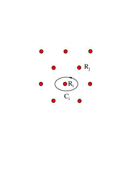
Figure 1: Closed path $C_{i}$ around the vortex located at ${\bf R}_{i}$. Solid circles denote the vortex cores.

To be convinced of our statement, let us now study the topological character of the wave functions. We introduce the operator $\mathcal{P}(C)$ which moves a function along a path $C$ [15]. Let us take a closed path $C_{i}$ around the $i$th vortex at ${\bf R}_{i}$ for $C$. Suppose that $C_{i}$ does not include any other vortices inside it (see Fig.1). Then, the operation of $\mathcal{P}(C_{i})$ on the phase $\phi({\bf r})$ induces the shift,

$$\mathcal{P}(C_{i})\phi({\bf r:R_{1},\cdots,R_{N}})=\phi({\bf r:R_{1},\cdots,R_{N}})+2\pi.$$ (8)

Suppose that the wave functions, $u_{\alpha}({\bf r})$ and $v_{\alpha}({\bf r})$, have non-trivial phases, $\Theta_{u}({\bf r})$ and $\Theta_{v}({\bf r})$, i.e., $u_{\alpha}({\bf r})=\tilde{u}_{\alpha}({\bf r})\textrm{e}^{\textrm{i}\Theta_{\alpha}^{u}({\bf r})}$ and $v_{\alpha}({\bf r})=\tilde{v}_{\alpha}({\bf r})\textrm{e}^{\textrm{i}\Theta_{\alpha}^{v}({\bf r})}$. Since $u_{\alpha}({\bf r})$ and $v_{\alpha}({\bf r})$ should be single-valued functions, we have in general

$$\mathcal{P}(C_{i})u_{\alpha}=u_{\alpha}\textrm{e}^{\textrm{i}2\pi\ell},\ \ \mathcal{P}(C_{i})v_{\alpha}=v_{\alpha}\textrm{e}^{\textrm{i}2\pi m},$$ (9)

with $\ell$ and $m$ being integers. Then, eq.(5) indicates the relations,

$$\mathcal{P}(C_{i})\Theta_{\alpha}^{u}=\Theta_{\alpha}^{u}+2\pi\ell,\ \ \ \ \mathcal{P}(C_{i})\Theta_{\alpha}^{v}=\Theta_{\alpha}^{v}+2\pi m,$$ (10)

under the conditions, $\mathcal{P}(C_{i})\tilde{u}_{\alpha}=\tilde{u}_{\alpha}$ and $\mathcal{P}(C_{i})\tilde{v}_{\alpha}=\tilde{v}_{\alpha}$. Furthermore, from the gap equation, $\Delta({\bf r})\sim\sum_{\alpha}f_{\alpha}\tilde{u}_{\alpha}\tilde{v}_{\alpha}^{\ast}\textrm{e}^{\textrm{i}(\Theta_{\alpha}^{u}-\Theta_{\alpha}^{v})}$ (see Appendix A), one may assume the equality,

$$\phi({\bf r})=\Theta_{\alpha}^{u}({\bf r})-\Theta_{\alpha}^{v}({\bf r}),$$ (11)

Then, from the operation of $\mathcal{P}(C_{i})$ on both sides of eq.(11) it follows,

$$\mathcal{P}(C_{i})\phi=\mathcal{P}(C_{i})\bigl{(}\Theta_{\alpha}^{u}-\Theta_{\alpha}^{v}\bigr{)}=\phi+2\pi(\ell-m).$$ (12)

Comparing this relation with eq.(8), one finds

$$\ell-m=1,\ \ \ \textrm{or}\ \ \ \ell=\frac{1}{2}-\mu,\ \ m=-(\frac{1}{2}+\mu),$$ (13)

with $\mu$ being a half and integer. Since these relations are simultaneously satisfied when

$$\left\{\begin{array}[]{ll}\Theta_{\alpha}^{u}({\bf r})=&(\frac{1}{2}-\mu)\phi({\bf r})\\ \Theta_{\alpha}^{v}({\bf r})=&-(\frac{1}{2}+\mu)\phi({\bf r})\end{array}\right.,$$ (14)

we obtain eq.(7). We can also show that the gap equation expressed in terms of the wave functions (7) yields $\phi({\bf r})$ for the phase of the order parameter (see Appendix A). Note that eq.(7) holds for $N=1$, i.e., the single vortex state. As is well-known, the wave functions in the 2D single vortex state are expressed as

$$\left\{\begin{array}[]{ll}u_{n\mu}(r,\theta)=\tilde{u}_{n\mu}(r)\textrm{e}^{\textrm{i}(\frac{1}{2}-\mu)\theta}\\ v_{n\mu}(r,\theta)=\tilde{v}_{n\mu}(r)\textrm{e}^{-\textrm{i}(\frac{1}{2}+\mu)\theta}\end{array}\right.,$$ (15)

where $(r,\theta)$ is the polar coordinates [16], which indicates that the phase $\phi({\bf r})$ is expressed in terms of the geometrical angle $\theta$, i.e., $\phi({\bf r})=\theta$, in this state and then $\mu$ ($=\pm\frac{1}{2},\frac{3}{2},\cdots)$ accords with the quantum number for the 2D angular momentum, though in general $\mu$ is a topological one. Thus, our conjecture (7) is consistent with the well-known result in the single vortex state. Note that $\mu$ is still a rigorous quantum number in the system with a curved vortex, in which the angular momentum is not conserved.

Let us now study the BdG equation (1), using eq.(7). In the present $d$-wave case we must be careful about the order of differentiations in eq.(3), because $\partial_{x}\partial_{y}\phi({\bf r})\not=\partial_{y}\partial_{x}\phi({\bf r})$ in the vortex state [17]. To avoid the ambiguity in the order of differentiations we symmetrize the differential operations in eq.(3) as $\partial_{x}\partial_{y}\textrm{e}^{\textit{i}\phi({\bf r})}\rightarrow\{\partial_{x},\partial_{y}\}\textrm{e}^{\textit{i}\phi({\bf r})}$. Then, substitution of eq.(7) into eq.(1) yields

$$\left[\begin{array}[]{cc}\hat{h}_{0}({\bf r},\nabla;\mu)&\Pi({\bf r},\nabla;\mu)\\ \Pi^{\ast}({\bf r},\nabla;-\mu)&-\hat{h}_{0}^{\ast}({\bf r},\nabla;-\mu)\end{array}\right]\left[\begin{array}[]{c}\tilde{u}_{n\mu}\\ \tilde{v}_{n\mu}\end{array}\right]=E\left[\begin{array}[]{c}\tilde{u}_{n\mu}\\ \tilde{v}_{n\mu}\end{array}\right],$$ (16)

where

$$\hat{h}_{0}({\bf r},\nabla;\mu)=-\frac{\hbar^{2}}{2m}\bigl{[}\nabla+\textrm{i}\frac{m}{\hbar}{\bf v}_{s}-\textrm{i}\mu\nabla\phi\bigr{]}^{2}-\varepsilon_{F},$$ (17)

${\bf v}_{s}$ is the superfluid velocity defined by

$${\bf v}_{s}=\frac{\hbar}{m}\bigl{(}\nabla\phi-\frac{2e}{\hbar c}{\bf A}\bigr{)},$$ (18)

and the off-diagonal component, $\Pi({\bf r},\nabla;\mu)$, is given as

$$\Pi({\bf r},\nabla;\mu)=-\frac{\Delta_{0}}{k_{F}^{2}}\Bigl{(}-\mu^{2}\partial_{x}\phi\cdot\partial_{y}\phi-\textrm{i}\mu\{\partial_{x},\partial_{y}\}\phi-\textrm{i}\mu\bigl{(}\partial_{y}\phi\cdot\partial_{x}+\partial_{x}\phi\cdot\partial_{y}\bigr{)}+\partial_{x}\partial_{y}\Bigr{)}.$$ (19)

To perform explicit calculations we introduce an approximation in the following. We investigate the region $H_{c1}\ll H\ll H_{c2}$ in the extremely-type II superconductors of $\kappa\gg 1$, i.e., $\xi\ll\lambda_{L}$. In this field region one can assume the relation, $\xi\ll d\ll\lambda_{L}$, where $d$ is the lattice constant of the flux-line-lattice. The spatial-dependent flux density in this region, ${\bf B}({\bf r})$, can be split into the average value, ${\bf B}_{\rm av}$, and the deviation from it, $\delta{\bf B}({\bf r})$, i.e., ${\bf B}({\bf r})={\bf B}_{\rm av}+\delta{\bf B}({\bf r})$. Since the lattice constant $d$ is much shorter than the London penetration depth $\lambda_{L}$ in this field region, the vortex currents flowing around vortices are heavily overlapped and, as a result, canceled out, which indicates the relation, $|\delta{\bf B}({\bf r})|\ll|{\bf B}_{\rm av}|$. Consequently, the spatial-dependent term $\delta{\bf B}({\bf r})$ is neglected in the 0th order approximation, ${\bf B}({\bf r})\sim{\bf B}_{\rm av}$. In this paper we confine ourselves to the lowest order approximation. Then, in this approximation we have the relation from the Maxwell equation as follows,

$$\nabla\times{\bf B}({\bf r})=\frac{4\pi e^{\ast}}{c}\rho_{s}({\bf r}){\bf v}_{s}({\bf r})\simeq\nabla\times{\bf B}_{\rm av}=0,$$ (20)

where $\rho_{s}({\bf r})$ is the local superfluid density. Since $\rho_{s}({\bf r})\simeq$ const.$\not=0$ outside the vortex cores, one can assume ${\bf v}_{s}\simeq 0$ in the present approximation. Then, noting eq.(18), we find the approximate relation,

$$\nabla\phi({\bf r})\simeq\frac{2e}{\hbar c}{\bf A}({\bf r})\simeq\frac{2e}{\hbar c}{\bf A}_{0}({\bf r}),$$ (21)

where the vector potential ${\bf A}_{0}({\bf r})$ is related to the average flux density as ${\bf B}_{\rm av}=\nabla\times{\bf A}_{0}({\bf r})$. Since ${\bf A}_{0}({\bf r})=(0,Bx,0)$ with $B=|{\bf B}_{\rm av}|$ in the Landau gauge ($B<H$), we arrive at the explicit expression for the non-trivial phase as

$$\partial_{x}\phi=0,\ \ \ \ \partial_{y}\phi=\frac{2e}{\hbar c}Bx=\frac{2\pi}{\phi_{0}}Bx,$$ (22)

where $\phi_{0}$ is the unit flux, $\phi_{0}=\frac{hc}{e^{\ast}}$. Eq.(22) indicates the relation,

$$\partial_{x}\partial_{y}\phi=\frac{2e}{\hbar c}B,\ \ \ \ \partial_{y}\partial_{x}\phi=0,$$ (23)

that is, the differential operations for $\phi$ do not commute, $\partial_{x}\partial_{y}\phi\not=\partial_{y}\partial_{x}\phi$, as expected. Then, we have the topological singularity in the present approximation,

$$(\nabla\times\nabla\phi({\bf r})|_{z}=(\partial_{x}\partial_{y}-\partial_{y}\partial_{x})\phi({\bf r})=2\pi m$$ (24)

noting $B=m\phi_{0}$ with $m$ being an integer. This result corresponds to that in the “continuity-approximation” for the singularity, i.e., $(\nabla\times\nabla\phi({\bf r}))_{z}\simeq 2\pi\langle\sum_{i}^{N}\delta({\bf r-R_{i}})\rangle_{\rm av.}=2\pi m$ [18].

Let us now solve the BdG equation, using the above approximation. Under the approximation eq.(16) can be rewritten in the 2D case as follows,

$$\left[\begin{array}[]{cc}\hat{h}_{0}(P,Q)&\Pi(P,Q;\mu)\\ \Pi^{\ast}(P,Q;-\mu)&-\hat{h}_{0}(P,Q)\end{array}\right]\left[\begin{array}[]{c}\tilde{u}_{n\mu}\\ \tilde{v}_{n\mu}\end{array}\right]=E\left[\begin{array}[]{c}\tilde{u}_{n\mu}\\ \tilde{v}_{n\mu}\end{array}\right],$$ (25)

where

$$\hat{h}_{0}(P,Q)=\mu\omega_{c}\bigl{(}Q^{2}+P^{2}\bigr{)}-\varepsilon_{F},$$ (26)

and

$$\Pi(P,Q;\mu)=\frac{\Delta_{0}}{2\varepsilon_{F}}\hbar\omega_{c}\bigl{[}\textrm{i}\mu+2\frac{\mu}{\hbar}PQ\bigr{]}.$$ (27)

Here, $\omega_{c}=\frac{eB}{mc}$ is the cyclotron frequency and

$$Q=\bigl{(}\mu\frac{2e}{c}B\bigr{)}^{-\frac{1}{2}}p_{x},\ \ \ \ P=\bigl{(}\mu\frac{2e}{c}B\bigr{)}^{-\frac{1}{2}}\bigl{(}p_{y}-\mu\frac{2e}{c}Bx\bigr{)},$$ (28)

with $p_{\alpha}=-\textrm{i}\hbar\partial_{\alpha}$. Note that $Q$ and $P$ satisfy the commutation relation, $[Q,P]=\textrm{i}\hbar$. Thus, the BdG equation is expressed in terms of only Hermitian operators and is gauge-invariant. we remark that symmetrizing the differential operations in eq.(3) is essential for obtaining the above physically-acceptable results. Now let us introduce the raising and lowering operators, $a^{\dagger}$ and $a$, as $Q=\textrm{i}\sqrt{\frac{\hbar}{2}}(a-a^{\dagger})$ and $P=\sqrt{\frac{\hbar}{2}}(a+a^{\dagger})$, noting the above commutation relation for $Q$ and $P$. Then, eq.(25) is rewritten as

$$\left[\begin{array}[]{cc}2\mu\bigl{(}a^{\dagger}a+\frac{1}{2}\bigr{)}-\varepsilon_{F}^{\prime}&-\frac{\Delta_{0}}{2\varepsilon_{F}}\mu(a^{2}-a^{\dagger 2})\\ \frac{\Delta_{0}}{2\varepsilon_{F}}\mu(a^{2}-a^{\dagger 2})&-2\mu\bigl{(}a^{\dagger}a+\frac{1}{2})+\varepsilon_{F}^{\prime}\end{array}\right]\left[\begin{array}[]{c}\tilde{u}_{n\mu}\\ \tilde{v}_{n\mu}^{\prime}\end{array}\right]=\frac{E_{n\mu}}{\hbar\omega_{c}}\left[\begin{array}[]{c}\tilde{u}_{n\mu}\\ \tilde{v}_{n\mu}^{\prime}\end{array}\right],$$ (29)

where $\tilde{v}_{n\mu}^{\prime}=-\textrm{i}\tilde{v}_{n\mu}$ and $\varepsilon_{F}^{\prime}=\frac{\varepsilon_{F}}{\hbar\omega_{c}}$. To solve eq.(29) numerically it is convenient to introduce the expansion in terms of the Landau levels,

$$\tilde{u}_{n\mu}=\sum_{k=0}^{\infty}\alpha_{2k+1}^{n\mu}|k\rangle,\ \ \ \ \tilde{v}_{n\mu}^{\prime}=\sum_{k=0}^{\infty}\alpha_{2k+2}^{n\mu}|k\rangle,$$ (30)

where $|k\rangle$ is the $k$th Landau level, i.e., $a|k\rangle=\sqrt{k}|k-1\rangle$ and $a^{\dagger}|k\rangle=\sqrt{k+1}|k+1\rangle$. It is seen that the off-diagonal components in eq.(29) induce the mixing between the Landau levels, that is, the Landau levels are not the eigen-states in the present $d$-wave case. Eq.(29) also indicates that the quasi-particle eigen-states in the mixed state of 2D $d$-wave superconductors can be classified in terms of two quantum numbers, namely $\mu$, which has the topological origin, and $n$, which is reduced to the Landau-level index in the normal state ($\Delta_{0}\rightarrow 0$). The quantum number $\mu$ is a rigorous quantum number in the mixed state of type II superconductors, which is independent of approximations used in this paper. From the above results we finally obtain the coupled equations for the coefficients, $\alpha_{k}^{n\mu}$, as

$$\frac{1}{4}\mu\tilde{\Delta}_{0}\sqrt{(k-3)(k-1)}\alpha_{k-3}^{n\mu}+[\mu k-\varepsilon_{F}^{\prime}]\alpha_{k}^{n\mu}-\frac{1}{4}\mu\tilde{\Delta}_{0}\sqrt{(k+1)(k+3)}\alpha_{k+5}^{n\mu}=\frac{E}{\hbar\omega_{c}}\alpha_{k}^{n\mu},$$ (31)

for $k=1,3,5,\cdots$, and

$$-\frac{1}{4}\mu\tilde{\Delta}_{0}\sqrt{(k-4)(k-2)}\alpha_{k-5}^{n\mu}-[\mu(k-1)-\varepsilon_{F}^{\prime}]\alpha_{k}^{n\mu}+\frac{1}{4}\mu\tilde{\Delta}_{0}\sqrt{k(k+2)}\alpha_{k+3}^{n\mu}=\frac{E}{\hbar\omega_{c}}\alpha_{k}^{n\mu},$$ (32)

for $k=2,4,6,\cdots$, with $\tilde{\Delta}_{0}=\frac{\Delta_{0}}{\varepsilon_{F}}$.

3 Numerical results and discussions

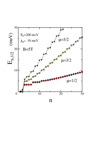
Figure 2: Energy eigen-values for the quantum numbers $\mu=\frac{1}{2},\frac{3}{2},\frac{5}{2}$ at $B=5$T in the low energy region. The eigen-value, $E_{1\mu}$, has zero-value within numerical errors.

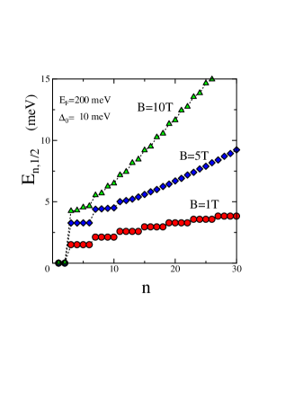
Figure 3: Energy eigen-values of $\mu=\frac{1}{2}$-band for the flux densities, $B=1,5,10$T. The relation $\hbar\omega_{c}\ll\Delta_{0}$ is satisfied in these flux densities. The zero-energy state appears in this case.

Let us now present numerical solutions of eqs.(31) and (32) obtained by a numerical diagonalization method. Fig.2 shows the positive energy eigen-values for the quantum numbers, $\mu=\frac{1}{2},\frac{3}{2},\frac{5}{2}$. The parameter values in these calculations are chosen as $\varepsilon_{F}=200$ meV, $\Delta_{0}=10$ meV, and the free electron mass $m_{e}$ is assumed in the cyclotron frequency, i.e., $\omega_{c}=\frac{eB}{m_{e}c}$. As seen in this figure, we have two quasi-particle eigen-states with nearly-zero eigen-values. These states appears in the case of $\hbar\omega_{c}\ll\Delta_{0}$ in our calculations. The existence of the zero-energy state has been predicted in the approximate calculations in ref.[7]. These zero-energy states are formed mainly by the quasi-particles lying in the nodal directions in the $k$-space. It is also seen that the two or four consecutive levels have close eigen-values in the low energy region. This result comes from that the state with index $k$ does not couple with that with $k+\ell$ of $\ell\leq 2$ or $\ell\leq 4$, as seen in eqs.(31) and (32). In Fig.3 we plot the energy eigen-values in the $\mu=\frac{1}{2}$ band for three values of $B$. Note that the relation $\hbar\omega_{c}\ll\Delta_{0}$ holds in these cases, since $\hbar\omega_{c}\sim 1.2$meV$\ll\Delta_{0}$ for $B=10$ T in the present choice of the parameter values. Then, the energy levels are essentially the same in this field region, except that the dispersion becomes steeper as $B$ increases.

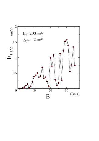
Figure 4: Dependence of the lowest excitation energy on the flux density $B$. In the weak field region, where $\hbar\omega_{c}\ll\Delta_{0}$ is satisfied, the zero-energy quasi-particle state appears. However, it changes to a gapped state above some value of $B$. In the strong field region satisfying the relation $\hbar\omega_{c}>\Delta_{0}$ the quantum oscillations appear in the quasi-particle excitation energy.

To investigate the crossover behavior due to the variation of the flux density $B$ from $\hbar\omega_{c}\ll\Delta_{0}$ to $\hbar\omega_{c}\gg\Delta_{0}$ we calculate the lowest excitation energy as a function of $B$, choosing a small value for $\Delta_{0}$. Fig.4 shows the $B$-dependence of $E_{n\mu}$ with $n=1,\mu=\frac{1}{2}$ in the case of $\Delta_{0}=2$ meV. In this choice of the parameter values we find $\hbar\omega_{c}=\Delta_{0}$ for $B\simeq 16$T. As seen in this figure, the lowest energy eigen-state has zero-energy in the weak field region of $\hbar\omega_{c}\ll\Delta_{0}$, but it abruptly changes to a gapped state above some value of $B$, which indicates that the quasi-particle eigen-states acquire a full energy-gap in the strong field region, though the symmetry of the gap function is the same as in the Meissner state. This result may be intuitively understood in the following way. The quasi-particles lying in the nodal directions with $p_{x}\sim p_{F}$ cannot turn by the effect of a weak Lorentz force when the pair-potential barrier is high. Then, in the weak filed region the quasi-particle states in the nodal directions are expected to be gapless. However, in the strong field region where the Lorentz force is strong enough, i.e., $\hbar\omega_{c}\sim\Delta_{0}$. the quasi-particles in the nodal directions can run through the pair-potential barrier. In order to excite the quasi-particles going through the barrier of the pair-potential we need a finite excitation energy, which leads to a finite energy gap. It has been proved in the GL limit, in which the Landau-level splitting is completely neglected, that the $d_{xy}$-component is induced in the mixed state of $d_{x^{2}-y^{2}}$-wave superconductors [19], which also creates fully-gapped quasi-particle states. However, the origin of the energy gap in the GL limit is completely different from that in the present theory. This result seems consistent with the experimental observation for the thermal conductivity in the mixed state [6]. In the strong field region of $\hbar\omega_{c}>\Delta_{0}$, namely $B>16$T in the present case, the lowest excitation energy shows oscillatory behavior in the $B$-dependence, as seen in Fig.4. These oscillations reflect the field dependence of the diagonal components of eq.(29), that is, they are the quantum oscillations which lead to the de Haas-van Alphen effect. Thus, our theory for the extended quasi-particles in the mixed state of $d$-wave superconductors can describes the crossover behavior from the gapless phase in the weak field region to the gapped phase showing the quantum oscillations in the strong field region.

In summary we investigated the extended quasi-particle states of $d$-wave superconductors in the field region, $H_{c1}\ll H\ll H_{c2}$, on the basis of the BdG equation. We found new topological quantum numbers which classify the quasi-particle eigen-states in the mixed state of type-II superconductors. The phase of a qausi-particle should be path-dependent in the presence of vortices, which is essentially the same as in a multi-connected system showing the Aharnnov-Bohm effect. Hence, one understands that the quantum numbers carrying information about the homotopy class of the orbit of the quasi-particle appear in the mixed state of type II superconductors. We also presented numerical solutions of the BdG equation in the field region, $H_{c1}\ll H\ll H_{c2}$. It was shown that the quasi-particle states show the crossover behavior from gappless to gapped states as the flux density increases. In the strong field region of $\hbar\omega_{c}>\Delta_{0}$ the quantum oscillations appear in the excitation energy.

Appendix A Appendix

In this Appendix we derive the gap equation in the present $d_{xy}$-superconductors. The gap function in unconventional superconductors has generally the form,

$$\Delta({\bf r,r}^{\prime})=V({\bf r-r}^{\prime})\langle\psi_{\uparrow}({\bf r})\psi_{\downarrow}({\bf r}^{\prime})\rangle$$

$$=V({\bf r-r}^{\prime})\sum_{i}\Bigl{\{}u_{i}({\bf r})v_{i}^{\ast}({\bf r}^{\prime})\bigl{[}1-f_{\rm F}(E_{i})\bigr{]}-v_{i}^{\ast}({\bf r})u_{i}({\bf r}^{\prime})f_{\rm F}(E_{i})\Bigr{\}},$$ (33)

where $V({\bf r-r}^{\prime})$ denotes the interaction between superconducting electrons. We introduce the Fourier transformation for the relative coordinates, ${\bf s}={\bf r}-{\bf r}^{\prime}$ as

$$\Delta({\bf r,r}^{\prime})=\Delta({\bf R,s})=\sum_{\bf k}\Delta({\bf R,k})\textrm{e}^{\textrm{i}{\bf k\cdot s}},\ \ \ \ \Delta({\bf R,k})=\int\textrm{d}{\bf s}\Delta({\bf R,s})\textrm{e}^{-\textrm{i}{\bf k\cdot s}},$$ (34)

with ${\bf R}=\frac{1}{2}({\bf r+r}^{\prime})$. The wave functions, $u_{i}({\bf r})$ and $v_{i}({\bf r})$, in eq.(33) are expanded in powers of the relative coordinates as

$$u_{i}({\bf R}+\frac{1}{2}{\bf s})=u_{i}({\bf R})+\frac{1}{2}({\bf s}\cdot\nabla_{\bf R})u_{i}({\bf R})+\frac{1}{8}({\bf s}\cdot\nabla_{\bf R})^{2}u_{i}({\bf R})+\cdots,$$ (35)

$$v_{i}^{\ast}({\bf R}-\frac{1}{2}{\bf s})=v_{i}^{\ast}({\bf R})-\frac{1}{2}({\bf s}\cdot\nabla_{\bf R})v_{i}^{\ast}({\bf R})+\frac{1}{8}({\bf s}\cdot\nabla_{\bf R})^{2}v_{i}^{\ast}({\bf R})+\cdots,$$ (36)

For a $d_{xy}$-wave superconductor one can utilize the following functional form for the interaction,

$$V({\bf s})=\frac{V_{d}}{k_{\rm F}^{4}}\sum_{\bf k}k_{x}^{2}k_{y}^{2}{\rm e}^{{\rm i}{\bf k\cdot s}}=\frac{V_{d}}{k_{\rm F}^{4}}\partial_{x}^{s2}\partial_{y}^{s2}\delta({\bf s}).$$ (37)

Then, substituting eqs.(35), (36) and (37) into eqs.(33) and (34), we find the Fourier component of the gap function,

$$\Delta({\bf R,k})=\frac{V_{d}}{k_{\rm F}^{4}}\sum_{i}\int{\rm d}{\bf s}\delta({\bf s})\cdot\partial_{x}^{s2}\partial_{y}^{s2}\bigl{\{}\mathcal{D}_{i}({\bf R,s})\textrm{e}^{-{\rm i}{\bf k\cdot s}}\bigl{\}}\bigl{[}1-2f_{\rm F}(E_{i})\bigr{]},$$ (38)

where

$$\mathcal{D}_{i}({\bf R,s})=\frac{1}{8}({\bf s}\cdot\nabla_{\bf R})^{2}u_{i}({\bf R})\cdot v_{i}^{\ast}({\bf R})+\frac{1}{8}u_{i}({\bf R})\cdot({\bf s}\cdot\nabla_{\bf R})^{2}v_{i}^{\ast}({\bf R})$$

$$-\frac{1}{4}({\bf s}\cdot\nabla_{\bf R})u_{i}({\bf R})\cdot({\bf s}\cdot\nabla_{\bf R})v_{i}^{\ast}({\bf R})$$ (39)

Assuming $\Delta({\bf R,k})\sim\Delta_{0}({\bf R})\hat{k}_{x}\hat{k}_{y}$ in the present $d$-wave case, we extract the $d_{xy}$-component from eq.(38) as follows,

$$\Delta({\bf R,k})=-\frac{4V_{d}}{k_{\rm F}^{2}}\sum_{i}\bigl{[}\partial_{x}^{s}\partial_{y}^{s}\mathcal{D}_{i}({\bf R,s})\bigr{]}_{{\bf s}=0}\bigl{[}1-2f_{\rm F}(E_{i})\bigr{]}\hat{k}_{x}\hat{k}_{y}.$$ (40)

Thus, the gap function is obtained as

$$\Delta_{0}({\bf R})=-\frac{4V_{d}}{k_{\rm F}^{2}}\sum_{i}\bigl{[}\partial_{x}^{s}\partial_{y}^{s}\mathcal{D}_{i}({\bf R,s})\bigr{]}_{{\bf s}=0}\tanh\frac{E_{i}}{2k_{B}T},$$ (41)

where

$$\bigl{[}\partial_{x}^{s}\partial_{y}^{s}\mathcal{D}_{i}({\bf R,s})\bigr{]}_{{\bf s}=0}=\frac{1}{4}\Bigl{\{}\partial_{x}^{R}\partial_{y}^{R}u_{i}({\bf R})\cdot v_{i}^{\ast}({\bf R})+u_{i}({\bf R})\cdot\partial_{x}^{R}\partial_{y}^{R}v_{i}^{\ast}({\bf R})$$

$$-\Bigl{[}\partial_{x}^{R}u_{i}({\bf R})\cdot\partial_{y}^{R}v_{i}^{\ast}({\bf R})+\partial_{y}^{R}u_{i}({\bf R})\cdot\partial_{x}^{R}v_{i}^{\ast}({\bf R})\Bigr{]}\Bigr{\}}.$$ (42)

Note that the above gap equation is not invariant under the U(1)-transformation,

$$\Delta_{0}({\bf r})\rightarrow\Delta_{0}({\bf r}){\rm e}^{{\rm i}\chi({\bf r})},\ \ u_{\alpha}({\bf r})\rightarrow u_{\alpha}({\bf r}){\rm e}^{\frac{1}{2}{\rm i}\chi({\bf r})},\ \ v_{\alpha}({\bf r})\rightarrow v_{\alpha}({\bf r}){\rm e}^{-\frac{1}{2}{\rm i}\chi({\bf r})}.$$ (43)

The U(1)-symmetry may be recovered by replacing the derivatives in (A.10) with “covariant” derivatives, $\partial_{\alpha}\rightarrow\partial_{\alpha}-\frac{{\rm i}}{2}\phi_{\alpha}$ where $\phi_{\alpha}\equiv\partial_{\alpha}\phi$, $\phi$ being the phase of $\Delta_{0}({\bf r})$, i.e., $\Delta_{0}({\bf r})=|\Delta_{0}({\bf r})|{\rm e}^{{\rm i}\phi({\bf r})}$ [12]. Furthermore, introducing the symmetrization for the differential operations, $\partial_{x}\partial_{y}\rightarrow\{\partial_{x},\partial_{y}\}$, we rewrite the gap equation (A.9) as follows,

$$\Delta_{0}({\bf r})=-\frac{V_{d}}{k_{\rm F}^{2}}\sum_{i}\Bigl{[}\{\partial_{x}-\frac{{\rm i}}{2}\phi_{x},\partial_{y}-\frac{{\rm i}}{2}\phi_{y}\}u_{i}({\bf r})\cdot v_{i}^{\ast}({\bf r})+u_{i}({\bf r})\cdot\{\partial_{x}-\frac{{\rm i}}{2}\phi_{x},\partial_{y}-\frac{{\rm i}}{2}\phi_{y}\}v_{i}^{\ast}({\bf r})$$

$$-(\partial_{x}-\frac{{\rm i}}{2}\phi_{x})u_{i}({\bf r})\cdot(\partial_{y}-\frac{{\rm i}}{2}\phi_{y})v_{i}^{\ast}({\bf r})-(\partial_{y}-\frac{{\rm i}}{2}\phi_{y})u_{i}({\bf r})\cdot(\partial_{x}-\frac{{\rm i}}{2}\phi_{x})v_{i}^{\ast}({\bf r})\Bigr{]}\tanh\frac{E_{i}}{2k_{B}T}.$$ (44)

Here, we change the notation, ${\bf R}\rightarrow{\bf r}$. Suppose that the wave functions, $u_{i}$ and $v_{i}$, are expressed in terms of the non-trivial phase $\phi({\bf r})$ as

$$\left\{\begin{array}[]{l}u_{n\mu}({\bf r})=\hat{u}_{n\mu}({\bf r}){\rm e}^{{\rm i}(\frac{1}{2}-\mu)\phi({\bf r})}\\ v_{n\mu}({\bf r})=\hat{v}_{n\mu}({\bf r}){\rm e}^{-{\rm i}(\frac{1}{2}+\mu)\phi({\bf r})}\end{array}\right.,$$ (45)

with $i=(n,\mu)$. The new wave functions, $\hat{u}_{n\mu}({\bf r})$ and $\hat{v}_{n\mu}({\bf r})$, are assumed to have only trivial phases. Then, substituting eq.(45) into eq.(46), we obtain the gap equation in terms of $\tilde{u}_{n\mu}$ and $\tilde{v}_{n\mu}$,

$$\Delta_{0}({\bf r})=-{\rm e}^{{\rm i}\phi({\bf r})}\cdot\frac{V_{d}}{k_{\rm F}^{2}}\sum_{n\mu}\Bigl{[}\{\partial_{x}-\frac{{\rm i\mu}}{2}\phi_{x},\partial_{y}-\frac{{\rm i\mu}}{2}\phi_{y}\}\tilde{u}_{n\mu}({\bf r})\cdot\tilde{v}_{n\mu}^{\ast}({\bf r})$$

$$+\tilde{u}_{n\mu}({\bf r})\cdot\{\partial_{x}+\frac{{\rm i\mu}}{2}\phi_{x},\partial_{y}+\frac{{\rm i\mu}}{2}\phi_{y}\}\tilde{v}_{n\mu}^{\ast}({\bf r})-(\partial_{x}-\frac{{\rm i}\mu}{2}\phi_{x})\tilde{u}_{n\mu}({\bf r})\cdot(\partial_{y}+\frac{{\rm i}\mu}{2}\phi_{y})\tilde{v}_{n\mu}^{\ast}({\bf r})$$

$$-(\partial_{y}-\frac{{\rm i}\mu}{2}\phi_{y})\tilde{u}_{n\mu}({\bf r})\cdot(\partial_{x}+\frac{{\rm i}\mu}{2}\phi_{x})\tilde{v}_{n\mu}^{\ast}({\bf r})\Bigr{]}\tanh\frac{E_{n\mu}}{2k_{B}T},$$ (46)

which indicates that the gap function $\Delta_{0}({\bf r})$ have the non-trivial phase, $\phi({\bf r})$.

References

• [1] G. E. Volovik: JETP Lett. 58, (1993) 469.
• [2] Y. Wang and A. H. Macdonald: Phys. Rev. B 52 (1995) R3876.
• [3] S. H. Simon and P. A. Lee: Phys. Rev. Lett. 78 (1997) 1548.
• [4] L. P. Gorkov and J. R. Schrieffer: Phys. Rev. Lett. 80 (1998) 3360.
• [5] K. Yasui and T. Kita: Phys. Rev. Lett. 83 (1999) 4168.
• [6] K. Krishna, N. P. Ong, Q. Li, D. Gu and N. Koshizuka: Science 277 (1997) 83.
• [7] P. W. Anderson: cond-mat/9812063.
• [8] M. Franz and Z. TeΕ‘anoviΔ‡: Phys. Rev. Lett. 84, 554 (2000); 87 (2001) 257003-1.
• [9] N. B. Kopnin and V. M. Vinokur: Phys. Rev. B 62 (2000) 9770.
• [10] J. Ye, Phys. Rev. Lett. 86 (2001) 316.
• [11] A.S. Mel’nikov: Phys. Rev. Lett. 86 (2001) 4108.
• [12] O. Vafek, A. Melikyan, M. Franz and Z. TeΕ‘anoviΔ‡: Phys. Rev. B 63 (2001) 134509.
• [13] We assume that the BdG equation (1) is invariant under a trivial phase transformation, $\phi({\bf r})\rightarrow\phi({\bf r})+\chi({\bf r})$, $u_{\alpha}({\bf r})\rightarrow u_{\alpha}({\bf r}){\rm e}^{\frac{1}{2}{\rm i}\chi({\bf r})}$, $v_{\alpha}({\bf r})\rightarrow v_{\alpha}({\bf r}){\rm e}^{-\frac{1}{2}{\rm i}\chi({\bf r})}$, with $\chi({\bf r})$ being a single-valued function.
• [14] In order to merely eliminate the phase factor in the BdG equation arbitrary functions are allowed for $\phi_{e}({\bf r})$ and $\phi_{h}({\bf r})$ as far as the condition $\phi_{e}+\phi_{h}=\phi$ is fulfilled. In the Franz-TeΕ‘anoviΔ‡ transformation the special phases are chosen for $\phi_{e}$ and $\phi_{h}$ as $\phi_{e}({\bf r})=\phi_{A}({\bf r})$ and $\phi_{h}({\bf r})=\phi_{B}({\bf r})$, where $\phi_{A}({\bf r})$ ($\phi_{B}({\bf r})$) is the non-trivial phase coming from the vortices on the A-sublattice (B-sublattice)Β [8]. The wave functions derived in ref.[8], using the Franz-TeΕ‘anoviΔ‡ transformation, does not show the correct AB effect in the $N$-vortex state. The detailed comment for the Franz-TeΕ‘anoviΔ‡ transformation will be given in a separate paper.
• [15] The operator $\mathcal{P}(C)$ which moves a function from ${\bf r}_{1}$ to ${\bf r}_{2}$ along a path $C$ is expressed as $\mathcal{P}(C)={\rm exp}\int_{0}^{1}{\rm d}\tau\frac{{\rm d}{\bf s}}{d\tau}\cdot\nabla_{\bf r}$, where the equation of path $C$ is given as $C=\bigl{\{}{\bf s}(\tau)|0\leq\tau\leq 1,{\bf s}(0)={\bf r}_{1},{\bf s}(1)={\bf r}_{2}\bigr{\}}$.
• [16] F. Gygi and M. SchlΓΌter: Phys. Rev. B 43 (1991) 7609.
• [17] This point was overlooked in previous works. In ref.[8] the terms containing $\partial_{i}\partial_{j}\phi$ are neglected on the assumption that these terms are higher-order derivatives and then they are small. In such an approximation the problem about the order of differentiations does not arise. However, the assumption is incorrect. Since $\partial_{i}\partial_{j}\phi\propto B$, as shown in our calculations, these terms should be considered as the 0th order ones in the strong field region.
• [18] The topological singularity given in eq.(5) is expanded into the Fourier series as
βˆ‡Γ—βˆ‡Ο•β€‹(𝐫)|z=2β€‹Ο€β€‹βˆ‘iNδ​(π«βˆ’π‘i)=2​π​mβ€‹βˆ‘π†ei​𝐆⋅𝐫=2​π​m+2​π​mβ€‹βˆ‘π†β‰ 0ei​𝐆⋅𝐫,evaluated-atβˆ‡βˆ‡italic-ϕ𝐫𝑧2πœ‹superscriptsubscript𝑖𝑁𝛿𝐫subscript𝐑𝑖2πœ‹π‘šsubscript𝐆superscripteβ‹…i𝐆𝐫2πœ‹π‘š2πœ‹π‘šsubscript𝐆0superscripteβ‹…i𝐆𝐫\nabla\times\nabla\phi({\bf r})|_{z}=2\pi\sum_{i}^{N}\delta({\bf r-R}_{i})=2\pi m\sum_{\bf G}{\rm e}^{{\rm i}{\bf G\cdot r}}=2\pi m+2\pi m\sum_{{\bf G}\not=0}{\rm e}^{{\rm i}{\bf G\cdot r}},
for a regular flux-line-lattice state, where ${\bf G}$ denotes the reciprocal lattice vector. In the approximation in which the terms of ${\bf G}\not=0$ are neglected one gets the approximate result given in eq.(24).
• [19] T. Koyama and M. Tachiki: Phys. Rev. B 53 (1996) 2662.
Refer to caption