From the bulk to monatomic wires: An ab-initio study of magnetism in Co systems with various dimensionality
Abstract
A systematic ab-initio study within the framework of the local-spin-density approximation including spin-orbit coupling and an orbital-polarization term is performed for the spin and orbital moments and for the X-ray magnetic circular dichroism (XMCD) spectra in hcp Co, in a Pt supported and a free standing Co monolayer, and in a Pt supported and a free standing monatomic Co wire. When including the orbital-polarization term, the orbital moments increase drastically when going to lower dimensionality, and there is an increasing asymmetry between the and XMCD signal. It is shown that spin and orbital moments can be obtained with good accuracy from the XMCD spectra via the sum rules. The term of the spin sum rule is surprisingly small for the wires, and the reason for this is discussed.
pacs:
75.30.-m, 75.90.+wThe modern methods to prepare nanostructured systems made it possible to investigate the influence of dimensionality on the magnetic properties. A central question thereby is how the qualitative behavior will change when going from two-dimensional to one-dimensional systems because it has been predicted that there is no long-range magnetic order at finite temperature in infinitely extended one-dimensional systems with short-range magnetic interactions. In the past, several experimental investigations of monolayer nanostripes of Fe on vicinal surfaces of W Elmers et al. (1994); Hauschild et al. (1998) or Cu Shen et al. (1997) have been performed, with a stripe width down to 1-10 nm. Most recently, Gambardella et al. Gambardella et al. (2000) succeeded to prepare a high density of parallel atomic chains along steps by growing Co on a high purity Pt(997) vicinal surface in a narrow temperature range. The magnetism of the Co wires was investigated Gambardella et al. (2002) by the X-ray magnetic circular dichroism (XMCD). Below a blocking temperature a long-range magnetic ordering owing to the presence of anisotropy barriers was found on the time scale of the experiment. Applying a simple model of exchange coupled superparamagnetic clusters com , the anisotropy energy could be obtained from the shape of the magnetization curve above the blocking temperature and it appeared to be much larger than the one for a Co monolayer on Pt which — in turn — is much larger than the one of hcp Co. Accordingly, a large orbital moment of per Co atom was found, the highest value ever reported for a 3d itinerant electron system.
So far, magnetism in quasi-one-dimensional systems was studied mainly in the insulating material where the magnetic Ni ions are arranged along linear chains which are well separated from each other so that the interchain interaction is only or less of the intrachain interaction. Because of the one-dimensional character of this spin system and the easy-plane anisotropy, magnetic solitons play an important role for the dynamical and thermodynamical behavior which has been investigated by neutron scattering experiments Mikeska and Steiner (1991). The discovery of magnetism in one-dimensional metallic systems opens up the chance to extend the research in many respects. First, by considering various vicinal surfaces the distance between the steps and hence the chains can be modified so that the transition from the well-isolated chains to interacting chains can be studied. Second, it is possible to grow, e.g., biatomic wires along the steps and to manipulate the wire length, and to study the respective influence on magnetic properties. Finally, we expect that the damping of magnetic excitations is larger for metals than for insulators and especially large for one-dimensional metals, possibly leading to peculiar properties of the nonlinear spin excitations Hołyst et al. (1986).
The already existing ab-initio calculations for monatomic transition metal wires considered magnetic moments Weinert and Freeman (1983); Bihlmayer et al. ; Dorantes-Dávila and Pastor (1998); Zhou et al. (1999); Spišák and Hafner (2002), exchange couplings Spišák and Hafner (2002) and magnetic anisotropies Dorantes-Dávila and Pastor (1998); Zhou et al. (1999); Eisenbach et al. (2002). It turned out Zhou et al. (1999) that in these one-dimensional systems the orbital correlations were essential and that the magnetic anisotropy and hence also the orbital moments could not be calculated reliably by the local-spin-density approximation (LSDA) in combination with spin-orbit (SO) coupling. Instead, a term correcting explicitly for the orbital correlations has to be added. It is one of the objectives of the present paper to work out the growing importance of the orbital correlations with decreasing dimensionality by calculating orbital (and spin) moments by the LSDA Perdew and Wang (1992) including SO coupling (in a self-consistent manner) without and with the orbital-polarization term Eriksson et al. (1990) which takes into account at least in part the orbital-correlation effects. The calculations are performed for Co atoms in hcp Co, in a Pt supported and in a free standing monolayer, and in a Pt supported and in a free standing monatomic wire. Another objective is to calculate the respective XMCD spectra and discuss the influence of dimensionality on the accuracy of the spin and orbital moments when these are obtained from the XMCD spectra via the sum rules Thole et al. (1992); Carra et al. (1993).
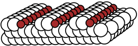
To focus on the pure effect of the dimensionality we fix the nearest-neighbor distance of the atoms for all considered systems to the one of fcc Pt (2.77Å). For the monolayers and wires we perform supercell calculations, i.e., large unit cells which model the structure are repeated periodically. In the case of the monolayer the supercell consists of two Pt and one Co {111} layers in the fcc stacking and a vacuum sheet corresponding to two empty layers. The vicinal Pt(997) surface with the Co wire at the steps is modeled by the supercell shown in Fig. 1 with two additional vacuum layers on the top.
The supercell of the free standing wire is constructed by removing all Pt atoms from this supercell. Test calculations have shown that the results change only very slightly when going to larger supercells. For the monolayers and the wires we assume perpendicular magnetization, for hcp Co it is along the c axis.
We use the tight-binding linear-muffin-tin-orbital (LMTO) method in the atomic sphere approximation Andersen and Jepsen (1984) in which we have implemented the SO coupling and the tools for calculating the XMCD spectra, and the WIEN97 code Blaha et al. (1990) which adopts the full-potential linearized-augmented-plane-wave (FLAPW) method Wimmer et al. (1981) in which the SO coupling and the tools for the calculation of the magnetooptical effects and XMCD spectra Kuneš et al. (2001a, b) and the orbital-polarization term Rodriguez et al. (2001) have been implemented. The magnetic orbital moments and spin moments are calculated directly from the wave functions as well as via the sum rules Thole et al. (1992); Carra et al. (1993) from the absorption coefficients , and for light with right-circular, left-circular and z-axis polarization at the and edge according to
| (1) | |||||
| (2) | |||||
| (3) | |||||
| (4) | |||||
| (5) |
with the XMCD signal and with . Here is the number of d holes and is the expectation value of the magnetic dipolar operator
| (6) |
where denotes the vector of the Pauli matrices. The quantities and denote the Fermi energy and a cutoff energy. For details for such type of calculations see Ref. Ederer et al., 2002. The term is negligible for cubic surroundings but it is expected to become more and more important when reducing the dimensionality of the system. Since it is very difficult to measure , this term is often neglected in the spin sum rule when analyzing the experimental data. One of the objectives of this paper is to asses this critically.
The results of the LSDA calculations with SO coupling are given in the upper part of Table 1.
| hcp | monolayer on Pt | free monolayer | wire on Pt | free wire | ||||||
| LMTO | FLAPW | LMTO | FLAPW | LMTO | FLAPW | LMTO | FLAPW | LMTO | FLAPW | |
| direct | 1.83 | 1.83 | 2.03 | 2.00 | 2.02 | 2.12 | 2.21 | 2.06 | 2.22 | 2.16 |
| d only | 1.92 | 1.87 | 2.05 | 2.02 | 2.03 | 2.12 | 2.17 | 2.02 | 2.14 | 2.11 |
| from eq. (2) | 1.79 | 1.88 | 1.96 | 2.12 | 2.03 | 2.18 | 2.09 | 2.13 | 2.14 | 2.36 |
| from eq. (2), | 1.80 | 1.86 | 1.50 | 1.77 | 1.58 | 1.62 | 1.76 | 1.94 | 2.28 | 2.26 |
| 0.001 | -0.003 | -0.066 | -0.050 | -0.064 | -0.079 | -0.048 | -0.027 | 0.021 | -0.014 | |
| direct | 0.15 | 0.15 | 0.13 | 0.13 | 0.18 | 0.19 | 0.14 | 0.14 | 0.71 | 0.40 |
| from eq. (1) | 0.15 | 0.18 | 0.12 | 0.15 | 0.17 | 0.19 | 0.14 | 0.16 | 0.70 | 0.59 |
| direct | 0.40 | 0.43 | 0.86 | 0.92 | 2.31 | |||||
| from eq (1) | 0.41 | 0.42 | 0.86 | 0.92 | 2.17 | |||||
It should be noted again that thereby we use the same nearest-neighbor distance between the atoms, i.e., the one of fcc Pt, for all structures. As explained in Ref. Ederer et al., 2002, the spin and orbital moments derived experimentally via the sum rules correspond essentially to the respective part of the valence wavefunctions with 3d angular momentum, if the “background” due to all additional contributions to the experimental absorption spectra is subtracted appropriately. We therefore compare in Table 1 the moments as calculated directly from the 3d spin and orbital densities with those obtained from the sum rules when taking into account for the absorption spectra and for the term also only that part of the valence wave functions which has 3d character. For comparison, we give also the values of directly calculated moments including all angular momentum contributions.
For all the structures there is only a slight difference between the directly calculated moments with only d contributions and with all contributions. The spin moments increase only moderately with decreasing dimensionality. For the wire on Pt our directly calculated FLAPW spin value of agrees well with the one of Ref. Bihlmayer et al., . There is also a satisfactory agreement between the directly calculated spin moments and those obtained from the spin sum rule when including the term. The contribution is negligible for hcp Co. In contrast, for the free and the Pt supported monolayers, the values of obtained from the sum rule when neglecting are between 20% and 30% smaller than the directly calculated values. Astonishingly enough, when going to even stronger reduced dimensionality, i.e., for the Pt supported wire and even more for the free wire, the term again appears to be of minor importance. To figure out the reason for this startling result, Fig. 2 shows the energy distributionWu et al. (1994) for for all the structures, i.e., the integral over the energy resolved contribution to up to an energy (for the integrals up to the Fermi level, , equals the quantity in eq. (2) ).

It becomes obvious that for the free standing monolayer and for the free standing wire, depends drastically on resulting in sharp structures in the energy distribution due to the two- or one-dimensional character of the systems. Going to the Pt supported monolayer and wire, the energy dependence of is less pronounced and the sharp structures are smeared out, indicating that these systems are not really two- or one-dimensional due to the presence of the substrate. However, obtained from the integral up to is very small for the free standing Co wire but larger for the other systems (except for hcp Co). This clearly demonstrates that the expected rule of thumb — a larger for the smaller dimensionality — does not necessarily hold. We have performed the same calculation for a free standing Ni wire. The energy distribution of is very similar but the Fermi level is shifted and is consequently much larger than for the Co wire. This again demonstrates that the symmetry arguments alone are not able to estimate the size of .
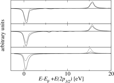
The orbital moments obtained by the LSDA calculation with SO coupling are very similar (about ) for hcp Co and for the Pt supported Co monolayer and wire, while the values are slightly larger (about ) for the free monolayer and considerably larger for the free wire. Thereby, there is a good agreement between the directly calculated orbital moments and those obtained from the calculated spectra via the sum rules. The rather small values for the Pt supported monolayer () and the Pt supported wire () are in conflict with the large corresponding experimental valuesGambardella et al. (2002) ( and ). As discussed in Ref. Zhou et al., 1999, the reason is presumably that LSDA + SO coupling does not appropriately account for orbital correlations. We therefore have redone all the calculations by including in addition the orbital-polarization term Eriksson et al. (1990). Table 1, lower part, gives the so obtained results for the orbital moments (the spin moments are nearly unaffected by this additional term). It should be noted that the calculations for hcp Co have been performed for the nearest neighbor distance of fcc Pt which explains the large moment of . For the Co monolayer on Pt (Co wire on Pt) our value () is even larger than the experimental value Gambardella et al. (2002) () which may be in part due to the fact that our calculations did not take into account any structural relaxations at the surface. For the free standing wire, the orbital moment appears to be extraordinarily high (). Obviously the experimental trend — increase of the orbital moment with decreasing dimensionality — is well reproduced when taking into account the orbital-polarization term. The increasing orbital moments result in an increasing asymmetry between the calculated and XMCD spectra (Fig. 3), in qualitative agreement with the respective experimental spectra (Fig. 2 of Ref. Gambardella et al., 2002).
Both, for the LSDA calculations with and without the orbital-polarization term, the directly calculated orbital moments agree very well with those obtained from the sum rule. Therefore, for Co in structures of various dimensionality the spin and orbital moments probably may be obtained with high accuracy from the sum rules (if including the term in the spin sum rule).
To conclude, we have shown that the orbital correlations have to be taken into account explicitly in order to reproduce the experimentally observed trend to higher orbital moments and larger asymmetries between the L3 and L2 XMCD spectra in Co systems with reduced dimensionality, and we are about to do this also for a systematic study of the magnetic anisotropy. In addition, we calculate ab initio the further parameters appearing in a model Hamiltonian for the monatomic wires, i.e., exchange interactions from the adiabatic spin wave spectra Grotheer et al. (2001), and the Gilbert damping factor Gilbert (1955). The final objective is to come to a comprehensive description of the thermodynamic properties (see Ref. com, ) and of the damped nonlinear excitations (along the lines of Ref. Hołyst et al., 1986) of monatomic magnetic linear chains.
The work at Brookhaven is supported by U.S. Department of Energy under Contract No. DE-AC02-98CH10886.
References
- Elmers et al. (1994) H. J. Elmers, J. Hauschild, H. Höche, U. Gradmann, H. Bethge, D. Heuer, and U. Köhler, Phys. Rev. Lett. 73, 898 (1994).
- Hauschild et al. (1998) J. Hauschild, H. J. Elmers, and U. Gradmann, Phys. Rev. B 57, R677 (1998).
- Shen et al. (1997) J. Shen, R. Skomski, M. Klaua, H. Jenniches, S. Sundar Manoharan, and J. Kirschner, Phys. Rev. B 56, 2340 (1997).
- Gambardella et al. (2000) P. Gambardella, M. Blanc, L. Bürgi, K. Kuhnke, and K. Kern, Surf. Sci. 449, 93 (2000).
- Gambardella et al. (2002) P. Gambardella, A. Dallmeyer, K. Maiti, M. C. Malagoli, W. Eberhardt, K. Kern, and C. Carbone, Nature 416, 301 (2002).
- (6) In this model the size of the superparamagnetic “particles” is estimated from the time-dependent kink density of the one-dimensional nearest-neighbor-exchange model in the infinite anisotropy (i.e., Ising) limit. Then these particles are considered as decoupled from each other but exposed to an external magnetic field and an anisotropy field, and the thermodynamics is described by classical Boltzmann statistics. It would be highly desirable to have a more rigorous treatment by calculating the dynamical structure factor for a one-dimensional chain with finite magnetic anisotropy and external magnetic field.
- Mikeska and Steiner (1991) H.-J. Mikeska and M. Steiner, Adv. Phys 40, 191 (1991).
- Hołyst et al. (1986) J. A. Hołyst, A. Sukiennicki, and J. J. Żebrowski, Phys. Rev B 33, 3492 (1986).
- Weinert and Freeman (1983) M. Weinert and A. J. Freeman, J. Magn. Magn. Mat. 38, 23 (1983).
- (10) G. Bihlmayer, X. Nie, and S. Blügel, unpublished data, referred to in Ref. Gambardella et al., 2002.
- Dorantes-Dávila and Pastor (1998) J. Dorantes-Dávila and G. M. Pastor, Phys. Rev. Lett. 81, 208 (1998).
- Zhou et al. (1999) L. Zhou, D. Wang, and Y. Kawazoe, Phys. Rev. B 60, 9545 (1999).
- Spišák and Hafner (2002) D. Spišák and J. Hafner, Phys. Rev. B 65, 235405 (2002).
- Eisenbach et al. (2002) M. Eisenbach, B. L. Györffy, G. M. Stocks, and B. Újfalussy, Phys. Rev. B 65, 144424 (2002).
- Perdew and Wang (1992) J. P. Perdew and Y. Wang, Phys. Rev. B 45, 13244 (1992).
- Eriksson et al. (1990) O. Eriksson, M. S. S. Brooks, and B. Johansson, Phys. Rev. B 41, 7311 (1990).
- Thole et al. (1992) B. T. Thole, P. Carra, F. Sette, and G. van der Laan, Phys. Rev. Lett. 68, 1943 (1992).
- Carra et al. (1993) P. Carra, B. T. Thole, M. Altarelli, and X. Wang, Phys. Rev. Lett. 70, 694 (1993).
- Andersen and Jepsen (1984) O. K. Andersen and O. Jepsen, Phys. Rev. Lett. 53, 2571 (1984).
- Blaha et al. (1990) P. Blaha, K. Schwarz, P. Sorantin, and S. B. Trickey, Comput. Phys. Commun. 59, 399 (1990).
- Wimmer et al. (1981) E. Wimmer, H. Krakauer, M. Weinert, and A. J. Freeman, Phys. Rev. B 24, 864 (1981).
- Kuneš et al. (2001a) J. Kuneš, P. M. Oppeneer, H.-C. Mertins, F. Schäfers, A. Gaupp, W. Gudat, and P. Novák, Phys. Rev. B 64, 174417 (2001a).
- Kuneš et al. (2001b) J. Kuneš, P. Novák, M. Diviš, and P. M. Oppeneer, Phys. Rev. B 63, 205111 (2001b).
- Rodriguez et al. (2001) C. O. Rodriguez, M. V. Ganduglia-Pirovano, E. L. Peltzer y Blancá, M. Petersen, and P. Novák, Phys. Rev. B 63, 184413 (2001).
- Ederer et al. (2002) C. Ederer, M. Komelj, M. Fähnle, and G. Schütz, Phys. Rev. B (2002), accepted for publication.
- Wu et al. (1994) R. Wu, D. Wang, and A. J. Freeman, J. Appl. Phys. 75, 5802 (1994).
- Grotheer et al. (2001) O. Grotheer, C. Ederer, and M. Fähnle, Phys. Rev. B 63, 100401 (2001).
- Gilbert (1955) T. L. Gilbert, Phys. Rev. 100, 1243 (1955).