The origin of spurious velocities in lattice Boltzmann

Abstract

Stationary droplets simulated by multi-phase lattice Boltzmann methods lead to spurious velocities around them. In this article I report the origin of these spurious velocities for one example and show how they can be avoided.

Received (August 5, 2002)Revised (revised date)

1 Introduction

Imagine a stationary droplet in quiescent conditions. For a real system there are, of course, no velocities. Yet when this simple system is simulated with a lattice Boltzmann method you will find a flow-field around the drop. Even if you start with a no flow initial condition this velocity field will develop. An example of these velocities in shown in Figure 1 (a). These velocities are know as “spurious velocities”.

The magnitude of the velocities depends on the details of the method, the radius of the drop, the surface tension and the viscosity. There have been several studies[1, 2, 3] of different methods that tell us about the dependence of the spurious velocities on these parameters. In the past the focus of the work has been on reducing the magnitude of these velocities but to the best of my knowledge no good understanding of their origin has been reached. In this article I will explain why we see these spurious velocities at all and how, and at what cost, they can be avoided.

I will first introduce a simple lattice Boltzmann method for model B dynamics and show the perfect approach to equilibrium which is free of any spurious currents. Then I extend this model to include hydrodynamics and we will see that spurious currents suddenly appear. A simple examination shows why there should not be any spurious currents according to the continuum equations and I point out the terms through which discretization errors drive the spurious currents. I introduced a thermodynamically consistent discretization of these terms which leads to a lattice Boltzmann method that is free of spurious currents.

2 Lattice Boltzmann for Model B

Model B is a model describing the behavior of binary alloys. We will consider a mixture of, say, $A$ and $B$ atoms. The system is characterized by the order parameter $\phi$ which represents the difference in the densities of the two components, i.e. $\phi=-1$ represents pure $A$ and $\phi=1$ represents pure $B$. The dynamics of this conserved order parameter $\phi$ is then given by

$$\partial_{t}\phi=\nabla D\nabla\mu;\;\;\;\;\;\;\;\mu=\frac{\delta F}{\delta\phi}$$ (1)

where D is a diffusion coefficient and $\mu$ is the chemical potential. The system is described by the free energy $F$. For simplicity we will consider a Landau Free energy expansion around the critical point which is given by

$$F=\int\frac{A}{2}\phi^{2}+\frac{B}{4}\phi^{4}+\frac{\kappa}{2}(\nabla\phi)^{2}$$ (2)

To simulate this equation we use a BGK lattice Boltzmann method given by

$$g_{i}(\mathbf{x+v}_{i},t+1)=g_{i}(\mathbf{x},t)+\frac{1}{\tau}[g^{0}_{i}(\mathbf{x},t)-g_{i}(\mathbf{x},t)]$$ (3)

where the relaxation time $\tau$ may depend on $\phi$ and the set of discrete velocities $\{\mathbf{v}_{i}\}$ will be determined later. The behavior of the model will be determined by the moments of the equilibrium distribution $g^{0}_{i}$. We name these moments

$$\phi=\sum_{i}g_{i}^{0}=\sum_{i}g_{i};\;\;\;\;\mathbf{F}=\sum_{i}g_{i}^{0}\mathbf{v}_{i};\;\;\;\;M=\sum_{i}g_{i}^{0}\mathbf{v}_{i}\mathbf{v}_{i}.$$ (4)

A Taylor expansion to second order in the derivatives gives

$$(\partial_{t}+\mathbf{v}_{i}\nabla)g_{i}^{0}-(\partial_{t}+\mathbf{v}_{i}\nabla)(\tau-\frac{1}{2})(\partial_{t}+\mathbf{v}_{i}\nabla)g_{i}^{0}=\frac{1}{\tau}[g^{0}_{i}-g_{i}]$$ (5)

We now take the first moment ($\sum_{i}$) of this expansion and obtain as the equation of motion for the order parameter $\phi$

$$\partial_{t}\phi+\nabla\mathbf{F}=\nabla(\tau-0.5)\partial_{t}\mathbf{F}+\nabla(\tau-0.5)\nabla M$$ (6)

We have two independent ways to ensure that this equation be equivalent to (1). Either we choose $\mathbf{F}=0,$ $M=\mu\mathbf{1}$, $\tau=D+0.5$ or alternatively $\mathbf{F}=D\nabla\mu$ and $M=0.$ Note that the $\nabla\partial_{t}\mathbf{F}$ term is now third order. In two dimensions we can implement both of these approaches with a small velocity set of five velocities $\{\mathbf{v}_{i}\}=\{(0,0),(1,0),(-1,0),(0,1),(0,-1)\}$.

Both approaches behave equivalently, as expected, but they differ in the ranges of stability as will be discussed elsewhere[4]. Both implementations of this simple diffusive lattice Boltzmann algorithm are free from spurious currents. We conclude that hydrodynamics is required to see spurious currents.

3 Model H – binary fluids

In order to simulate binary fluids we have to introduce a fluid velocity which will convect the order parameter $\phi$. This fluid velocity will obey the Navier-Stokes equation which is coupled to the order parameter $\phi$ through a thermodynamics pressure tensor $P^{c}$. We will denote the fluid density as $\rho$. The equations of motion are[4]

$$\rho\partial_{t}\phi+\rho\nabla(\phi\mathbf{u}) = \nabla D\rho(1-\phi^{2})\nabla\mu+\nabla D(\mu-\phi T)\nabla\rho$$ (7)

$$\partial_{t}\rho+\nabla(\rho\mathbf{u}) = 0$$ (8)

$$\rho\partial_{t}\mathbf{u}+\rho\mathbf{u}\nabla\mathbf{u} = \nabla p+\nabla P^{c}+\eta\nabla[\nabla\mathbf{u}+(\nabla\mathbf{u})^{T}-\mbox{tr}(\nabla\mathbf{u})/d]$$ (9)

where the pressure is $p=\rho T$, $\eta$ is the viscosity and $d$ the number of spatial dimensions. The pressure tensor $P^{c}$ is defined as

$$P^{c}=[\phi\partial_{\phi}F-F-\kappa(\phi\nabla^{2}\phi+0.5\nabla\phi\nabla\phi)]\mathbf{1}+\kappa\nabla\phi\nabla\phi$$ (10)

We can implement these continuum equations using lattice Boltzmann. With (3) we now define $\sum_{i}g_{i}=\phi\rho$. By imposing $\sum_{i}g_{i}^{0}\mathbf{v}_{i}=\phi\rho\mathbf{u}+F$ and $\sum_{i}g_{i}^{0}\mathbf{v}_{i}\mathbf{v}_{i}=M+\phi\rho\mathbf{u}\mathbf{u}$ we obtain the required order parameter equation (7) with either of the previous choices for $\mathbf{F}$ and $M$. The Navier-Stokes equations are obtained with a usual one-component lattice Boltzmann method which is coupled to the order parameter equation through a body force of $\nabla P^{c}$.

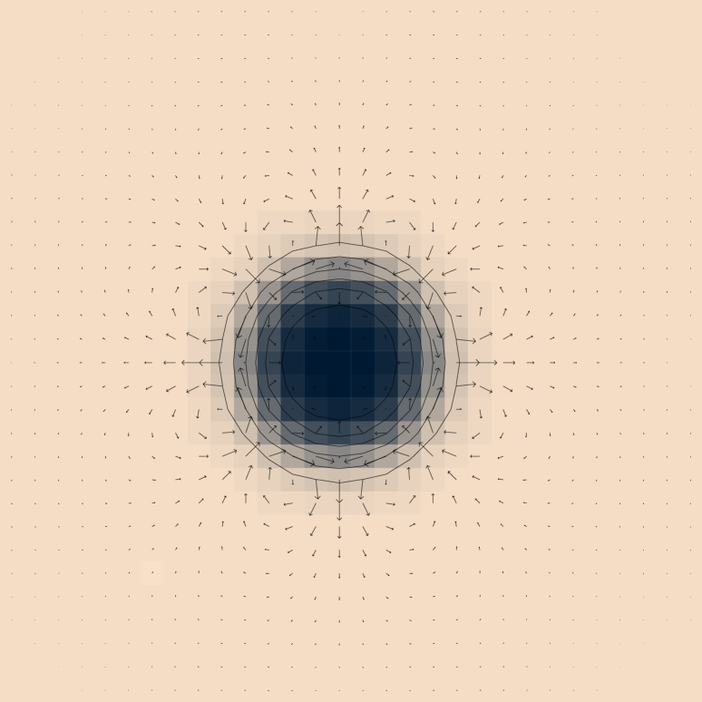
(a)

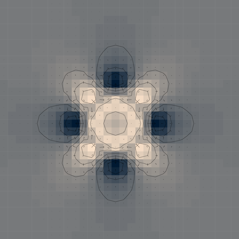
(b)

Figure 1: (a) Spurious currents for a drop where the longest velocity vector corresponds to a lattice velocity of $3.4\;10^{-4}$.The density of the matrix is $\phi=0.931$ and the density of the drop is $\phi=-1.013$. (b) The chemical potential and the spurious diffusion currents for the same drop. The longest velocity vector corresponds to a lattice velocity of $2.4\;10^{-4}$. The values of $\mu$ vary between $-1.298\;10^{-3}$ and $-1.181\;10^{-3}$.

Doing this leads to the well known spurious velocities as shown in Figure 1. We see that there are not only spurious currents but also the chemical potential $\mu$ is no longer constant. Since the implementation of a simple model B did not lead to the spurious velocities it is reasonable to assume that the implementation of the additional lattice Boltzmann equation for the total density and the momentum is the reason for the occurrence of the spurious velocities. Why should the continuous equations in equilibrium be consistent with a quiescent drop without spurious velocities? This is because the two driving terms $\nabla D\nabla\mu$ and $\nabla P^{c}$ are related through

$$\nabla\mathbf{P}^{c}=\phi\nabla\mu$$ (11)

This means that a constant chemical potential will lead to zero driving force in both equations.

When we now use this knowledge and replace the driving force $\nabla P^{c}$ with $\phi\nabla\mu$ we find that the spurious velocities vanish to machine precision. The density of the order-parameter in the surrounding fluid is $\phi=0.933$ and the density in the drop is $\phi=-1.015$ (cf Figure 1). The size of the maximum velocity is now $5.6\;10^{-16}$. The chemical potential has the value of $\mu=-1.2103\;10^{-3}$ and variations are smaller than $2\;10^{-15}$. So why do the spurious velocities appear in the first place? This is because the discretizations of $\nabla P^{c}$ and $\phi\nabla\mu$ are very different. We conclude that the different discretizations of the driving forces for the order parameter and momentum equations are the origin of spurious velocities for lattice Boltzmann.

There is, however, a caveat. The term $\phi\nabla\mu$ in its discrete form is not a divergence of a scalar field which means that momentum is now only approximately conserved. To be able to see the absence of spurious velocities I included a tiny correction term in the definition of the momentum that ensures that the total momentum of the system does not change. Also my implementation of the algorithm turned out to be unstable so I added a small amount of numerical viscosity by multiplying a velocity by $(1-0.001)$ and adding 0.00025 times the velocity of the four nearest neighbors. This rendered the simulations stable.

4 Conclusions

I proved that spurious velocities in one particular lattice Boltzmann implementation are caused by non-compatible discretizations of the driving forces for the order-parameter and momentum equations. The different discretization errors for the Forces compete and drive the spurious currents. I believe that the same argument holds for all lattice Boltzmann methods that exhibit spurious velocities. These spurious velocities can be avoided by ensuring that the discretizations of the driving forces are compatible.
Acknowledgement This work was funded by EPSRC GR/M56234 and GR/R67699.

References

- [1] R. Nourgaliev, T. Dinh, and B. Sehgal, Nucl. Eng. Des. 211, 153 (2002).
- [2] S. Teng, Y. Chen, and H. Ohashi, Int. J. Heat Fluid Flow 21, 112 (2000).
- [3] S. Hou et al., J. Comput. Phys. 138, 695 (1997).
- [4] A. Wagner, improvements for multiphase lattice Boltzmann methods (unpublished).