Magnetically mediated superconductivity: Crossover from cubic to tetragonal lattice

Abstract

We compare predictions of the mean-field theory of superconductivity for nearly-antiferromagnetic and nearly-ferromagnetic metals for cubic and tetragonal lattices. The calculations are based on the parameterisation of an effective interaction arising from the exchange of the magnetic fluctuations and assume that a single band is relevant for superconductivity. The results show that for comparable model parameters, the robustness of magnetic pairing increases gradually as one goes from a cubic structure to a more and more anisotropic tetragonal structure either on the border of antiferromagnetism or ferromagnetism.

I Introduction

One can expect that the effective interaction between quasiparticles in strongly correlated electron systems to be very complex. The interaction will depend obviously on the charge, but also more generally on the spin and current carried by the quasiparticles. On the border of long-range magnetic order it is plausible that the dominant interaction channel is of magnetic origin and depends on the relative spin orientations of the interacting quasiparticles.

It has been shown that this magnetic interaction treated at the mean field level can produce anomalous normal state properties and superconducting instabilities to anisotropic pairing states. It correctly predicted the symmetry of the Cooper state in the copper oxide superconductors[3] and is consistent with spin-triplet p-wave pairing in superfluid ${}^{3}He$ [for a recent review see, e.g., ref. [4]]. One also gets the correct order of magnitude of the superconducting and superfluid transition temperature $T_{c}$ when the model parameters are inferred from experiments in the normal state of the above systems. There is growing evidence that the magnetic interaction model may be relevant to other materials on the border of magnetism.

Thus far the magnetic interaction model has been explored in very simple cases. The most extensively investigated example is that of a nearly half-filled single-band in a square or cubic lattice. These studies have revealed a number of interesting features that are quite in contrast to those expected for conventional phonon mediated pairing. In the latter case, the interaction is local in space, but non-local in time, whereas on the border of magnetism, one expects the interaction to be strongly non-local in both space and time. For nearly antiferromagnetic metals the magnetic interaction is oscillatory in space and superconductivity depends on the ability of the electrons in a Cooper pair state to sample mainly the attractive regions of these oscillations. Because of the strong retardation in time, the relative wavefunction of the Cooper pair must be constructed from Bloch states with wavevectors close to the Fermi surface. Furthermore, the allowed symmetries of the Cooper pair wavefunction are restricted by the crystal structure. The possibility of constructing a Cooper pair state with maximum probability in the attractive regions of the magnetic interaction can be severely constrained by these requirements. Therefore, one expects that the robustness of magnetic pairing to be very sensitive to details of the electronic and lattice structures.

On the border of ferromagnetism, one is not hampered by the oscillatory nature of the magnetic interaction which in the simplest model is attractive everywhere in space and time in the spin-triplet channel. At first sight this would seem to be the most favourable case for magnetically mediated superconductivity. However, the results of the numerical calculations presented in ref. [2] indicate that the highest mean field $T_{c}$ for the cases considered is obtained for d-wave pairing in the nearly antiferromagnetic state in a quasi-2D tetragonal lattice. In this particular case, as explained in ref. [2], it turns out to be possible to ideally match the Cooper pair state to the attractive regions of the magnetic interaction.

On the border of ferromagnetism, magnetic pairing in the spin-triplet state has the disadvantage that only the exchange of magnetic fluctuations polarised along the direction of the interacting spins, i.e., longitudinal fluctuations, contribute to the quasiparticle interactions. For a spin-rotationally invariant system, both longitudinal and transverse fluctuations contribute to pairing only for a spin-singlet state.

Another disadvantage of being on the border of ferromagnetism is that for otherwise similar conditions the suppression of $T_{c}$ due to the self interaction arising from the exchange of magnetic fluctuations is stronger than in the corresponding case on the border of antiferromagnetism. This disadvantage can be mitigated in systems with strong magnetic anisotropy in that the effect of the transverse magnetic fluctuations on the self interaction would be suppressed while the strength of the pairing interaction arising from the longitudinal magnetic fluctuations need not be reduced. This may apply in systems with strong spin-orbit interactions or in the spin-polarised state close to the border of ferromagnetism.

These arguments  [1, 2] have stimulated a new search for evidence of superconductivity on the border of itinerant electron ferromagnetism in cases where spin anisotropy is expected to be pronounced, such as $UGe_{2}$. This search has proved fruitful because it led to the first observation of the coexistence of superconductivity and itinerant electron ferromagnetism in $UGe_{2}$[5] and shortly thereafter in $ZrZn_{2}$[6] and $URhGe$[7].

The prediction of the simple model presented in ref. [2] that magnetic pairing is more robust in the quasi-2D square lattice than in the cubic structure seems to have been borne out by recent experiments. Namely, one finds an order of magnitude increase in the maximum $T_{c}$ and in the range in pressure where superconductivity is observed on the border of metallic antiferromagnetism when the simple cubic lattice of $CeIn_{3}$[8] is stretched along one principal axis by the insertion of non-magnetic layers to form the tetragonal compounds $CeMIn_{5}$[9] ($M$ is $Co$, $Rh$ or $Ir$).

These systems, albeit quite anisotropic, would not normally be considered to be quasi-two dimensional and it is not clear at first sight that the model calculations carried out in ref. [2] are directly relevant. The purpose of this paper is to show that for comparable model parameters, the robustness of magnetic pairing increases gradually as one goes from a cubic structure to a more and more anisotropic structure on the border of metallic antiferromagnetism and ferromagnetism. This behaviour of the mean field transition temperature is in stark contrast to that of the ”one-loop” fluctuations corrections to $T_{c}$. The latter corrections typically depend logarithmically on the degree of anisotropy and would be expected to be negligible for materials such as $CeMIn_{5}$.

We do not expect some of the results of ref. [2] to be generic properties of the magnetic interaction model. We have already stressed that even in simple cases, the robustness of magnetic pairing can be very sensitive to certain details of the lattice and electronic structure. Even in the single band problem, many such structures have not yet been extensively studied theoretically. Furthermore, we expect that the range of possibilities to be greatly expanded in the presence of more than one partially filled electronic band.

Most known materials on the border of magnetism crystallise in other than simple cubic or tetragonal structure and have more than one band crossing the Fermi level. For these more complex systems, one would not expect the model of ref. [2] to be directly relevant. For example, the observation of spin-triplet rather than spin-singlet d-wave pairing in some multi-band materials with strongly enhanced antiferromagnetic spin fluctuations, such as $UPt_{3}$ and $Sr_{2}RuO_{4}$, may not be inconsistent with the idea of magnetic pairing. A detailed study of magnetic pairing in multi-band systems for a range of crystal structures would shed light on the possible forms of superconductivity and the conditions most favorable for their observation.

The simple model calculations suggest that anisotropic forms of superconductivity should be a generic property of systems on the border of metallic magnetism. It may seem surprising therefore that there are still so few observations of this phenomenon. In many cases, the multiplicity of bands and, for example, magnetic fluctuations in the non-bipartite lattice may weaken magnetic pairing to such an extent that quenched disorder may completely suppress superconductivity. An illustration of this point is the dramatic collapse of the spin-triplet superconducting transition temperature in $Sr_{2}RuO_{4}$ in the presence of $Al$ impurity concentrations as low as 0.1%.

At first sight, the magnetic interaction model is mathematically analogous to the conventional electron-phonon problem with the generalised magnetic susceptibility playing the role of the phonon propagator. One would therefore expect that a simple analytic expression similar to that proposed by McMillan could be used to represent approximately the $T_{c}$ calculated numerically via the Eliashberg equations. Our attempts in this direction have not, however, proved successful[1, 2]. A recent study suggests that there may be a fundamental reason for inapplicability of the McMillan-style expression for $T_{c}$[11]. On the border of long-range magnetic order, the incoherent part of the electron Green function, which is ignored in the simplest treatment, plays a major role in the formation of the Cooper pair condensate. The traditional picture in which superconductivity arose from pairing of well defined (weakly damped) quasiparticles appears inadequate on the border of metallic magnetism even in the mean field Eliashberg treatment.

We note that in our model the coupling of the quasiparticles to the magnetic fluctuations is a phenomenological constant to be inferred from normal state properties that formally includes that part of the vertex correction which is local in space and time. Calculations have shown that the neglect of vertex corrections that are non-local in space and time is justified at least in some cases of physical interest[12]. When the magnetic correlation length becomes sufficiently large, however, these neglected non-local vertex corrections (including superconducting phase fluctuations) may become important. Their effect on $T_{c}$ and the normal state properties are as yet incompletely understood.

II Model

We consider quasiparticles in a simple tetragonal lattice described by a dispersion relation

$$\epsilon_{\bf p} = -2t(\cos(p_{x})+\cos(p_{y})+\alpha_{t}\cos(p_{z}))$$ (1)

$$- 4t^{\prime}(\cos(p_{x})\cos(p_{y})+\alpha_{t}\cos(p_{x})\cos(p_{z})+\alpha_{t}\cos(p_{y})\cos(p_{z}))$$ (2)

with hopping matrix elements $t$ and $t^{\prime}$. $\alpha_{t}$ represents the electronic structure anisotropy along the z direction. $\alpha_{t}=0$ corresponds to the quasi-2D limit while $\alpha_{t}=1$ corresponds to the 3D cubic lattice. For simplicity, we measure all lengths in units of the respective lattice spacing. In order to reduce the number of independent parameters, we take $t^{\prime}=0.45t$ and a band filling factor $n=1.1$ as in our earlier work.

The effective interaction between quasiparticles is assumed to be isotropic in spin space and is defined in terms of the coupling constant $g$ and the generalised magnetic susceptibility which is assumed to have a simple analytical form consistent with the symmetry of the lattice.

$$\chi({\bf q},\omega)={\chi_{0}\kappa_{0}^{2}\over\kappa^{2}+\widehat{q}^{2}-i{\omega\over\eta(\widehat{q})}}$$ (3)

where $\kappa$ and $\kappa_{0}$ are the correlation wavevectors or inverse correlation lengths in units of the lattice spacing in the basal plane, with and without strong magnetic correlations, respectively. Let

$$\widehat{q}_{\pm}^{2}=(4+2\alpha_{m})\pm 2(\cos(q_{x})+\cos(q_{y})+\alpha_{m}\cos(q_{z}))$$ (4)

where $\alpha_{m}$ parameterises the magnetic anisotropy. $\alpha_{m}=0$ corresponds to quasi-2D magnetic correlations and $\alpha_{m}=1$ corresponds to 3D magnetic correlations.

In the case of a nearly ferromagnetic metal the parameters $\widehat{q}^{2}$ and $\eta(\widehat{q})$ in Eq. (3) are defined as

$$\widehat{q}^{2} = \widehat{q}_{-}^{2}$$ (5)

$$\eta(\widehat{q}) = T_{sf}\widehat{q}_{-}$$ (6)

where $T_{sf}$ is a characteristic spin fluctuation temperature. Note that our definition of $T_{sf}$ may differ from the characteristic spin fluctuation temperature scales used by other authors.

In the case of a nearly antiferromagnetic metal, the parameters $\widehat{q}^{2}$ and $\eta(\widehat{q})$ in Eq. (3) are defined as

$$\widehat{q}^{2} = \widehat{q}_{+}^{2}$$ (7)

$$\eta(\widehat{q}) = T_{sf}\widehat{q}_{-}$$ (8)

As in our previous work[1, 2], the band structure and generalized magnetic susceptibility are modeled independently. This choice may be inconsistent when all of the contributions to $\chi({\bf q},\omega)$ come from the chosen band. However, it allows us, in principle, to deal with the case where there are other important contributions to the generalized magnetic susceptibility. It has been argued that the latter case is of relevance to the ruthenates[10], and most likely the heavy-fermion systems.

A complete description of the model, the Eliashberg equations for the superconducting transition temperature and their method of solution can be found in the appendix.

We note that the model is fully defined by the phenomenological parameters describing the electronic structure $\epsilon_{\bf p}$, the generalised magnetic susceptibility $\chi({\bf q},\omega)$ and the interaction vertex $g$. In principle, these parameters can be estimated from experimental studies of the normal state. In particular, the resistivity can be used to estimate the dimensionless coupling parameter $g^{2}\chi_{0}/t$ the value of which is between 10 and 20 for the simplest RPA model for the magnetic interaction.

III Results

A Solution of the Eliashberg Equations for $T_{c}$

The dimensionless parameters at our disposal are $g^{2}\chi_{0}/t$, $T_{sf}/t$, $\kappa_{0}$ and $\kappa$. For comparison with the results of our earlier work[1, 2], we take $T_{sf}={2\over 3}t$ and $\kappa_{0}^{2}=12$. In 2D, this $T_{sf}$ corresponds to about $1000^{\circ}K$ for a bandwidth of 1 eV while our choice of of $\kappa_{0}^{2}$ is a representative value.

The results of our numerical calculations of the mean field critical temperature $T_{c}$ as a function of the electronic and magnetic anisotropy parameters $\alpha_{t}$ and $\alpha_{m}$, respectively, are shown in Figs 1 and 2 for representative values of the parameters $\kappa^{2}$ and $g^{2}\chi_{0}/t$. Figures 1a-c illustrate the results for a nearly anti-ferromagnetic metal and figures 2a-c for a nearly ferromagnetic metal. Note that our previous calculations correspond to the quasi-2D case $\alpha_{t}=\alpha_{m}=0$ and to 3D case $\alpha_{t}=\alpha_{m}=1$.

A glance at figure 1 reveals a clear pattern in the variation of $T_{c}$ with both anisotropy parameters $\alpha_{t}$ and $\alpha_{m}$. We notice that $T_{c}$ increases gradually and monotonically as the system becomes more and more anisotropic in either the electronic structure or in the magnetic interaction. In going from 3D to quasi-2D, $T_{c}/T_{sf}$ is found to increase by up to an order of magnitude for otherwise fixed parameters of the model. The increase becomes least pronounced as for small $\kappa^{2}$ and large $g^{2}\chi_{0}/t$.

The behavior in the nearly ferromagnetic case, figure 2, though broadly similar to that of the nearly antiferromagnetic metal, shows some interesting differences. In some cases, the minimum $T_{c}$ occurs for 3D electronic structure, but quasi-2D magnetic interaction. Also, in all cases considered the maximum $T_{c}$ is obtained for a quasi-2D electronic structure and strongly anisotropic, but not 2D magnetic interactions.

B Mass renormalisation and interaction parameter

In order to make a comparison with the corresponding electron-phonon problem it is instructive to define a mass renormalization parameter $\lambda_{Z}$ and interaction parameter $\lambda_{\Delta}$. We define

$$\lambda_{Z} = {\int_{-\infty}^{+\infty}{d\omega\over\pi}<{1\over\omega}ImV_{Z}({\bf p}-{\bf p^{\prime}},\omega)>_{FS({\bf p},{\bf p^{\prime}})}\over<1>_{FS({\bf p})}}$$ (9)

$$\lambda_{\Delta} = -{\int_{-\infty}^{+\infty}{d\omega\over\pi}<{1\over\omega}ImV_{\Delta}({\bf p}-{\bf p^{\prime}},\omega)\eta({\bf p})\eta({\bf p^{\prime}})>_{FS({\bf p},{\bf p^{\prime}})}\over<\eta^{2}({\bf p})>_{FS({\bf p})}}$$ (10)

where

$$V_{Z}({\bf q},\omega)=g^{2}\chi({\bf q},\omega)$$ (11)

and

$$V_{p}({\bf q},\omega) = -{g^{2}\over 3}\chi({\bf q},\omega)$$ (12)

$$\eta({\bf p}) = \sin(p_{x})$$ (13)

for p-wave spin triplet pairing $(\Delta\equiv p)$ while

$$V_{d}({\bf q},\omega) = g^{2}\chi({\bf q},\omega)$$ (14)

$$\eta({\bf p}) = \cos(p_{x})-\cos(p_{y})$$ (15)

in the case of d-wave spin-singlet pairing $(\Delta\equiv d)$. The Fermi surface averages are given by

$$<\cdots>_{FS({\bf p})} = \int{d^{d}p\over(2\pi)^{d}}\cdots\delta(\epsilon_{\bf p}-\mu)$$ (16)

$$<\cdots>_{FS({\bf p},{\bf p^{\prime}})} = \int{d^{d}p\over(2\pi)^{d}}{d^{d}p^{\prime}\over(2\pi)^{d}}\cdots\delta(\epsilon_{\bf p}-\mu)\delta(\epsilon_{\bf p^{\prime}}-\mu)$$ (17)

In practice, we compute the Fermi surface average with a discrete set of momenta on a cubic or tretragonal lattice and we replace the delta function by a finite temperature expression

$$\int{d^{d}p\over(2\pi)^{d}} \longrightarrow {1\over N}\sum_{\bf p}$$ (18)

$$\delta(\epsilon_{\bf p}-\mu) \longrightarrow {1\over T}f_{\bf p}(1-f_{\bf p})$$ (19)

where $f_{\bf p}$ is the Fermi function. Note that ${1\over T}f_{\bf p}(1-f_{\bf p})\rightarrow\delta(\epsilon_{\bf p}-\mu)$ as $T\rightarrow 0$. We have used $T=0.1t$ and $N=128^{d}$ in all of our calculations. The finite temperature effectively means that van Hove singularities will be smeared out.

Note that the Fermi surface average that appears in $\lambda_{Z}$, Eq. (9) plays a role similar to that of $\alpha^{2}F(\omega)/\omega$ in the case of phonon mediated superconductivity. From the definitions of the parameters $\lambda_{Z,\Delta}$ Eqs. (9),  (10) and our model for $\chi({\bf q},\omega)$ Eq. (3), we see that $\lambda_{Z,\Delta}$ are directly proportional to the dimensionless factor $g^{2}\chi_{0}\kappa_{0}^{2}/t$. Thus we will consider the quantities

$$\lambda^{*}_{Z,\Delta}\equiv\lambda_{Z,\Delta}/(g^{2}\chi_{0}\kappa_{0}^{2}/t)$$ (20)

which are functions only of $n$, $t^{\prime}/t$ and $\kappa^{2}$.

In figures 3 and 4 we show $\lambda_{Z}^{*}$, $\lambda_{\Delta}^{*}$ and the ratio $\lambda_{\Delta}/\lambda_{Z}$ for a representative value of $\kappa^{2}$ in the case of a nearly antiferromagnetic metal and nearly ferromagnetic metal, respectively.

The trends in both cases are the same. $\lambda_{Z}^{*}$ and $\lambda_{\Delta}^{*}$ are seen to increase gradually and monotonically in going from 3D to quasi-2D. However, $\lambda_{\Delta}^{*}$ grows faster than $\lambda_{Z}^{*}$ so the ratio $\lambda_{\Delta}/\lambda_{Z}$ also increases in going from 3D to quasi-2D. This qualitative trend in the ratio is consistent with the behavior of $T_{c}$ obtained from the numerical solution of the Eliashberg equations. In the ferromagnetic case, however, it fails to reproduce the fact that the minimum $T_{c}$ is not necessary for a fully 3D system and that the maximum $T_{c}$ is obtained for strongly anisotropic yet not quasi-2D systems.

IV Discussion

The results of the calculations for both the nearly ferromagnetic and nearly antiferromagnetic metals show that the robustness of magnetic pairing increases gradually as one goes from a cubic to a more and more anisotropic structure with parameters other than $\alpha_{m}$ and $\alpha_{t}$ left unchanged. These results are consistent with our previous findings [2] and with the calculations for $\alpha_{m}=\alpha_{t}=0$ and $\alpha_{m}=\alpha_{t}=1$ presented in ref. [13]. In an earlier study, Nakamura et al.  [14] found that $T_{c}$ could increase by up to a factor of three in going from 3D to 2D for their choice of model parameters. The effect of anisotropy on $T_{c}$ for nearly ferromagnetic and nearly antiferromagnetic metals is qualitatively similar. This phenomenon arises from the increase with growing anisotropy of the density of states of both the quasiparticles and of the magnetic fluctuations that mediate the quasiparticle interaction. This effect could be further enhanced in the case of a nearly antiferromagnetic metal by the change in the pattern of the oscillations of the magnetic interaction.

It can be seen from figure 5 that the strength of the interaction in the repulsive sites outside of the nodal plane of the $d_{x^{2}-y^{2}}$ state gets reduced while crucially the attraction in the basal plane gets enhanced as one goes from the cubic to a more and more anisotropic tetragonal lattice. This enhancement is the consequence of the increase of the phase space of soft magnetic fluctuations as one goes from a cubic to a quasi-two dimensional structure. Since our model potential varies smoothly with the tetragonal distortion, parameterised by $\alpha_{m}$ in figures 1 and 2, it is clear that these effects occur gradually with increasing separation between the basal planes.

The calculations assume that the maximum magnetic response for a nearly antiferromagnetic metal occurs at the commensurate wavevector defined by $Q_{x}=Q_{y}=\pi/a$ and $Q_{z}=\pi/c$, where $a$ and $c$ are the lattice constants in the basal plane and along the tetragonal axis respectively, reintroduced here for clarity. The oscillations in the magnetic interaction potential along the tetragonal axis obviously depend on the value of $Q_{z}$. However, the enhancement of the attraction in the basal plane and the reduction of the interaction elsewhere as one goes from a cubic to a more and more anisotropic lattice do not depend on the particular value of $Q_{z}$. Therefore, we expect the qualitative conclusions of this paper to be independent of $Q_{z}$.

The robustness of the pairing is further enhanced by the gradual change in the electronic band from a 3D to a quasi-2D form (see Eq. (2)). The reduced hopping along the distortion axis, parameterised by $\alpha_{t}$ in figures 1 and 2, implies a reduced electronic bandwidth and hence increased density of electronic states. Our calculations show that this too leads to a gradual increase in $T_{c}$ with increasing distortion of the lattice.

In a nearly ferromagnetic metal, one again benefits from the reduction of the electronic band width and the increase of the interaction in the basal plane as one goes from a cubic to a tetragonal lattice (see figure 6). However, the suppression of the interaction between the basal planes has a less dramatic effect on the border of ferromagnetism than antiferromagnetism because in the latter case one suppresses key repulsive regions of the interaction (figure 5).

These simple arguments explain how the pairing effects of the interaction are strengthened by a tetragonal distortion in our model. However, the same effects also contribute to an enhanced self-interaction which acts to suppress $T_{c}$. The relative importance of the pair forming and pair breaking effects of the magnetic interaction cannot be inferred by the above physical picture alone. The numerical calculations show that for most cases considered here the pair forming effects dominate. The balance is particularly delicate on the border of ferromagnetism where the suppression of $T_{c}$ brought about by the self-interaction is pronounced. A physical interpretation of this suppression of $T_{c}$ is given in ref. [11]. The same interpretation may explain, for example, why the maximum of $T_{c}/T_{sf}$ in the nearly ferromagnetic case is for a strongly anisotropic yet not quasi-2D pairing potential (figure 2).

A most striking manifestation of the interplay between the pair-forming and pair-breaking tendency of the magnetic interaction is the breakdown of the McMillan-style expression for $T_{c}$ in terms of the parameters $\lambda_{\Delta}$ and $\lambda_{Z}$ (see Eqs. (9,10). This was noted in ref. [2] and has been interpreted in ref. [11] in terms of the important role played by the incoherent part of the Green function which is ignored in the simplest treatments, but is included in the present and earlier work[1, 2] where the full momentum and frequency dependence of the self energy is taken into account.

V Outlook

The calculations show that the lattice anisotropy may increase the robustness of magnetic pairing in the mean-field approximation. Superconducting phase fluctuations which are not included in this approximation may be expected to suppress $T_{c}$ in the 2D limit. Therefore, in practice, one would think that the most favorable case for magnetic pairing is that of strong but not extreme anisotropy.

As noted in the introduction and in the previous two sections, the robustness of magnetic pairing can be very sensitive to certain details of the magnetic interaction and electronic structure. Therefore, one should exercise caution in making quantitative comparisons between the results of our calculations and experiment. For instance, one would expect all of the parameters of the model (not solely $\alpha_{m}$ and $\alpha_{t}$) to change simultaneously with increasing lattice anisotropy. The changes brought about in going from a cubic to a tetragonal lattice may even be much more complex than considered here. In particular, the number of partially filled bands may itself change. As also mentioned in the introduction, this could have in some cases even more dramatic consequences on superconductivity than the effects taken into account in our simple one-band model.

The theoretical framework developed for systems on the border of magnetism can be translated to describe systems on the border of other types of instabilities, such as charge density wave or ferroelectric instabilities. The above given phase space argument to explain the increased robustness of magnetic pairing with increasing lattice anisotropy should carry over in part to these other pairing mechanisms, at least at the one-loop mean-field level (see, e.g., ref. [15]).

While some understanding of the properties of the magnetic interaction model has been gained over the last few years (e.g., the conditions for robust pairing of electrons), there are many cases where the predictions of the model have not been worked out. Of particular importance is the role of the multiplicity of partially filled bands which may be expected to be the key to understanding exotic superconductivity observed in nearly magnetic materials such as $UPt_{3}$ and $Sr_{2}RuO_{4}$.

VI Acknowledgments

We would like to thank A.V. Chubukov, P. Coleman, S.R. Julian, P.B. Littlewood, A.J. Millis, A.P. Mackenzie, D. Pines, D.J. Scalapino and M. Sigrist for discussions on this and related topics. We acknowledge the support of the EPSRC, the Newton Trust and the Royal Society.

VII Appendix

We consider quasiparticles on a cubic or tetragonal lattice. We assume that the dominant scattering mechanism is of magnetic origin and postulate the following low-energy effective action for the quasiparticles:

$$S_{eff} = \sum_{{\bf p},\alpha}\int_{0}^{\beta}d\tau\psi^{\dagger}_{{\bf p},\alpha}(\tau)\Big{(}\partial_{\tau}+\epsilon_{\bf p}-\mu\Big{)}\psi_{{\bf p},\alpha}(\tau)$$ (22)

$$-{g^{2}\over 6N}\sum_{\bf q}\int_{0}^{\beta}d\tau\int_{0}^{\beta}d\tau^{\prime}\chi({\bf q},\tau-\tau^{\prime}){\bf s}({\bf q},\tau)\cdot{\bf s}(-{\bf q},\tau^{\prime})$$

where $N$ is the number of allowed wavevectors in the Brillouin Zone and the spin density ${\bf s}({\bf q},\tau)$ is given by

$${\bf s}({\bf q},\tau)\equiv\sum_{{\bf p},\alpha,\gamma}\psi^{\dagger}_{{\bf p}+{\bf q},\alpha}(\tau){\bf\sigma}_{\alpha,\gamma}\psi_{{\bf p},\gamma}(\tau)$$ (23)

where $\bf\sigma$ denotes the three Pauli matrices. The quasiparticle dispersion relation $\epsilon_{\bf p}$ is defined in Eq. (2), $\mu$ denotes the chemical potential, $\beta$ the inverse temperature, $g^{2}$ the coupling constant and $\psi^{\dagger}_{{\bf p},\sigma}$ and $\psi_{{\bf p},\sigma}$ are Grassmann variables. In the following we shall measure temperatures, frequencies and energies in the same units.

The retarded generalized magnetic susceptibility $\chi({\bf q},\omega)$ that defines the effective interaction, Eq. (22), is defined in Eq. (3).

The spin-fluctuation propagator on the imaginary axis, $\chi({\bf q},i\nu_{n})$ is related to the imaginary part of the response function $Im\chi({\bf q},\omega)$, Eq. (3), via the spectral representation

$$\chi({\bf q},i\nu_{n})=-\int_{-\infty}^{+\infty}{d\omega\over\pi}{Im\chi({\bf q},\omega)\over i\nu_{n}-\omega}$$ (24)

To get $\chi({\bf q},i\nu_{n})$ to decay as $1/\nu_{n}^{2}$ as $\nu_{n}\rightarrow\infty$, as it should, we introduce a cutoff $\omega_{0}$ and take $Im\chi({\bf q},\omega)=0$ for $\omega\geq\omega_{0}$. A natural choice for the cutoff is $\omega_{0}=\eta(\widehat{q})\kappa_{0}^{2}$. We have checked that our results for the critical temperature are not sensitive to the particular choice of $\omega_{0}$ used.

The Eliashberg equations for the critical temperature $T_{c}$ in the Matsubara representation reduce, for the effective action Eq. (22), to

$$\Sigma({\bf p},i\omega_{n})=g^{2}{T\over N}\sum_{\Omega_{n}}\sum_{\bf k}\chi({\bf p}-{\bf k},i\omega_{n}-i\Omega_{n})G({\bf k},i\Omega_{n})$$ (25)

$$G({\bf p},i\omega_{n})={1\over i\omega_{n}-(\epsilon_{\bf p}-\mu)-\Sigma({\bf p},i\omega_{n})}$$ (26)

$$\Lambda(T)\Phi({\bf p},i\omega_{n}) = \Bigg{[}{{g^{2}\over 3}\atop-g^{2}}\Bigg{]}{T\over N}\sum_{\Omega_{n}}\sum_{\bf k}\chi({\bf p}-{\bf k},i\omega_{n}-i\Omega_{n})|G({\bf k},i\Omega_{n})|^{2}\Phi({\bf k},i\Omega_{n})$$ (27)

$$\Lambda(T) = 1\longrightarrow T=T_{c}$$ (28)

where $\Sigma({\bf p},i\omega_{n})$ is the quasiparticle self-energy, $G({\bf p},i\omega_{n})$ the one-particle Green’s function and $\Phi({\bf p},i\omega_{n})$ the anomalous self-energy. The chemical potential is adjusted to give an electron density of $n=1.1$, and $N$ is the total number of allowed wavevectors in the Brillouin Zone. In Eq. (28), the prefactor $g^{2}/3$ is for triplet pairing while the prefactor $-g^{2}$ is appropriate for singlet pairing. Only the longitudinal spin-fluctuation mode contributes to the pairing amplitude in the triplet channel. Both transverse and longitudinal spin-fluctuation modes contribute to the pairing amplitude in the singlet channel. All three modes contribute to the quasiparticle self-energy.

The momentum convolutions in Eqs. (25,28) are carried out with a Fast Fourier Transform algorithm on a $48\times 48\times 48$ lattice. The frequency sums in both the self-energy and linearized gap equations are treated with the renormalization group technique of Pao and Bickers[16]. We have kept between 8 and 16 Matsubara frequencies at each stage of the renormalization procedure, starting with an initial temperature $T_{0}=0.6t$ and cutoff $\Omega_{c}\approx 30t$.The renormalization group acceleration technique restricts one to a discrete set of temperatures $T_{0}>T_{1}>T_{2}\dots$. The critical temperature at which $\Lambda(T)=1$ in Eq. (28) is determined by linear interpolation.

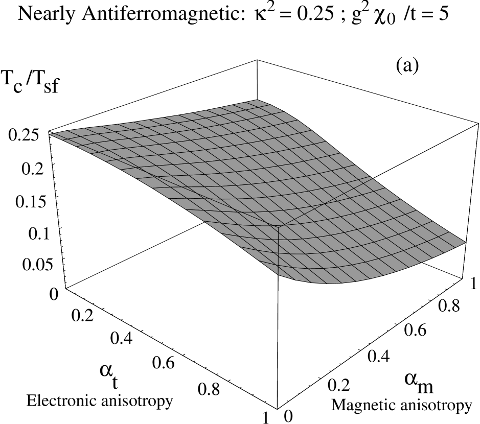
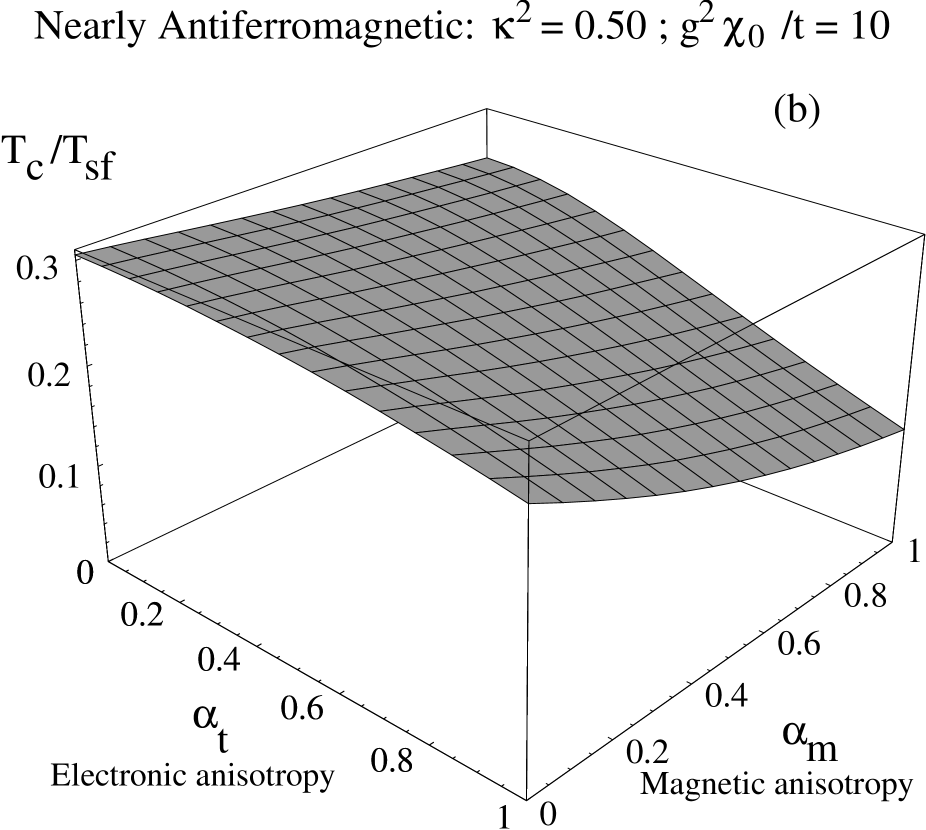
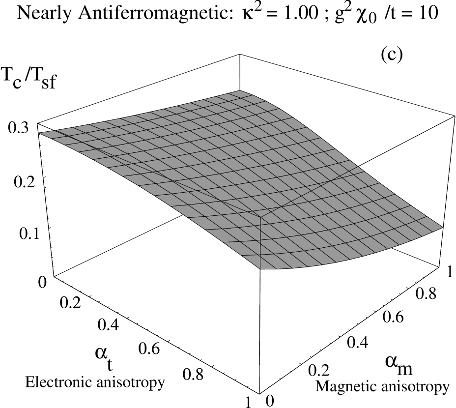
FIG. 1.: Eliashberg $T_{c}/T_{sf}$ for nearly antiferromagnetic systems as a function of the electronic anisotropy parameter $\alpha_{t}$ and the magnetic anisotropy parameter $\alpha_{m}$ for representative values of the correlation wavevector $\kappa^{2}$ and coupling constant $g^{2}\chi_{0}/t$. (a) $\kappa^{2}=0.25$, $g^{2}\chi_{0}/t=5$. (b) $\kappa^{2}=0.50$, $g^{2}\chi_{0}/t=10$. (c) $\kappa^{2}=1.00$, $g^{2}\chi_{0}/t=10$. $\alpha_{t}=\alpha_{m}=0$ corresponds to the 2D limit while $\alpha_{t}=\alpha_{m}=1$ corresponds to an isotropic 3D system.

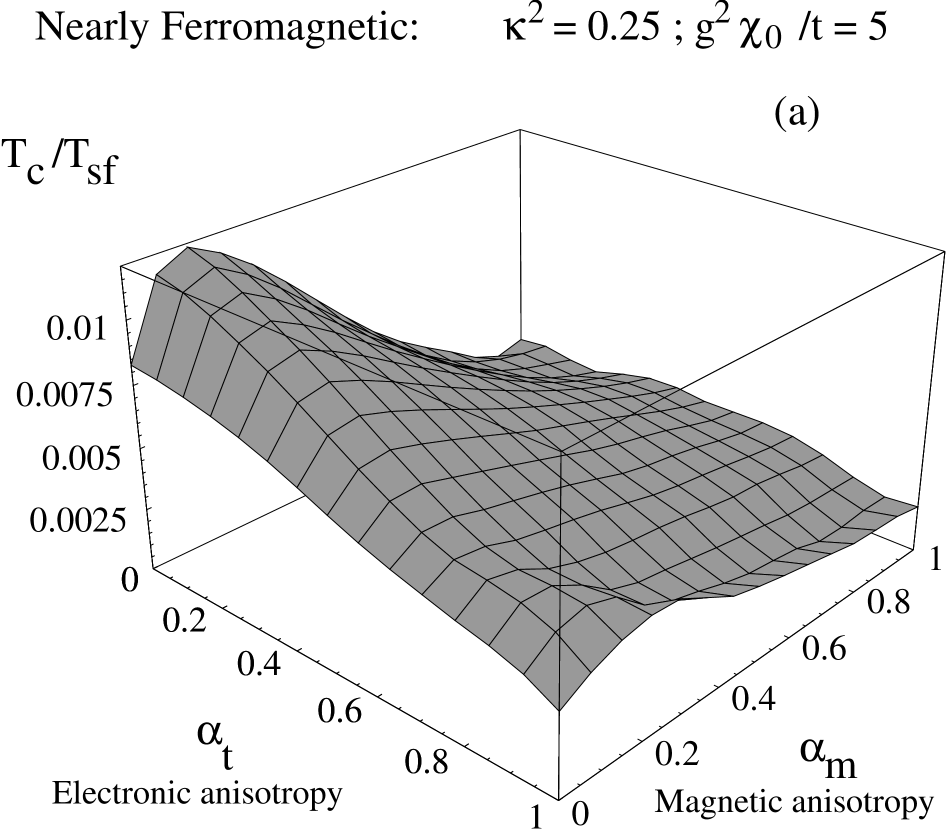
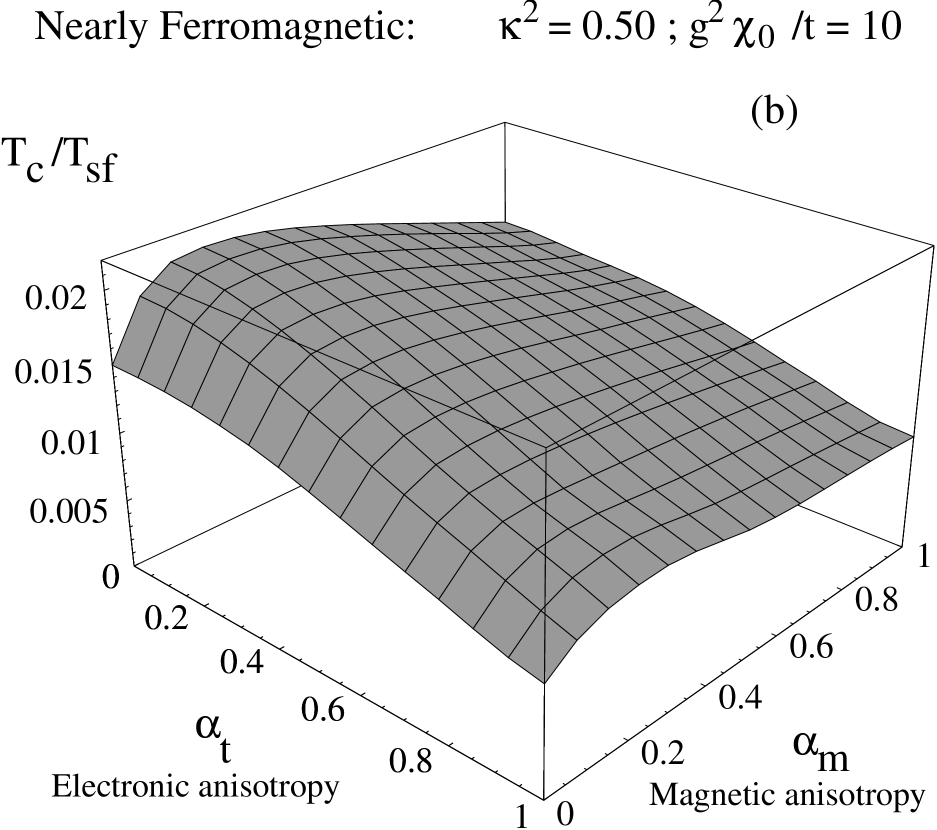
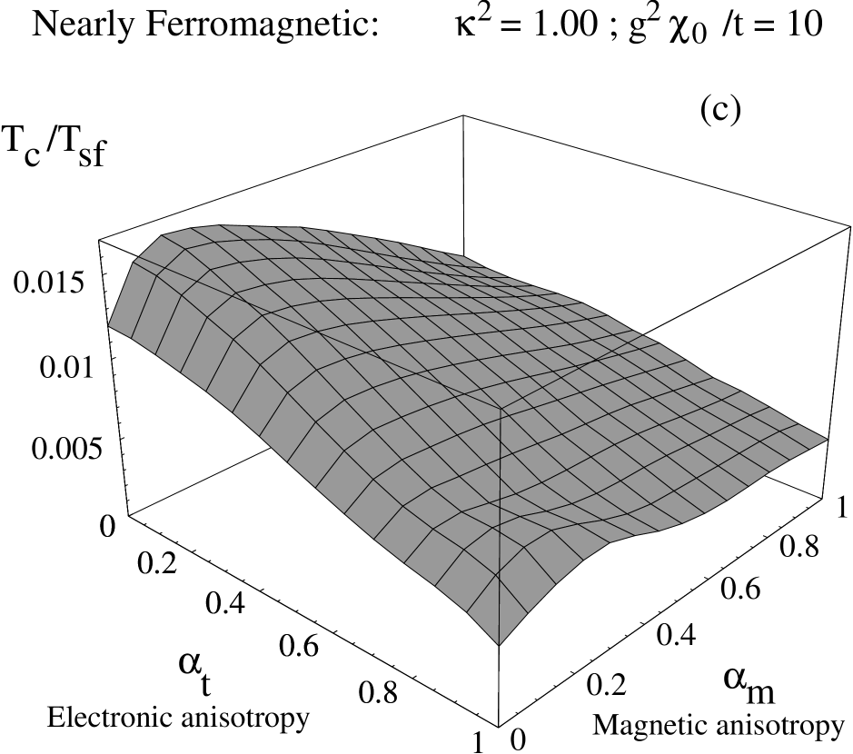
FIG. 2.: Eliashberg $T_{c}/T_{sf}$ for nearly ferromagnetic systems as a function of the electronic anisotropy parameter $\alpha_{t}$ and the magnetic anisotropy parameter $\alpha_{m}$ for representative values of the correlation wavevector $\kappa^{2}$ and coupling constant $g^{2}\chi_{0}/t$. (a) $\kappa^{2}=0.25$, $g^{2}\chi_{0}/t=5$. (b) $\kappa^{2}=0.50$, $g^{2}\chi_{0}/t=10$. (c) $\kappa^{2}=1.00$, $g^{2}\chi_{0}/t=10$. $\alpha_{t}=\alpha_{m}=0$ corresponds to the 2D limit while $\alpha_{t}=\alpha_{m}=1$ corresponds to an isotropic 3D system.

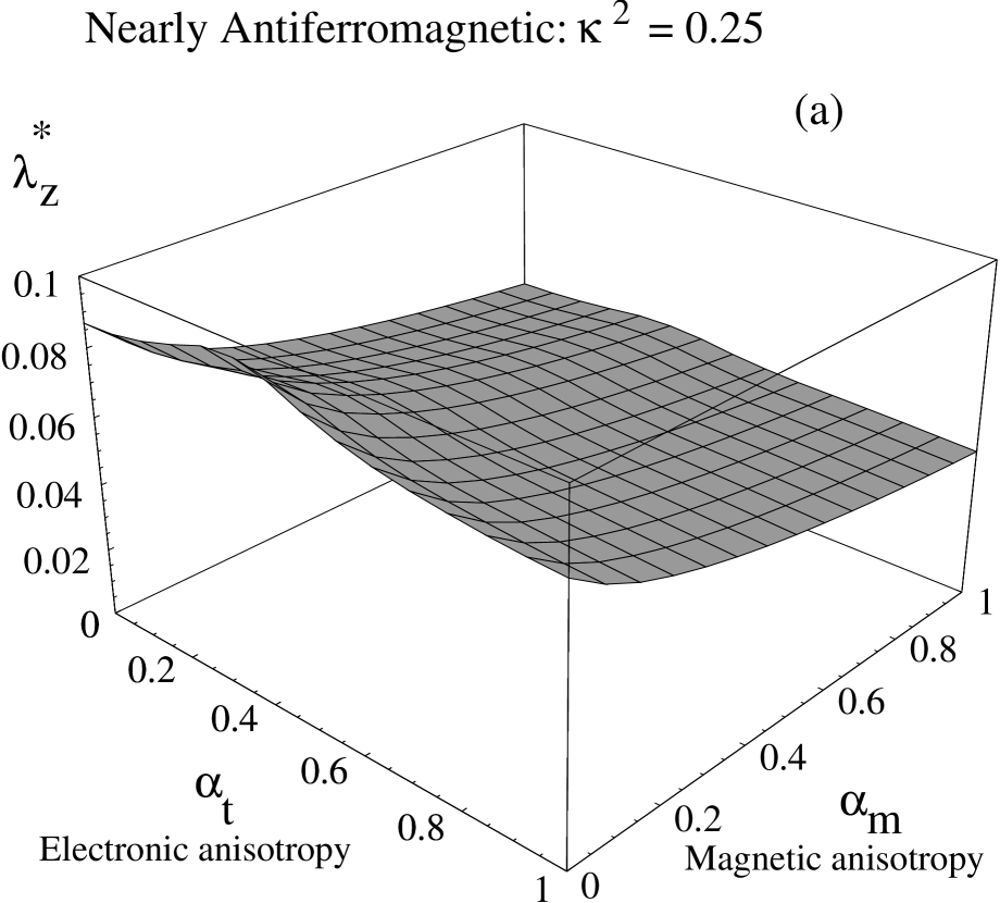
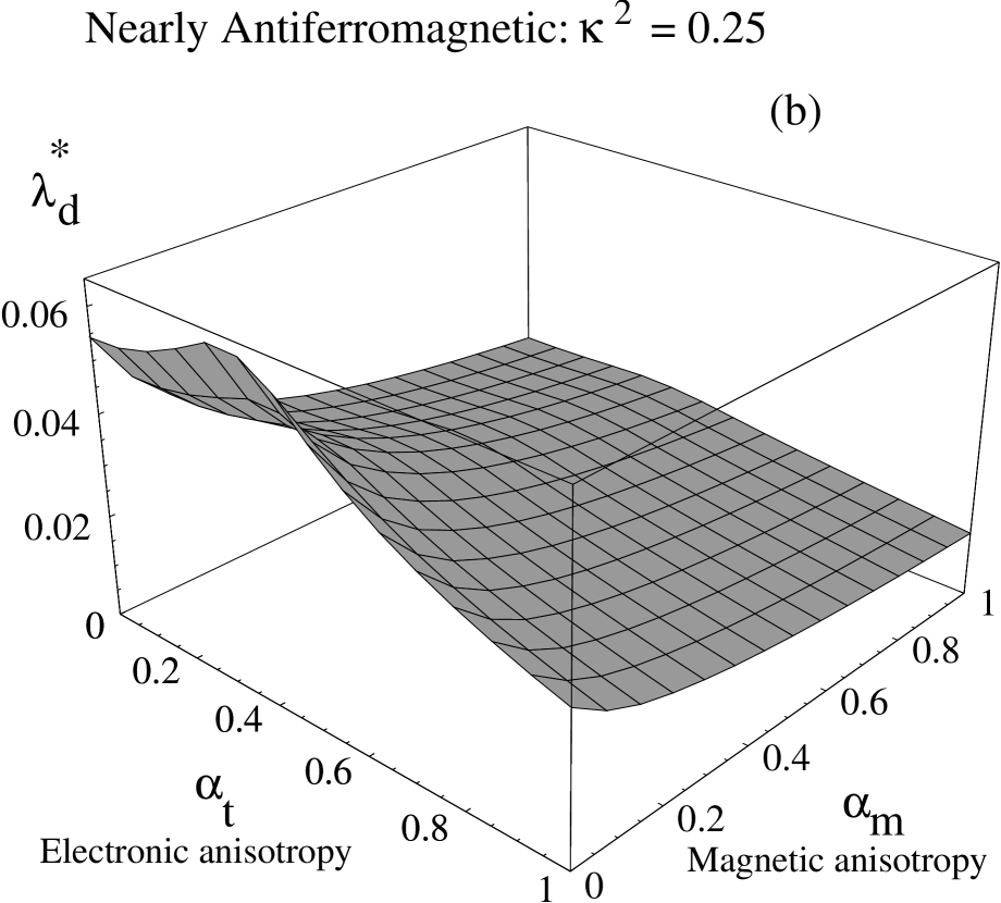
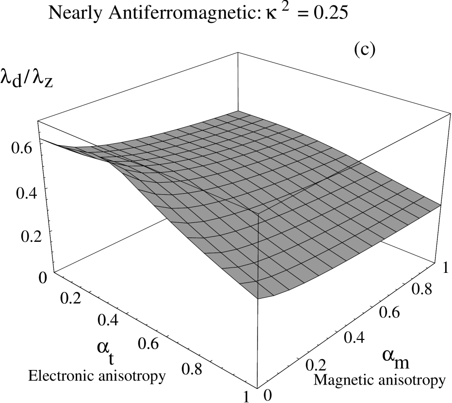
FIG. 3.: Interaction parameters (a) $\lambda_{Z}^{*}$, (b) $\lambda_{d}^{*}$ and ratio (c) $\lambda_{d}/\lambda_{Z}$ for nearly antiferromagnetic metals for a representative value of $\kappa^{2}=0.25$

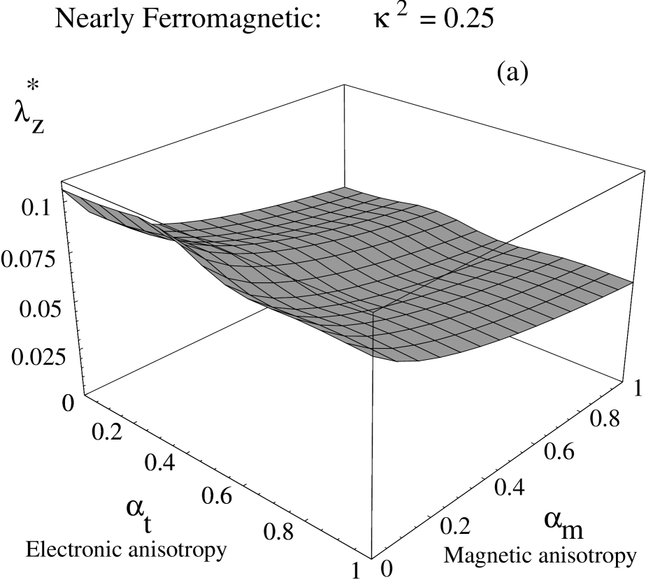
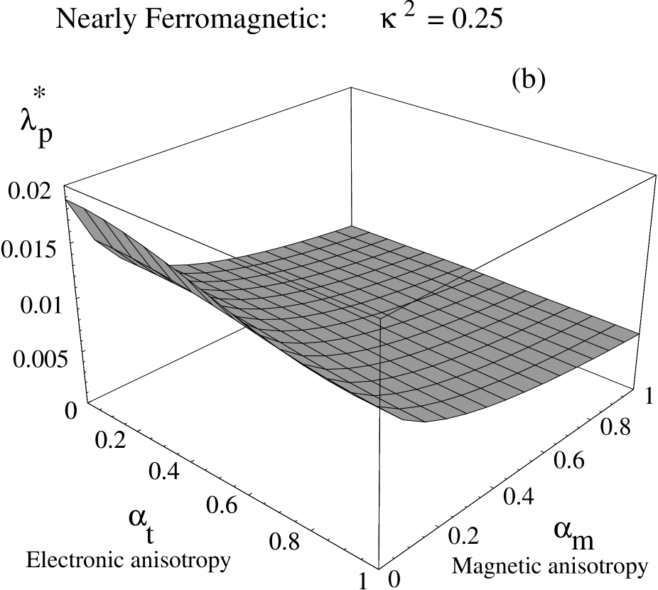
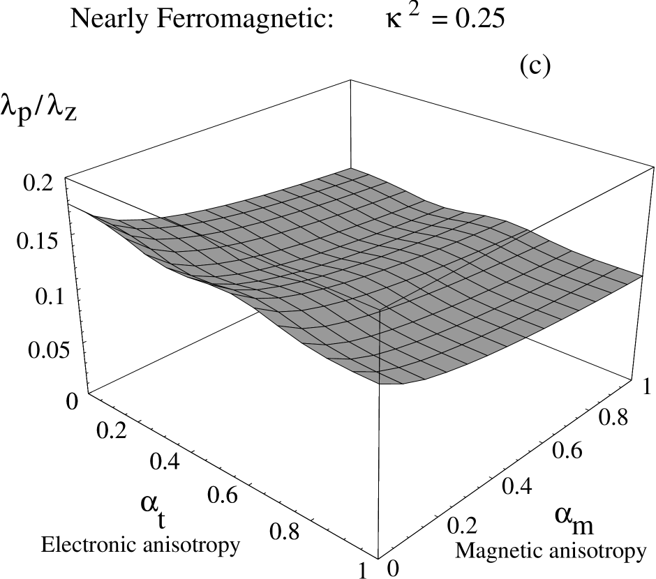
FIG. 4.: Interaction parameters (a) $\lambda_{Z}^{*}$, (b) $\lambda_{p}^{*}$ and ratio (c) $\lambda_{p}/\lambda_{Z}$ for nearly ferromagnetic metals for a representative value of $\kappa^{2}=0.25$

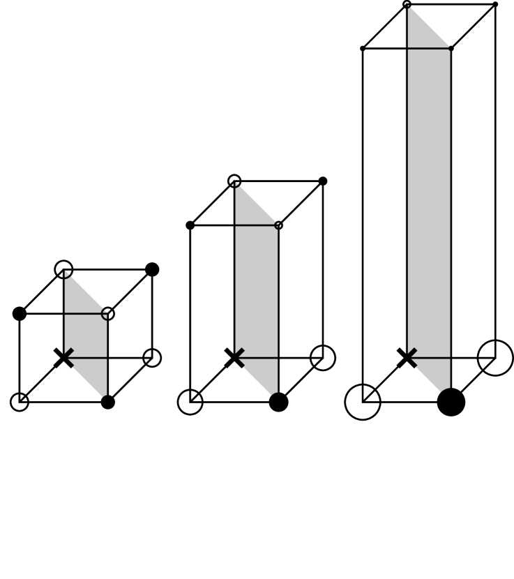
FIG. 5.: The magnetic potential seen by a quasiparticle in a spin-singlet $d_{x^{2}-y^{2}}$ Cooper pair state given that the other quasiparticle is at the origin (marked by a cross). The figure depicts the evolution of the potential as one goes from a cubic to a tetragonal lattice by varying the parameter $\alpha_{m}$. Closed circles denote repulsive sites and open circles attractive ones. The size of the circle is a measure of the strength of the interaction. The nodal plane of the $d_{x^{2}-y^{2}}$ state are represented by the shaded region.

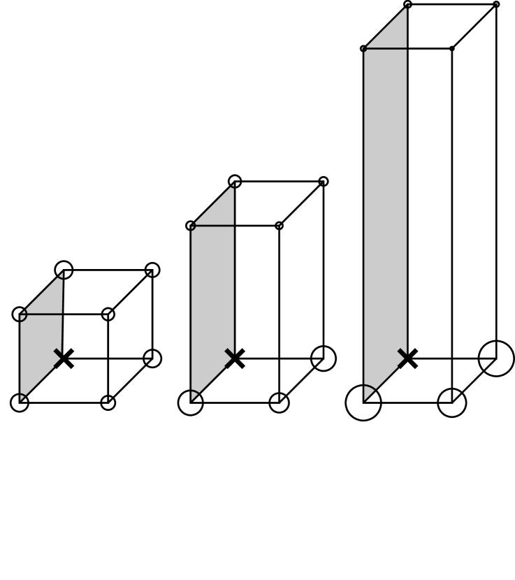
FIG. 6.: The magnetic potential seen by a quasiparticle in a spin-triplet $p_{x}$ Cooper pair state given that the other quasiparticle is at the origin (marked by a cross). The figure depicts the evolution of the potential as one goes from a cubic to a tetragonal lattice by varying the parameter $\alpha_{m}$. Open circles denote attractive sites. The size of the circle is a measure of the strength of the interaction. The nodal plane of the $p_{x}$ state is represented by the shaded region.

REFERENCES

- [1] P. Monthoux and G.G. Lonzarich, Phys. Rev. B 59, 14598 (1999).
- [2] P. Monthoux and G.G. Lonzarich, Phys. Rev. B 63, 054529 (2001).
- [3] T.Moriya, Y. Takahashi and K. Ueda, J. Phys. Soc. Jpn. 52, 2905 (1990). P. Monthoux, A.V. Balatsky and D. Pines, Phys. Rev. Lett. 67, 3448 (1991).
- [4] E.R. Dobbs, ”Helium Three”, Oxford University Press (2001).
- [5] S.S. Saxena et al., Nature 406, 587 (2000).
- [6] C. Pfleiderer et al., Nature 412, 58 (2001).
- [7] A. Aoki et al., Nature 413, 613 (2001).
- [8] I. R. Walker, F.M. Grosche, D. M. Freye, and G.G. Lonzarich, Physica C 282, 303 (1997).
- [9] C. Petrovic et al., J. Phys. C 13, L337 (2001).
- [10] T. Kuwabara and M. Ogata, Phys. Rev. Lett. 85, 4586 (2000).
- [11] A. Abanov, A.V. Chubukov, and A.M. Finkel’stein, Europhys. Lett. 54, 488 (2001).
- [12] P. Monthoux, Phys. Rev. B 55, 15261 (1997). A.V. Chubukov, P. Monthoux and D.R. Morr, Phys. Rev. B 56, 7789 (1997). P. Monthoux, Phil. Mag. B 79, 15 (1999). S. Nakamura, J.Phys. Soc. Jpn. 69, 178 (2000). N.E. Bickers and S.R. White, Phys. Rev. B 43, 8044 (1991).
- [13] R. Arita, K. Kuroki, and H. Aoki, Phys. Rev. B 60, 14585 (1999) ; J. Phys. Soc. Jpn. 69, 1181 (2000).
- [14] S. Nakamura, T. Moriya and K. Ueda, J. Phys. Soc. Jpn. 65, 4026 (1996).
- [15] I.G. Khalil, M. Teter and N.W. Ashcroft, Phys. Rev. B 65, 195309 (2002).
- [16] C.-H. Pao and N.E. Bickers, Phys. Rev. B 49, 1586 (1994).