Systematic generation of finite-range atomic basis sets for linear-scaling calculations

Abstract

Basis sets of atomic orbitals are very efficient for density functional calculations but lack a systematic variational convergence. We present a variational method to optimize numerical atomic orbitals using a single parameter to control their range. The efficiency of the basis generation scheme is tested and compared with other schemes for multiple $\zeta$ basis sets. The scheme shows to be comparable in quality to other widely used schemes albeit offering better performance for linear-scaling computations.

The last few years have seen the development of implementations of the density functional theory (DFT) Kohn and Sham (1965) in which the computer time and memory scale linearly with the number $N$ of atoms in the system studied Ordejon (1998); Goedecker (1999). These so-called order-$N$ (O($N$)) methods have increased considerably the need of accurate and efficient basis sets of finite range. While high accuracy can be achieved with flexible linear combinations of atomic orbitals (LCAO), high efficiency requires the orbitals to be as localized as possible. Numerical atomic orbitals (NAO’s) are well suited to linear scaling methods because they are very flexible, can be strictly localized, and few of them are needed for accurate results. Their main drawback is the lack of a systematic procedure to ensure a rapid variational convergence with respect to the number of basis orbitals and to the range and shape of each orbital.

In the context of the ab initio pseudopotential method for solids, an early proposal were the ‘fireballs’ of Sankey and Niklewski: solutions of the radial Schrödinger equation for an isolated pseudo-atom confined in a spherical hard potential box Sankey and Niklewski (1989). Subsequent works proposed different recipes to find multiple-$\zeta$ and polarization orbitals Lippert et al. (1996); Artacho et al. (1999); Soler et al. (2002). In a recent work Junquera et al. (2001), a method was proposed to optimize the shape of the orbitals by substituting the hard box by a soft confining spherical potential Porezag et al. (1995); Horsfield (1997); Junquera et al. (2001). This confining potential, which may be different for each atomic orbital, depends on a series of parameters which determine the orbital’s shape. The parameters are then adjusted to minimize the energy of a prototype molecule or solid. If the confining potentials diverge at given cutoff radii, the orbitals become strictly zero beyond those radii. However, if the cutoff radii themselves are included as variational parameters, without constraints to impose a small range, the resulting orbitals tend to become very extended, with long tails that generally have no particular significance for the condensed system, but which limit severely their efficiency. In the present work, we propose a simple procedure to compress the orbital radii by introducing a fictitious pressure. This allows to balance efficiency versus accuracy in a continuous and well controlled way. In addition, we evaluate the variational completeness of the resulting orbital shapes, by adding additional degrees of freedom, and by exploring alternative generation procedures and comparing their relative merits.

Our basis orbitals are products of spherical harmonics times numerical radial functions centered on atoms. The quantum chemistry literature typically distinguishes between core, valence, polarization, and diffuse basis orbitals. In our case, core states are eliminated by the use of norm-conserving pseudopotentials Troullier and Martins (1991). The explicit description of semicore electrons as valence is performed with the same methods described here, but using a pseudopotential for which the semicore electrons occupy the ground state and the valence electrons occupy the first excited state (with a radial node). In previous works we have designed a specific numerical method for polarization orbitals Soler et al. (2002), but here we will use the same methods for valence and polarization orbitals. We will not consider diffuse orbitals in this work.

When several basis orbitals with the same center and angular momentum are used to expand the valence states, we follow the standard quantum chemical terminology and call them first-$\zeta$ orbital, second-$\zeta$ orbital, etc, even though there are no $\zeta$ exponent coefficients in our orbitals. We use a different method to generate the first-$\zeta$ orbitals than that for the subsequent-$\zeta$ orbitals. For the first-$\zeta$ orbitals we solve the radial Schrödinger equation for a potential given by the sum of the full (screened) nonlocal pseudopotential corresponding to the angular momentum of the orbital, and a confining potential of the form $V(r)=V_{\rm o}\exp\left[-(r_{c}-r_{i})/(r-r_{i})\right]/(r_{c}-r)$ which depends on three parameters $r_{i}$, $V_{0}$, and the cutoff radius $r_{c}$. These parameters are different for each basis orbital and define its range as well as its shape by allowing a depression of the tail. Other confinement schemes have been proposed Sankey and Niklewski (1989); Porezag et al. (1995); Horsfield (1997) and are compared with this one in Ref. [Junquera et al., 2001]. To generate the second and subsequent-$\zeta$ orbitals we will use and compare two possible methods. The first one is based on the concept of chemical hardness (CH) and defines the different-$\zeta$ orbitals as the derivatives of the ground-state wavefunction of the potential (pseudo plus confining) with respect to the charge of the atom Lippert et al. (1996). In this scheme, there are no independent parameters to fix the shape of the higher-than-first-$\zeta$ orbitals.

The second scheme to generate higher-$\zeta$ orbitals was inspired by the “split valence” (SV) method which is standard in quantum chemistry, where orbitals are given by fixed linear combination of gaussians Huzinaga et al. (1984). The second-$\zeta$ (or triple etc) orbitals are obtained by “splitting” the slowest-decaying gaussian(s) to act as independent basis orbital(s). The SV was adapted to numerical atomic orbitals by constructing a double-$\zeta$ orbital as one that reproduces the tail of the first-$\zeta$ from a matching radius outwards, and runs smoothly inwards Artacho et al. (1999); Junquera et al. (2001); Soler et al. (2002). Higher-$\zeta$ orbitals are obtained repeating the procedure at different radii.

A variational optimization of a basis set constructed as described above can give orbitals with too long cutoff radii $r_{c}$. In order to reduce their range in a systematic way we introduce a parameter $P$ with dimensions of pressure (that we will call “pressure” henceforth) and minimize the “enthalpy” $E+PV$, where $E$ is the total energy of some reference system and $V=(4\pi/3)\sum_{\mu}r^{3}_{c\mu}$ is the sum of the volumes of the basis orbitals $\phi_{\mu}$. The convergence of calculated properties with respect to orbital range is thus controlled by a single parameter, much in the same way as the planewave cutoff controls the convergence of a plane wave basis set.

The reference system for which $E+PV$ is minimized is a molecule or solid in which the atoms considered have a prominent role, and which is small enough to allow many selfconsistent calculations with different basis parameters. The derivatives of $E$ with respect to those parameters are generally not available, and we use the downhill-simplex methodPress et al. (1992) to minimize it. The basis orbitals depend on the described parameters in a non-linear way, and several local minima are found in many cases. This is to be expected because different combinations of parameters can produce approximately the same optimal shape. Since our parameters have no special physical significance, any low local minimum is in principle equally acceptable, even though the multiple minima produce a somewhat unpleasant “noise” in the results reported below.

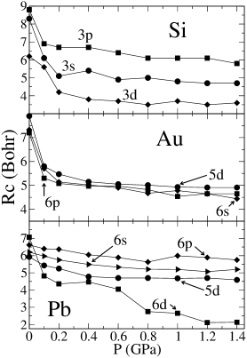
Fig. 1, shows the cutoff radii of the first-$\zeta$ orbitals of Si, Au, and Pb as a function of the pressure parameter $P$. The basis optimizations were performed in their corresponding bulk solids, with a so-called double-$\zeta$ polarized (DZP) basis set: in Si there are double-$\zeta$ $s$ and $p$ shells and single-$\zeta$ $d$ orbitals; in Au there are double-$\zeta$ $s$ and $d$, and single-$\zeta$ $p$; in Pb the $5d$ semicore electrons are included in the valence as double-$\zeta$, as are the $s$ and $p$ shells, while the $6$d have a single-$\zeta$. The second-$\zeta$ orbitals were generated with the SV scheme. Polarization orbitals are obtained in the same manner as the other atomic orbitals.

Figure 1: Cutoff radii of the first-$\zeta$ basis orbitals of Si, Au and Pb, as a function of the fictitious pressure parameter $P$

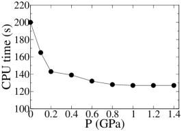
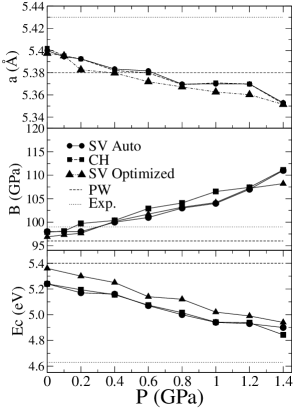
To give an idea of how the orbital radii affect the basis efficiency, Fig. 2 shows the CPU time required for the calculation of a selfconsistent step of bulk silicon, as a function of the pressure $P$ used to generate the basis. The accuracy of the results, as the orbitals contract, is addressed in Table LABEL:aBEc, which shows the variation in lattice parameter, bulk modulus, and cohesive energy with $P$. The results were obtained using the Siesta method Sanchez-Portal et al. (1997); Soler et al. (2002), with a well converged real-space integration grid. They are compared to experiment and to well-converged plane wave calculations, performed with a specific program designed to use exactly the same pseudopotential Troullier and Martins (1991); Kleinman and Bylander (1982), exchange correlation functional Perdew and Zunger (1981), and $k$-grid sampling Monkhorst and Pack (1976) used in Siesta. The cohesive energy is calculated as the difference between the bulk total energy per atom (with the chosen basis set) and an atomic calculation in which the radial Schrödinger equation is solved numerically, without any constraint to the shape or range of the orbitals. With this definition the cohesive energy carries the variational character of the total energy (higher binding energies for better basis sets).

Figure 2: CPU time for a selfconsistency step of bulk Si (16 atoms per cell) versus the fictitious pressure $P$ used to compress the cutoff radii of the DZP basis orbitals.

Table 1: Comparison of structural properties of different systems as a function of the pressure parameter $P$ (in GPa) used to generate their basis sets. Lattice parameters $a$ in Å, bulk moduli $B$ in GPa and cohesive energies $E_{c}$ in eV. The bulk moduli were obtained by fitting the total energy with a Murnaghan equation of state Murnaghan (1944). A double-$\zeta$ plus polarization basis was used in all cases. In Pb semicore states where also used.

		Exp	PW	P=0	0.2	0.4	0.8	1.2	1.4
Si	$a$	5.43	5.38	5.40	5.38	5.38	5.37	5.36	5.35
	$B$	99	96	97	98	100	103	107	108
	$E_{c}$	4.63	5.40	5.36	5.30	5.25	5.12	4.99	4.94
Au	$a$	4.08	4.05	4.06	4.06	4.05	4.02	4.02	4.00
	$B$	195	198	206	210	211	220	239	242
	$E_{c}$	4.13	4.36	4.04	3.96	3.95	3.80	3.77	3.66
Pb	$a$	4.95	4.88	4.90	4.87	4.83	4.79	4.81	4.80
	$B$	43	54	54	60	64	71	70	75
	$E_{c}$	2.04	3.77	3.68	3.63	3.48	3.37	3.32	3.29
MgO	$a$	4.21	4.10	4.11	4.10	4.10	4.11	4.09	4.06
	$B$	152	164	182	205	209	205	214	230
	$E_{c}$	10.30	12.39	12.18	12.10	12.00	11.86	11.92	11.66

It can be seen that a moderate pressure of $\sim 0.2$ GPa produces a drastic reduction of the orbital radii, with a correspondingly large reduction of CPU time, without a significative change in the results. Larger pressures produce additional, though more moderate gains in basis efficiency, but at the expense of nonneglegible changes in the results. That small pressure of 0.2 GPa seems to be a threshold up to which only the very low, not significant, tails are removed.

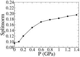
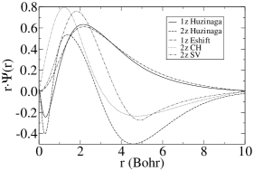
The relative merits of the SV and CH methods to generate the second-$\zeta$ orbitals are considered in Fig. 3. For the SV case, two curves are plotted. In one of them, the inner matching radius of the sencond-$\zeta$ orbitals is optimized for every value of $P$. In the other one, it is determined by a standard automatic criterion Soler et al. (2002), by which the norm of the first-$\zeta$ orbital beyond the matching radious has to be equal to a given “split-norm” parameter value of 0.15. Fig. 4 shows the optimized value of this parameter, which does not differ much from the standard value. As a consequence, it is not surprising that Fig. 3 shows a similar quality of the results using the optimized and standard values. The quality is also similar for the CH method, which does not depend on any variational parameter. Again, this is not surprising, in view of the similarity of the resulting shapes of the second-$\zeta$ orbitals, which are compared in Fig. 5 to our SV orbitals and to a typical quantum-chemistry gaussian-based polarization orbital Huzinaga et al. (1984). We may then conclude that the different generating schemes of second-$\zeta$ orbitals compared here yield basis sets of similar quality. Our SV scheme, however, offers higher efficiency for linear-scaling computations since the range of the higher-$\zeta$ orbitals may be restricted to their inner matching radius, without any reduction of the variational freedom Soler et al. (2002).

Figure 3: Equilibrium lattice constant ($a$), bulk modulus ($B$) and cohesive energy ($Ec$) of bulk Silicon as a function of the fictitious pressure parameter $P$. A double-$\zeta$ plus polarization basis was used. The second-$\zeta$ orbitals were generated using the chemical-hardness (CH) and split-valence (SV) schemes. For the latter, results are shown for orbitals whose inner matching radii were generated with a constant split-norm parameter of 0.15 or optimized variationally for each value of $P$ (what resulted in the split-norm parameters shown in Fig. 4).

Figure 4: Optimal value of the split-norm parameter, which determines the inner matching radius of the second-$\zeta$ orbitals of silicon generated with the split-valence scheme.

Figure 5: Radial shape of the first and second $\zeta$ $p$-orbitals of Si. The second-$\zeta$ orbital was generated using the chemical-hardness (CH) and split-valence (SV) approaches described in the text. In addition, we show the second-$\zeta$ gaussian orbital of Huzinaga Huzinaga et al. (1984). The second-$\zeta$ orbitals have been orthogonalized to the first-$\zeta$ one to facilitate the comparison.

Finally, we explore to what extent the orbital shapes generated with the described schemes differ from optimal. To this end, we have added spherical Bessel functions to our generated orbitals, not as additional basis functions but to change the shape of the orbitals in a DZP basis, introducing the coefficients of the linear combination as the parameters to be optimized. Table 2 shows the effect in the total energy for bulk silicon. as subsequent Bessel functions are added to optimize different orbitals. The energy reduction is quite moderate, and considerably smaller than that obtained by introducing additional basis orbitals. This is true even in the case of the higher-$\zeta$ orbitals, whose shape depends on just one parameter. It can be thus concluded that the radial shapes of the basis orbitals are indeed well optimized by the variational freedom contained in the confining potential, and by the physically motivated schemes used to generate the higher-$\zeta$ orbitals.

Basis Size	$\Delta E$ (meV)
DZP not optimized	230
DZP optimized	40
DZP 4 Bessels in first $\zeta$	33
DZP 4 Bessels in second $\zeta$	33
DZP + F	22
DZ2P + F	16

Table 2: Test of the quality of the DZP optimized basis set of silicon. Second-$\zeta$ orbitals were generated with the split-valence method. The energies $\Delta E$ are per atom and relative to the converged plane wave result. The F stands for the addition of a $f$ angular momentum shell. The 2 in the DZ2P denotes the addition of a second $\zeta$ to the $d$ polarization orbital. The non-optimized basis was obtained with a hard potential Sankey and Niklewski (1989) (the radii are as long as in the DZP optimized case) and a standard split-norm parameter of 0.15. A zero pressure parameter $P$ was used in all the cases.

In conclusion, we have developed a systematic method to construct accurate and efficient atomic basis orbitals for linear-scaling DFT calculations. The range of the basis sets is controlled by a single parameter, that allows to monitor their convergence with range in a simple and systematic way. By comparing different generation schemes, and by studying the effect of additional variational freedom, we have found that our method produces nearly optimal shapes in multiple-$\zeta$ polarized basis sets.

We thank Pablo Ordejón, Alberto García, Daniel Sánchez-Portal, and Eduardo Hernández for useful discussions. This work was supported by the Fundación Ramón Areces and by Spain’s MCyT grant BFM2000-1312.

References

- Kohn and Sham (1965) W. Kohn and L. J. Sham, Phys. Rev. 140, A1133 (1965).
- Ordejon (1998) P. Ordejon, Comp. Mat. Sci. 12, 157 (1998).
- Goedecker (1999) S. Goedecker, Rev. Mod. Phys. 71, 1085 (1999).
- Sankey and Niklewski (1989) O. F. Sankey and D. J. Niklewski, Phys. Rev. B 40, 3979 (1989).
- Lippert et al. (1996) G. Lippert, J. Hutter, P. Ballone, and M. Parrinello, J. Phys. Chem. 100, 6231 (1996).
- Artacho et al. (1999) E. Artacho, D. Sanchez-Portal, P. Ordejon, A. Garcia, and J. M. Soler, Phys. Stat. Sol. (b) 215, 809 (1999).
- Soler et al. (2002) J. M. Soler, E. Artacho, J. Gale, A. Garcia, J. Junquera, P. Ordejon, and D. Sanchez-Portal, J. Physics: Condensed Matter 14, 2745 (2002).
- Junquera et al. (2001) J. Junquera, O. Paz, D. Sanchez-Portal, and E. Artacho, Phys. Rev. B 64, 235111 (2001).
- Porezag et al. (1995) D. Porezag, T. Frauenheim, T. Köhler, G. Seifert, and R. Kaschner, Phys. Rev. B 51, 12947 (1995).
- Horsfield (1997) A. P. Horsfield, Phys. Rev. B 56, 6594 (1997).
- Troullier and Martins (1991) N. Troullier and J. L. Martins, Phys. Rev. B 43, 1993 (1991).
- Huzinaga et al. (1984) S. Huzinaga et al., Gaussian basis sets for molecular calculations (Elsevier Science, Berlin, 1984).
- Press et al. (1992) W. H. Press, S. A. Teukolsky, W. T. Vetterling, and B. P. Flannery, Numerical Recipes (Cambridge University Press, Cambridge, 1992).
- Sanchez-Portal et al. (1997) D. Sanchez-Portal, P. Ordejon, E. Artacho, and J. M. Soler, Int. J. Quantum Chem. 65, 453 (1997).
- Kleinman and Bylander (1982) L. Kleinman and D. M. Bylander, Phys. Rev. Lett. 48, 1425 (1982).
- Perdew and Zunger (1981) J. P. Perdew and A. Zunger, Phys. Rev. B 23, 5048 (1981).
- Monkhorst and Pack (1976) H. J. Monkhorst and J. D. Pack, Phys. Rev. B 13, 5188 (1976).
- Murnaghan (1944) F. D. Murnaghan, Proc. Natl. Acad. Sci. 30, 244 (1944).