Schematic models for dynamic yielding of sheared colloidal glasses

Abstract

  The nonlinear rheological properties of dense suspensions are discussed within simplified models, suggested by a recent first principles approach to the model of Brownian particles in a constant-velocity-gradient solvent flow. Shear thinning of colloidal fluids and dynamical yielding of colloidal glasses arise from a competition between a slowing down of structural relaxation, because of particle interactions, and enhanced decorrelation of fluctuations, caused by the shear advection of density fluctuations. A mode coupling approach is developed to explore the shear-induced suppression of particle caging and the resulting speed-up of the structural relaxation.  

I Introduction

Soft materials, such as particle dispersions, exhibit a wide range of rheological properties. While dilute colloids flow with a viscosity only slightly higher than that of the solvent, concentrated dispersions behave as weak amorphous solids. For intermediate concentrations, one generally observes, upon increasing the external shear rate, first, a strong decrease of the dispersion viscosity (“shear thinning”), and then an (often dramatic) increase of the viscosity (“shear thickening”) larson ; russel .

While shear-induced crystallization of particle suspensions causes a marked decrease of the viscosity, shear thinning is not always accompanied by a flow-induced ordering Laun92 ; Bender96 ; Strating99 ; Foss00 , but appears connected more generally to a decrease of the Brownian contribution to the stress Brady96 ; Bergenholtz01b . In concentrated suspensions of polydisperse colloidal particles the structure remains amorphous during the application of shear but still exhibits shear thinning or yield behaviour Petekidis02 ; Petekidis02b .

Detailed light scattering studies of quiescent colloidal hard sphere suspensions Megen91 ; Megen94 ; Beck99 ; Bartsch02 have identified a slowing down of the structural relaxation as the origin of the solid-like behavior at high concentrations. Operationally, a transition to an amorphous solid or glass can be defined when the structural relaxation time increases beyond the experimental observation time, and various concomittant signatures of metastability have been observed. The resulting amorphous solids, even though their life-time may be limited by aging and crystallisation processes, nevertheless were found to possess a well defined average arrested structure. On the theoretical side, predictions for the glassy structure and the slow-down of the structural relaxation have been obtained within the mode coupling theory (MCT), which describes an idealized glass transition scenario with a divergent structural relaxation time at a critical concentration (or temperature) Bengtzelius84 ; Goetze91b ; gs . Comparisons of theory and experimental data have shown agreement on the 30% relative error level Megen91 ; Megen94 ; Beck99 ; Bartsch02 ; Goetze99 .

Considering that arrested systems like collidal glasses often are redispersed by shaking or stirring the sample, the influence of external shear strain or stress on glasses obviously is of interest. Because glass formation is connected to a growing internal relaxation time, an important aspect of the imposition of external driving is the introduction of new time scales. In the case of steady shearing, this aspect is generally discussed as interplay of shear-induced and Brownian motion. Because, without shear, the glassy system fails to reach equilibrium for long times, it is unclear to which stationary non-equilibrium state shear motion leads, and how this non-equilibrium state approaches the equilibrium one in the limit of vanishing shear rate. Various phenomenological models (“constitutive equations”) either describe a yield-stress discontinuity (Bingham plastic, Hershel-Bulkeley law), or a power-law approach (power-law fluid) larson , while recent glass theories predict the former Fuchs02 , the latter Berthier00 , or a transition from one to the other with concentration or temperature Fielding00 .

In order to gain more insight into the yielding of colloidal glasses and the nonlinear rheology of colloidal fluids, we extend here the analysis of the microscopic approach which we recently presented Fuchs02 . We derive from it simplified models, aiming to bring out the qualitative and universal features. A simple case of non-linear rheology is studied: a system of Brownian particles in a prescribed steady shear solvent flow with constant velocity gradient. While hydrodynamic interactions and fluctuations in the velocity profile are thus neglected from the outset, this (microscopic) model has the advantage that the equation of motion for the temporal evolution of the many-particle distribution function can be written down exactly russel ; dhont . Our theoretical development can therefore be crucially tested by Brownian dynamics simulations, like Ref. Strating99 , and constitutes a first microscopic approach to real glassy colloidal suspensions. The properties of this microscopic model have been worked out for low densities Blawzdziewicz93 ; Bergenholtz01c and it provides the starting point for various (approximate) theories for intermediate concentrationsLionberger00 .

II Microscopic approach

The effect of a constant uniform shear rate $\dot{\gamma}$ on the particle dynamics is measured by the Peclet number russel , Pe${}_{0}=\dot{\gamma}d^{2}/D_{0}$, formed with the bare diffusion coefficient $D_{0}$ of a particle of diameter $d$. If the quiescent systems exhibits a much longer time scale $\tau$, as do dense colloidal suspensions where $\tau$ is the final or structural relaxation time, then a second, “dressed” Peclet (or Weissenberg) number, Pe $=\dot{\gamma}\tau$, can be defined. This characterizes the influence of shear on the structural relaxation and increases without bound at the glass transition, even while Pe${}_{0}\ll 1$. In Ref. Fuchs02 , we argued that the competition of structural rearrangement and shearing that arises when Pe $>1\gg$ Pe₀ dominates the non-linear rheology of colloids near the glass transition.

While the time scale ratios Pe₀ and Pe appear quite generally, the physical mechanisms active when Pe $>1$ may be quite different for different classes of soft matter. As we argued in the introduction, flow-induced ordering shall here be assumed absent. In the quiescent dispersion, the structural relaxation is dominated by (potential) particle interactions which either cage Bengtzelius84 or bond Bergenholtz99 a central particle among its neighbours. Either mechanism leads to a slowing down of particle rearrangements accompanied by growing memory effects. The former process (“cage-effect”) is driven by the local order as measured in the height of the principal peak of the static structure factor, $S_{q_{p}}$, and leads to a prolonged decay-time of especially this density mode; note that its wavevector $q_{p}$ is inversely related to the average particle spacing. The decay time of this dominant cage mode sets the structural relaxation time $\tau$, which in the following shall be defined by $\Phi_{q_{p}}(t/\tau)=0.1$, where $\Phi_{q}(t)$ is the normalized intermediate scattering function.

It is important to realize that during the time interval so defined a single particle has diffused (in direction $x$, say) a fraction of its size onlyMegen94 ; Megen98 ; Fuchs98 : $\langle\Delta x^{2}(\tau)\rangle\approx 0.1d^{2}$. In the sheared system at Pe $=1$, therefore, it is not true that kinetic flow of the particle with the solvent (“Taylor dispersion” which would give $\langle\Delta x^{2}(t)\rangle=\frac{2}{3}D_{0}\dot{\gamma}^{2}t^{3}$ along the flow direction dhont ) has displaced the particles relative to each other during the time interval $t=\tau$. This would imply a rapid destruction of the cage already for Pe $\leq 1$. Rather, the effect of shear on the structural relaxation has to be sought in its effect on the cage mode, i.e., the collective density fluctuations with wavevector $q_{p}$. Because the steady state structure factor differs only smoothlyBender96 ; Berthier02 ; Laun92 ; dhont from the quiescent $S_{q}$ around $q\approx q_{p}$ for Pe${}_{0}\ll 1$, the effect of shear cannot lie in a destruction of the steady state local order. This would require larger Peclet numbers and contradict the notion that an infinitesimal steady shear rate melts a glass. Rather, the effect needs to arise from a shear-induced decorrelation of the memory built up in the collective cage mode. The likely mechanism thus appears to be the shear advection of fluctuations dhont ; Onuki79 .

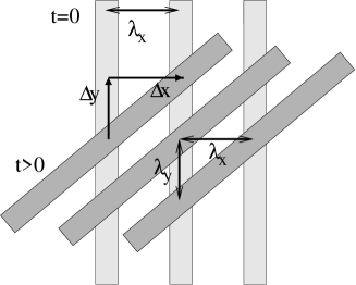
Figure 1: Advection by steady shear of a fluctuation in $x$-direction with wavelength $\lambda_{x}$ at $t=0$. At later time $t$, its wavelength $\lambda_{y}$ in $y$-direction obeys: $\lambda_{x}/\lambda_{y}=\Delta x/\Delta y=\dot{\gamma}t$.

Figure 1 sketches, neglecting Brownian motion, the advection of a fluctuation with initial wavevector $(2\pi/\lambda_{x},0,0)$, where $x$ points along the flow direction, into one with wavevector $(2\pi/\lambda_{x},2\pi/\lambda_{y}(t),0)$, where $\lambda_{y}(t)=\lambda_{x}/(\dot{\gamma}t)$ at later time $t$. Clearly, for any initial fluctuation with $\lambda_{x}\neq 0$, the wavelength in the gradient direction, $\lambda_{y}(t)$, will decrease for large times. Brownian particle motions (assisted by the interaction forces) “smear out” the fluctuation with time and cause the decay of the corresponding correlator. Because the advected wavelength decreases upon shearing, smaller and smaller motions can cause the fluctuation to decay. We presume that the shear advection of density fluctuations with wavevector $q_{p}$ leads to a competition between the non-linear feedback mechanism of the cage effect and the shear-induced decorrelation, and that this competition determines the nonlinear rheology of concentrated particle dispersions. Obviously, this competition involves a cooperative rearrangement of the (finite number of correlated) particles forming the distorted cage. Any microscopic theory like ours therefore requires severe uncontrolled approximations because no conceptually well-controlled approximation scheme appears suited to this problem. Thus, we build upon MCT (rather than, e.g., approaches starting with uncorrelated binary interactions, or based on coarse-graining procedures).

II.1 Structural dynamics under shear

We consider a suspension of $N$ Brownian particles, with density $n=N/V$, described by the Smoluchowski equation without hydrodynamic interactions. From time $t=0$ on, a flow is imposed in the solvent, which points in the $x$- and increases linearly along the $y$-direction: ${\bf v}({\bf r},t)=\mbox{\boldmath$\kappa$}\,{\bf r}\,\theta(t)=\dot{\gamma}\,y\,\hat{e}_{x}\,\theta(t)$ (where $\kappa$ is the shear rate tensor, $\kappa_{ij}=\dot{\gamma}\delta_{ix}\delta_{jy}$, and $\theta(t)$ the step function). Note that we neglect deviations from the imposed linear flow profile and thus cannot capture various shear-banding and other layering phenomena. (The latter may or may not arise in real experiments where only the stress, and not the velocity gradient, can be assumed constant across a sheared planar sample in steady state.) For this situation, the Smoluchowski equation for the particle distribution function is easily formulated Pusey85 ; russel ; dhont . But, with shear, its stationary solution is not known in general (except for some results at vanishing particle concentration Blawzdziewicz93 ; Bergenholtz01c ), and thus steady state quantities and correlation functions are not available.

Recently, Lionberger and Russel have made progress in the semidilute concentration regime by transferring liquid state approaches to the steady state situation; see Ref. Lionberger00 and works cited there. Yet, close to the glass transition where the quiescent system develops divergent time scales, a liquid state approach does not capture the falling out of equilibrium of the system, and thus (presumably) cannot handle the transition to dynamic yielding of a metastable solid. In order to capture the inherent long time scales we instead have suggested Fuchs02 to monitor the transient fluctuations of the suspension after turning on the solvent flow field at time $t=0$. Yet this problem too cannot be solved exactly, and requires approximations. First, the relevant variables whose transient dynamics shall be monitored, need to be chosen. Then equations of motion for these variables need to be formulated. To make progress we build upon the insights into the quiescent system provided by the MCT and generalize it to the out-of-equilibrium situation.

Colloidal suspensions upon densification exhibit a slowing down of the structural relaxation (particle rearrangements) and, to describe it, density fluctuations with wavevector ${\bf q}$ enter as natural variables, $\varrho_{\bf q}=\sum_{i=1}^{N}e^{i{\bf q}{\bf r}_{i}}$. Their magnitude is measured by the equilibrium structure factor $S_{q}=\langle\varrho^{*}_{\bf q}\varrho_{\bf q}\rangle/N$, which changes rather little, while their dynamics slows down dramatically. We follow MCT in considering the set of density fluctuations as a set of slow variables. Thus, arbitrary steady-state expectation values are obtained from determining the overlap of the relevant quantities with density fluctuations. This requires us to find the transient density fluctuations. They shall be determined from a closed set of equations of motion for the intermediate scattering functions, which is obtained by performing a mode coupling approximation.

With these approximations, various steady state quantities, like the thermodynamic shear stress Batchelor77 $\sigma=\langle\sigma_{xy}/V\rangle^{(\dot{\gamma})}$ can be calculated. (Note that steady state averages are abbreviated by $\langle\ldots\rangle^{(\dot{\gamma})}$, while equilibrium ones without shear are given by $\langle\ldots\rangle$.) The transverse stress also provides the shear viscosity which follows as $\eta(\dot{\gamma})=\eta_{\infty}+\sigma/\dot{\gamma}$, where the solvent viscosity is denoted $\eta_{\infty}$. Our final microscopic expression for the steady state stress $\sigma$ is found to be:

$$\sigma=\langle\sigma_{xy}/V\rangle^{(\dot{\gamma})}\approx\frac{k_{B}T\,\dot{\gamma}}{2}\int_{0}^{\infty}\!\!\!\!dt\,\int\!\!\frac{d^{3}k}{(2\pi)^{3}}\;\frac{k_{x}^{2}k_{y}k_{y}(t)}{k\,k(t)}\;\frac{S^{\prime}_{k}S^{\prime}_{k(t)}}{S^{2}_{k(t)}}\;\Phi^{2}_{{\bf k}}(t)\;,$$ (1)

with $t$ the time since switch-on, $k_{B}T$ the thermal energy, and $S^{\prime}_{k}=\partial S_{k}/\partial k$. The transient density fluctuations are given by $\Phi_{{\bf k}}(t)=\langle\varrho_{{\bf k}(t)}^{*}(t)\varrho_{\bf k}\rangle/(NS_{k})$ and are normalized by the quiescent $S_{k}$. Because of shear advection, time dependent wavevectors $k(t)=\sqrt{k^{2}+2k_{x}k_{y}\dot{\gamma}t+k_{x}^{2}\dot{\gamma}^{2}t^{2}}$ appear; a fluctuation with wavevector ${\bf k}$ at the start of shearing $t=0$ has a finite overlap with a fluctuation at the advected wavevector ${\bf k}(t)={\bf k}+{\bf k}\mbox{\boldmath$\kappa$}\,t$ at the later time $t>0$.

In summary, steady state quantities shall be determined by considering the structural relaxation under shearing and “integrating through the transient dynamics”. Because Pe${}_{0}\ll 1$, we expect ordering or layering transitions to be absent Laun92 ; and as hydrodynamic interactions are presumed to play a subordinate role during the structural relaxation Bergenholtz01b we neglect these too, focusing solely on the Brownian contribution to the transverse (shear) stress. A major approximation within our approach entails the elimination of explicit particle forces in favour of the quiescent-state structure factor $S_{q}$ (the only input in our theory and taken to be known). This is a near-equilibrium assumption that is formally uncontrolled but motivated, at least in part, by the smallness of Pe₀. Because we approximate nonlinear couplings under shear using equilibrium averages, we require the system to remain “close to equilibrium” in some sense. We leave to future work any attempt to make this sense more precise and, if possible, to relax the assumption involved.

II.2 Glass stability analysis

Little can be gained in our approach without specifying the dynamics of the transient intermediate scattering functions which describe how the equilibrium structure changes with time into that of a steadily sheared state. Obviously, any uncontrolled approximation (like mode coupling), which we are now forced to perform to obtain the equations of motion for the transient fluctuations, can introduce errors of unknown quality and magnitude into our results. But while the quantitative accuracy of the equations we propose in Ref.Fuchs02 has not been tested yet, there are qualitative conclusions which can be drawn from the structure of the equations, which are rather independent of the microscopic details of the approximation. Thus, in order to test our basic approach, these more universal aspects are of central interest and should be the ones chosen for initial comparison to experiments or simulations. We will consider only these aspects here, but in later sections two simple models are used to study how far the universal aspects dominate the model-dependent results.

The universal results which follow from our approach are connected to the stability equation of a (quiescently) arrested glassy structure which gets melted away by the imposed shear. From an expansion of the transient density fluctuations around the initially arrested structure close to the glass transition we get the bifurcation equations which describe how the localization driven by the cage effect competes with the fluidization induced by shearing. The derivation of a generalized “factorization theorem” and the so-called $\beta$-scaling equation, proceeds by a straightforward perturbation calculation which is given in Appendix A. Close to the bifurcation, the transient density fluctuations are given by one function ${\cal G}(t)$, which depends on control parameters, and determines the dynamics on all length scales:

$$\Phi_{q}(t)=f^{c}_{q}+h_{q}\,{\cal G}(t)\;.$$ (2)

The numbers $f_{q}^{c}$ describe the glassy structure at the instability and the critical amplitude $h_{q}$ is connected to the cage-breaking particle motion; both retain their definition from the unsheared situation. The function ${\cal G}(t)$ contains the essential non-linearities of the bifurcation dynamics which arise from the physical feedback mechanism (the cage effect) and the shear disturbance. It depends on a few material parameters only, and follows from

$$\varepsilon-c^{(\dot{\gamma})}\;(\dot{\gamma}\;t)^{2}+\lambda\;{\cal G}^{2}(t)=\frac{d}{dt}\;\int_{0}^{t}dt^{\prime}\;{\cal G}(t-t^{\prime})\;{\cal G}(t^{\prime})\;,$$ (3)

where $\varepsilon,\lambda$ and $c^{(\dot{\gamma})}$ are defined in Appendix A. The so-called separation parameter $\varepsilon$ measures the distance to the transition and the exponent parameter $\lambda$ determines power-law exponents resulting from Eq. (3), and is known for some systems Bengtzelius84 . The shear-related parameter $c^{(\dot{\gamma})}$ is a (relatively unimportant) number of order unity, which sets the scale for $\dot{\gamma}$ and could be absorbed into an effective shear rate $\sqrt{c^{(\dot{\gamma})}}\,\dot{\gamma}$.

The two derived equations, Eqs. (2,3), describe an expansion around the transition point between a non-Newtonian fluid and a yielding solid (within our approach, this applies whatever microscopic model is chosen) where divergent relaxation times arise from self-consistently calculated memory effects and compete with an externally imposed (shear-driven) loss of memory. Corrections of higher order in the small quantities ($\varepsilon,\dot{\gamma},{\cal G}$) are neglected in Eqs. (2,3); see Ref.Franosch97 for a calculation of the leading corrections and for background on Eq. (3) at $\dot{\gamma}=0$. In the following sections we will discuss two simplified models which, on the one hand, allow a more detailed analysis, and on the other hand share the universal stability properties derived from Eqs. (2,3).

III Models

We now present two, progressively more simplified, models that provide insights into the generic scenario of non-Newtonian flow, shear melting and solid yielding which emerge from our approach.

III.1 Isotropically sheared hard sphere model (ISHSM)

On the fully microscopic level of description of a sheared colloidal suspension, kinetic flow of the particles with the solvent leads to anisotropic dynamics. Yet, because of the strong hindering of the motion at high densities, which leads to a caging of particles, the development of the anisotropic “Taylor dispersion” may not yet be important at Pe $\simeq 1$ so that the motion stays locally isotropic. Recent simulation data of steady state structure factors support this consideration and indicate an isotropic distortion of the structure for Pe${}_{0}\ll 1$, while the Weissenberg number Pe is already large 1 Berthier02 . A mechanism which operates independently from Taylor dispersion arises from the shift of the advected wavevectors with time to higher values. As the effective potentials felt by density fluctuations evolve with increasing wavevector, this leads to a decrease of friction functions, speed-up of structural rearrangements and shear-fluidization. Therefore, one may hope that a model of isotropically sheared hard spheres (ISHSM), which for $\dot{\gamma}=0$ exhibits the nonlinear coupling of density correlators with wavelength equal to the average particle distance (viz. the “cage-effect”), and which, for $\dot{\gamma}\neq 0$, incorporates shear-advection, may be not too unrealistic.

Thus, in the ISHSM, the equation of motion for the density fluctuations at time $t$ after starting the shear is approximated by the one of the quiescent system:

$$\dot{\Phi}_{q}(t)+\Gamma_{q}\left\{\Phi_{q}(t)+\int_{0}^{t}\!\!\!dt^{\prime}\;m_{q}(t-t^{\prime})\,\dot{\Phi}_{q}(t^{\prime})\right\}=0\;.$$ (4)

where $\dot{\Phi}_{q}(t)=\partial_{t}\Phi_{q}(t)$, and the initial decay rate is $\Gamma_{q}=q^{2}D_{0}/S_{q}$ with the single particle Brownian diffusion coefficient given by the solvent viscosity, $D_{0}=k_{B}T/(3\pi\eta_{\infty}d)$. The memory function also is taken from the unsheared situation but now shear advection is entered into the overlap of the fluctuating forces with density fluctuations at time $t$:

$$m_{q}(t)\approx\frac{1}{2N}\sum_{{\bf k}}V^{(\dot{\gamma})}_{q,{\bf k}}(t)\;\Phi_{k}(t)\,\Phi_{|{\bf q}-{\bf k}|}(t)\;,$$ (5)

with

$$V^{(\dot{\gamma})}_{q,{\bf k}}(t)=\frac{n^{2}S_{q}S_{k}S_{p}}{q^{4}}\left[{\bf q}\cdot{\bf k}\;c_{k(t)}+{\bf q}\cdot{\bf p}\;c_{p(t)}\right]\left[{\bf q}\cdot{\bf k}\;c_{k}+{\bf q}\cdot{\bf p}\;c_{p}\right]$$ (6)

where ${\bf p}={\bf q}\!-\!{\bf k}$, and the length of the advected wavevector is approximated by $k(t)=k(1+(t\dot{\gamma})^{2}/3)^{1/2}$. The effective potentials are given by the direct correlation functions, $c_{q}=(1-1/S_{q})/n$. (For background on this model without shear, see Refs. Bengtzelius84 ; Goetze91b ; Franosch97 .)

For hard spheres, the quiescent $S_{q}$, taken from Percus-Yevick theoryrussel , depends only on the packing fraction $\phi$; discretising the wavevector integrations in Eq. (5) as done in Ref.Franosch97 , we find that the model’s glass transition lies at $\phi_{c}=0.51591$. Thus $\varepsilon$ (where $\varepsilon\simeq 3.0(\phi-\phi_{c})$), and $\dot{\gamma}$ are the only two control parameters determining the rheology. The exponent parameter becomes $\lambda=0.74$ and $c^{(\dot{\gamma})}\approx$ 3, while $S_{q}$ has its peak at $q_{p}=7/d$.

In the same spirit of incorporating advection as the only effect of shearing, the expression for the transverse modulus may be simplified to

$$\sigma=\frac{k_{B}T\,\dot{\gamma}}{60\pi^{2}}\;\int_{0}^{\infty}\!\!dt\;\int\!\!dk\;k^{4}\frac{S^{\prime}_{k}S^{\prime}_{k(t)}}{S^{2}_{k(t)}}\;\Phi_{k}^{2}(t)\;.$$ (7)

The resulting numerical results for the ISHSM are discussed below (section IV).

III.2 Schematic $F_{12}^{(\dot{\gamma})}$ model

The central features of the equations of motion of the ISHSM are that it reproduces the stability equation from the microscopic approach, Eq. (3), and that the vertex $V^{(\dot{\gamma})}$ contains the competition of two effects. First, it increases with increasing particle interactions (“collisions” or “cage effect”) which leads to a non-ergodicity transition in the absence of shear, and second, it vanishes with time because of shear-induced decorrelation. Both these effects can be captured in an even simpler “schematic” model, which moreover can be made to obey Eq. (3) also. This schematic F${}_{12}^{(\dot{\gamma})}$ model considers one normalized correlator $\Phi(t)$, with $\Phi(t\to 0)=1-\Gamma t\ldots$, which obeys a generalized relaxation equation:

$$\dot{\Phi}(t)+\Gamma\left\{\Phi(t)+\int_{0}^{t}\!\!\!dt^{\prime}\;m(t-t^{\prime})\,\dot{\Phi}(t^{\prime})\right\}=0\;.$$ (8)

Again, in the absence of the memory kernel $m$ the dynamics is trivial, $\Phi(t)=\exp({-\Gamma t})$, and a low order polynomial ansatz for $m$ suffices to study the generic schematic model. We choose

$$m(t)=\frac{1}{1+(\dot{\gamma}t)^{2}}\;\left(v_{1}\Phi(t)+v_{2}\Phi^{2}(t)\right)\;.$$ (9)

Without shear, this model has been studied extensively Goetze84 ; Goetze91b . Increasing particle caging is modeled by increasing coupling parameters $v_{1},v_{2}\geq 0$, and the only effect of shearing is to cause a time dependent decay of the friction kernel $m$. The system loses memory because of shearing. The role of the transport coefficient (viscosity) $\eta$ is played by the average relaxation time obtained from integrating the correlator, and this also is taken to determine the stress:

$$\sigma=\dot{\gamma}\;\eta=\dot{\gamma}\;\langle\tau\rangle=\dot{\gamma}\int_{0}^{\infty}\!\!\!dt\;\Phi(t)\;.$$ (10)

For the parameters of the model, values studied in the literature shall be taken. While the parameter $\Gamma$ just sets the time scale, the two interaction parameters are chosen as $v_{2}=v_{2}^{c}=2$ and $v_{1}=v_{1}^{c}+\delta v_{1}$, where $v_{1}^{c}=v_{2}^{c}(\sqrt{4/v_{2}^{c}}-1)\approx 0.828$. From an analysis similar to Appendix A, the critical non-ergodicity parameter is found as $f_{c}=1-\frac{1}{\sqrt{v_{2}^{c}}}\approx 0.293$ and the parameters in Eq. (3) emerge as follows:

$$\lambda=1-f_{c}\approx 0.707\;,\quad\varepsilon=\frac{\delta v_{1}f_{c}+\delta v_{2}f_{c}^{2}}{1-f_{c}}=\frac{\delta v_{1}f_{c}}{1-f_{c}}\;,\quad c^{(\dot{\gamma})}=\frac{v^{c}_{1}f_{c}+v^{c}_{2}f_{c}^{2}}{1-f_{c}}\approx 0.586\;.$$ (11)

The major advantage of this schematic model, besides its numerical simplicity, is that it encodes the two physical mechanisms at work in two handy parameters. The one, $\varepsilon$, parametrises the tendency of the undriven system to arrest, while the other, $\dot{\gamma}/\Gamma$, measures the loss of memory brought about by shearing.

IV Results and discussions

Both models described above exhibit a non-ergodicity transition which corresponds to an ideal fluid-to-glass transition within MCT. For $\dot{\gamma}=0$, upon smooth changes of the input equilibrium state parameters, a fluid with $\Phi_{q}(t\to\infty)\to 0$ turns into an amorphous solid, $\Phi_{q}(t\to\infty)\to f_{q}>0$. The $f_{q}$ are called glass form factors and describe the arrested structure. While transport coefficients of the fluid, like the viscosity, are connected to the longest relaxation time $\tau$ of the $\Phi_{q}(t)$, elastic constants of the solid, like the transverse elastic modulus $G_{\infty}$, are given by the $f_{q}$. (For some in-depth, albeit somewhat older, discussions of the idealized MCT see Refs. Goetze91b ; gs , and for a more recent discussion of experimental tests Ref. Goetze99 .)

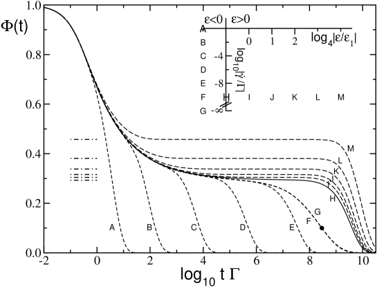
Figure 2: Correlators $\Phi(t)$ of the schematic $F_{12}^{(\dot{\gamma})}$ model for the separation parameters $\varepsilon$ and shear rates $\dot{\gamma}/\Gamma$ as marked in the inset; curves A to F for $\varepsilon=-\varepsilon_{1}=-10^{-3.79}$ and $\dot{\gamma}/\Gamma=10^{-n}$ with $n=0,2,\ldots,10$, while curve G corresponds to an unsheared fluid $\dot{\gamma}=0$ at $\varepsilon=-\varepsilon_{1}$ (a filled circle marks where the final relaxation time $\tau=10^{8.5}/\Gamma$ is read off, $\Phi(t=\tau)=0.1$). Curve H lies at the critical point $\varepsilon=0$ for $\dot{\gamma}/\Gamma=10^{-10}$, while I to M keep $\dot{\gamma}/\Gamma=10^{-10}$ but increase $\varepsilon=4^{n}\varepsilon_{1}$, $n=0,\ldots,4$. The horizontal bars indicate the heights of the non-ergodicity parameters $f$ for $\varepsilon\geq 0$ (compare curves H to M), which would be approached at long times for $\dot{\gamma}=0$, $\Phi(t\to\infty)=f$.

IV.1 Transient fluctuations

Figure 2 shows correlators of the $F_{12}^{(\dot{\gamma})}$ model for various shear-rates and distances from the non-ergodicity transition at $\varepsilon=0$. Curve G there corresponds to a non-sheared fluid state close to the transition, $\varepsilon=-\varepsilon_{1}=-10^{-3.79}$ and $\dot{\gamma}=0$. This shows the typical two-step relaxation pattern with microscopic short-time dynamics for $t\Gamma={\cal O}(1)$, followed by the approach to an intermediate plateau at $f_{c}\approx 0.293$, and the final decay characterised by the (final or $\alpha$-) relaxation time $\tau$. For positive separation parameters, $\varepsilon\geq 0$, the final decay is absent and the correlators approach finite long time limits $\Phi(t\to\infty)=f\geq f_{c}$ (not shown; these $f$’s are indicated by horizontal bars at the left of the figure). Including a finite shear rate corresponding to a small but finite bare Peclet number Pe${}_{0}=\dot{\gamma}/\Gamma$ in the model, little effect of shear on the short time dynamics is seen because of Pe${}_{0}\ll 1$. A drastic effect on the final decay, however, is seen in curves A to E, because the dressed Peclet (or Weissenberg) number Pe$=\dot{\gamma}\tau$ is not negligible. Moreover, all glassy curves ($\varepsilon\geq 0$), which would stay arrested for $\dot{\gamma}=0$, are seen to decay by a shear-induced process whose time scale is set by the inverse shear rate, and whose amplitude depends on the distance to the transition.

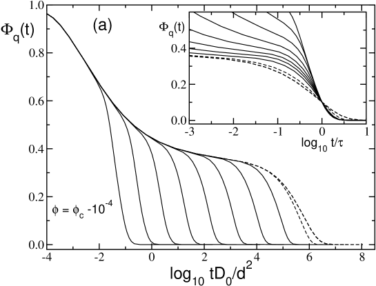
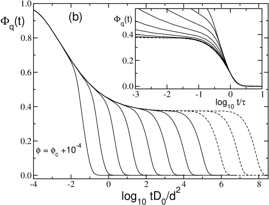
Figure 3: Normalized transient density correlators $\Phi_{q}(t)$ of the ISHSM at wavevector $q=3.4/d$ below (panel (a) at $\phi=\phi_{c}-10^{-4}$) and above (panel (b) at $\phi=\phi_{c}+10^{-4}$) the transition for increasing shear rates Pe${}_{0}=9^{n}*10^{-8}$ with $n=0,\ldots,10$ from right to left; the distances correspond to $\varepsilon=\pm 10^{-3.53}$. Curves for $n=$ 9, 10 carry short and for $n=$ 8 long dashes; note the collapse of the two short dashed curves in (a). The insets show the data rescaled so as to coincide at $\Phi(t=\tau)=0.1$.

The stability analysis of Eqs. (2,3) describes the correlators for a window around $\Phi_{q}\approx f_{q}^{c}$ and a finite window in time, which both can be estimated from the condition $|{\cal G}(t)|\ll 1$; for $\dot{\gamma}=0$ these have been worked out in detail Franosch97 . As the analysis in Appendix B shows, $(\dot{\gamma}t)^{2}$ dominates for long times in Eq. (3), and therefore always

$${\cal G}(t\to\infty)\to-t/\tau^{(\dot{\gamma})}\;,\quad\mbox{with }\quad\tau^{(\dot{\gamma})}=\sqrt{\frac{\lambda-1/2}{c^{(\dot{\gamma})}}}\;\frac{1}{|\dot{\gamma}|}\;.$$ (12)

Hence, under the imposed shear flow, density fluctuations always decay, as this decrease of ${\cal G}(t)$ for long times initiates the final relaxation of $\Phi_{{\bf q}}(t)$ to zero. (In this region the corrections to Eq. (2) of higher order in $\cal G$ become important.) Arbitrarily small steady shear rates $\dot{\gamma}$ melt the glass, as expected, and for small Pe₀ there appears a separation of time scales between short-time motion and the shear induced final decay; see curves H to M in figure 2.

For more detailed insight into the shapes of the relaxation curves, we turn to the ISHSM. Figure 3 displays density correlators at two densities, just below (panel (a)) and just above (panel (b)) the transition, for varying shear rates. Again, in almost all cases Pe₀ is negligibly small and the short-time dynamics is not affected. In the fluid case, the final or $\alpha$-relaxation is also not affected for the two smallest Pe values, but for larger Pe the non-exponential $\alpha$-relaxation becomes faster and less stretched; see the inset of fig. 3(a). (While the techniques of Appendix B allow us to discuss this shape change, we do not do so here for lack of space.) The glassy curves at $\varepsilon>0$, panel (b), exhibit a shift of the final relaxation with $\tau^{(\dot{\gamma})}$ and asymptotically approach a scaling function $\Phi_{q}^{+}(t/\tau^{(\dot{\gamma})})$. The master equation for the “yielding” scaling functions $\Phi_{q}^{+}$ in the ISHSM can be obtained from eliminating the short-time dynamics in Eq. (4). After a partial integration, the equation with $\dot{\Phi}_{q}(t)=0$ is solved by the scaling functions:

$$\Phi_{q}^{+}(\tilde{t})=m^{+}_{q}(\tilde{t})-\frac{d}{d\tilde{t}}\,\int_{0}^{\tilde{t}}d\tilde{t}^{\prime}\;m^{+}_{q}(\tilde{t}-\tilde{t}^{\prime})\Phi_{q}^{+}(\tilde{t}^{\prime})\;,$$ (13)

where $\tilde{t}=t/\tau^{(\dot{\gamma})}$, and the memory kernel is given by

$$m^{+}_{q}(\tilde{t})=\frac{1}{2N}\sum_{{\bf k}}V^{(\tilde{\dot{\gamma}})}_{q,{\bf k}}(\tilde{t})\;\Phi^{+}_{k}(\tilde{t})\,\Phi^{+}_{|{\bf q}-{\bf k}|}(\tilde{t})\;.$$ (14)

While the vertex is evaluated at fixed shear rate, $\tilde{\dot{\gamma}}=\sqrt{\frac{\lambda-\frac{1}{2}}{c^{(\dot{\gamma})}}}$, it depends on the equilibrium parameters. The corresponding results for the $F_{12}^{(\dot{\gamma})}$ can easily be obtained.

The importance of the $\beta$-correlator $\cal G$ for the derivation of the above scaling functions is because $\cal G$, according to Eq. (12), depends on $\tau^{(\dot{\gamma})}$ and not on internal time scales like $\tau$. It provides the initial conditions for Eq. (13), which follow from the analysis of Eq. (3) in Appendix B. In the glass, $\varepsilon>0$, Eq. (34) leads to

$$\Phi_{q}^{+}(\tilde{t}\to 0)=f^{c}_{q}+h_{q}\;\sqrt{\frac{\varepsilon}{1-\lambda}}\;\left[1-\frac{1-2\lambda}{4\varepsilon}\;\tilde{t}^{2}+{\cal O}(\frac{1}{\varepsilon^{2}}(\tilde{t})^{4})\right]\;,$$ (15)

and for somewhat longer times, $\tilde{t}\gg\sqrt{\varepsilon}$, according to Eq. (38), this merges into:

$$\Phi_{q}^{+}(\sqrt{\varepsilon}\ll\tilde{t}\ll 1)=f^{c}_{q}-h_{q}\;\tilde{t}\;.$$ (16)

At the transition, $\varepsilon=0$, Eq. (37) shows that Eq. (16) holds down to $\tilde{t}\to 0$. The scaling functions defined thereby describe the yielding behavior of a sheared glass where the relaxation time is set by the external shear rate and internal relaxation mechanisms are not active.

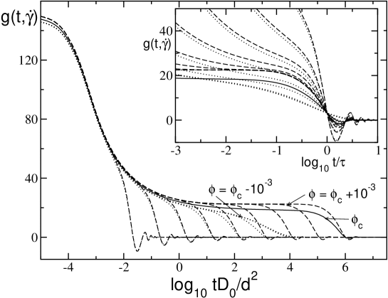
Figure 4: Transient non-Newtonian shear modulus $g(t,\dot{\gamma})$ of the ISHSM in units of $k_{B}T/d^{3}$ for the packing fractions $\phi=\phi_{c}\pm 10^{-3}$ ($\varepsilon=\pm 10^{-2.53}$; dashed/ dotted lines, respectively) for increasing shear rates Pe${}_{0}=9^{n}*10^{-6}$ with $n=0,\ldots,8$ from right to left; note the collapse of fluid lines for the smallest Pe₀. The solid line gives $g(t,\dot{\gamma})$ for $\phi=\phi_{c}$ and Pe${}_{0}=10^{-6}$. The inset shows the data rescaled so as to coincide at $g(t=\tau,\dot{\gamma})=5$; note the collapse of the $n=$ 6,7 & 8 curves for both $\phi>\phi_{c}$ and $\phi<\phi_{c}$.

Figure 4 shows the transient shear modulus $g(t,\dot{\gamma})$ of the ISHSM which determines the viscosity via $\eta=\int_{0}^{\infty}\!\!dt\,g(t,\dot{\gamma})$. It is the time derivative of the shear stress growth function $\eta^{+}(t,\dot{\gamma})$ (or transient start up viscosity; here, the ⁺ labels the shear historylarson ), $g(t,\dot{\gamma})=\frac{d}{dt}\eta^{+}(t,\dot{\gamma})$, and in the Newtonian-regime reduces to the time dependent shear modulus, $G(t)=g(t,\dot{\gamma}=0)$. The $g(t,\dot{\gamma})$ shows all the features exhibited by the correlator of the schematic model, and by the density correlators in the ISHSM, and thus the discussion based upon $\cal G$ and the yielding scaling law carries over to it. But in contrast to the correlator of the $F^{(\dot{\gamma})}_{12}$, and more so than the $\Phi_{q}$, the function $g(t,\dot{\gamma})$ becomes negative (oscillatory) in the final approach towards zero, an effect more marked at high Pe. This behavior originates in the general expression for $g(t,\dot{\gamma})$, Eq. (1), where the vertex reduces to a positive function (complete square) only in the absence of shear advection. A overshoot and oscillatory approach of the start up viscosity to the steady state value, $\eta^{+}(t\to\infty,\dot{\gamma})\to\eta(\dot{\gamma})$, therefore are generic features predicted from our approach.

In the discussion that follows, the leading corrections to the scaling law for the yielding correlators will be required. The analysis of Eq. (3) suggests that to next order for $\varepsilon\geq 0$:

$$\Phi_{q}(t)\to\Phi^{+}_{q}(\tilde{t})+\delta(\varepsilon,|\dot{\gamma}t_{0}|)\;\bar{\Phi}^{+}_{q}(\tilde{t})+{\cal O}(\delta^{2})\;,$$ (17)

where $t_{0}$ is a matching time, and the correction $\bar{\Phi}^{+}_{q}(\tilde{t})$ exhibits a weak divergence for short rescaled times, $\bar{\Phi}^{+}_{q}(\tilde{t}\to 0)\propto\tilde{t}^{-(2\lambda-1)/\lambda}$, as follows from Eqs. (37,38). The inset of fig. 3(b) shows the rise of the correlators above the yielding master function at short times and for very small Pe₀. Except for the fact that it is integrable, this function is of no further interest here. The small parameter $\delta$, however, sets the scale of the corrections and (as shown in Eqs. (37,38)) exhibits the following scaling properties

$$\delta\propto\left\{\begin{array}[]{lcl}|\dot{\gamma}t_{0}|^{m}&\mbox{ with }\,m=\frac{a}{1+a}\frac{2\lambda-1}{\lambda}&\mbox{for }\,\varepsilon=0\\ \varepsilon^{m^{\prime}}&\mbox{ with }\,m^{\prime}=\frac{2\lambda-1}{2\lambda}&\mbox{for }\,|\dot{\gamma}t_{0}|^{\frac{2a}{1+a}}\ll\varepsilon\ll 1\end{array}\right.$$ (18)

These results will be used below.

IV.2 Flow curves

In our approach, steady state properties of the sheared system are obtained via time integrals — from switching on the rheometer at $t=0$ up to very late times when the system has relaxed into the non-equilibrium stationary state. The evolution of the system is approximated by following the transient density fluctuations, which were discussed in the previous section for two specific simplified models. Equation (1) gives the thermodynamic shear stress in our fully microscopic approach, while Eqs. (7,10) give simplified expressions for it using the two models. Inserting the transient density correlators from section IV.1, the stress versus strain rate curves (“flow curves”) of the two models can be discussed. Such relations $\sigma(\dot{\gamma})$ often are postulated en route to deriving phenomenological “constitutive equations” for nonlinear flow behaviour, whereas our approach leads, in principle, to their microscopic derivation. Figures 5 to 8 present the results, the first two as plots of $\sigma$ versus $\dot{\gamma}$, while the second pair shows $\eta$ versus $\dot{\gamma}$. We will discuss the general qualitative features jointly for both models.

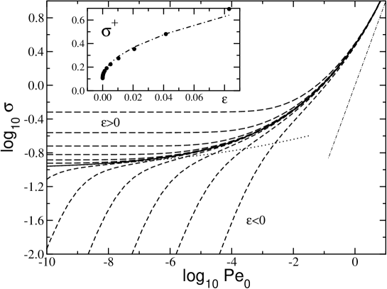
Figure 5: Steady state “stress” $\sigma=\dot{\gamma}\langle\tau\rangle$ in the schematic $F_{12}^{(\dot{\gamma})}$ model as function of Pe${}_{0}=\dot{\gamma}/\Gamma$ at various distances from the transition: $\varepsilon=0$ (solid line) and $\varepsilon=\pm 4^{n}\varepsilon_{1}$ for $n=-1,0,..,4$ (while $\varepsilon_{1}=10^{-3.79}$) with short (long) dashes for fluid $\varepsilon<0$ (glassy $\varepsilon>0$) curves. At $\varepsilon=0$, a dotted line gives $\sigma=\sigma^{+}_{c}(1+2.48\,\dot{\gamma}^{0.143})$ for $\dot{\gamma}\to 0$, with $\sigma_{c}^{+}=0.10$, while a thin dot-dashed line gives $\sigma_{c}=\dot{\gamma}$ for $\dot{\gamma}\to\infty$. The inset shows the finite limits $\sigma^{+}=\sigma(\varepsilon\geq 0,\gamma\to 0+)$ obtained above the transition; the dot-dashed curve is $\sigma^{+}=\sigma^{+}_{c}+1.88\sqrt{\varepsilon}$.

In the fluid, we find a linear or Newtonian regime in the limit $\dot{\gamma}\to 0$, where we recover the standard MCT approximations for the transport coefficients of a viscoelastic fluid Goetze91b ; gs . Hence $\sigma\to\dot{\gamma}\,\eta(\dot{\gamma}=0)$ holds for Pe $\ll 1$, as shown in figure 6, where Pe calculated with the structural relaxation time $\tau$ is included. As discussed in section II, the growth of $\tau$ (asymptotically) dominates all transport coefficients of the colloidal suspension and causes an proportional increase in the viscosity $\eta$. For Pe $>1$, the non-linear viscosity shear thins, and $\sigma$ increases sublinearly with $\dot{\gamma}$. Without analysing these complicated flow curves in detail here, we note that additional, shorter time scales than $\tau$ enter; these cause the shape change of the density correlators shown in figure 4(a) and also affect $\sigma$ and $\eta$. The stress versus strain rate figures 5, 6 clearly exhibit a broad crossover between the linear Newtonian and a much weaker (asymptotically) $\dot{\gamma}$-independent variation of the stress.

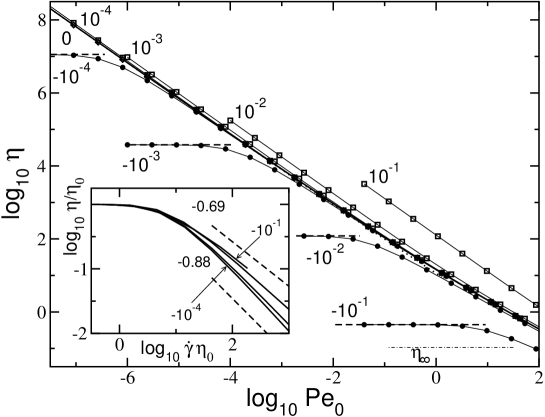
Figure 8: Steady state non-Newtonian shear viscosity $\eta$ in units of $k_{B}T/D_{0}d$ versus Pe${}_{0}=\dot{\gamma}d^{2}/D_{0}$, for the ISHSM at various distances from its glass transition, $\phi-\phi_{c}$ as labelled; data and line styles from figure 6 (the dot-dashed horizontal line gives the neglected background solvent viscosity). The inset shows the fluid curves $\varepsilon<0$ rescaled with the viscosity $\eta_{0}=\eta(\dot{\gamma}=0)$ of the quiescent fluid. Two power-laws (dashed lines) indicate the minimal and maximal slopes of the curves around $\dot{\gamma}\eta_{0}=10^{2}$.

Replotting the identical data as viscosity versus strain rate (figures 7, 8) these subtle features get compressed by the requirement of a much larger scale range on the viscosity axis; hence plotting stresses should prove more telling, close to a glass transition, than plotting viscosities. The latter can reveal subtle non-asymptotic corrections, but only if they are replotted on a smaller scale as done in the insets of figures 7, 8. There, various apparent power-law exponents could be fitted to the numerical data. Considering the ISHSM as a model for colloidal suspensions, the high-shear limiting viscosity contribution needs to be included; neglecting hydrodynamic interactions, this is set by the solvent viscosity $\eta_{\infty}$. The corresponding dot-dashed curves in figures 6, 8 show that a rather close approach to the critical packing fraction is required for the structural stress captured in Eq. (7) to dominate. Considering that hydrodynamic interactions cause an appreciable increase of the high-shear limiting viscosity over the solvent onerussel , this condition appears severe. However, it is obviously satisfied for systems that are nonergodic at rest ($\varepsilon>0$), if small enough $\dot{\gamma}$ can be achieved.

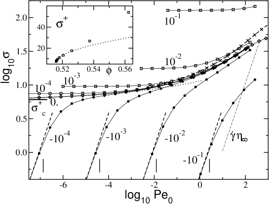
Figure 6: Steady state shear stress $\sigma$ in units of $k_{B}T/d^{3}$ versus Pe${}_{0}=\dot{\gamma}d^{2}/D_{0}$, for the ISHSM at various distances from its glass transition, $\phi-\phi_{c}$ as labeled; circles correspond to fluid, diamonds to the critical, and squares to glassy densities. For the fluid cases, $\phi<\phi_{c}$, dashed lines indicate Newtonian fluid behavior, $\sigma=\eta\dot{\gamma}$, while vertical bars mark Pe$=\dot{\gamma}\tau=1$, with the structural relaxation time taken from $\Phi_{q=7/d}(t=\tau)=0.1$. The stress which would additionally arise from the background solvent viscosity, $\sigma=\dot{\gamma}\eta_{\infty}$, is marked by a dot-dashed line. For the critical density, $\phi_{c}$, the critical yield stress, $\sigma^{+}_{c}=6.04$, is shown by a horizontal bar, and the dotted line $\sigma=\sigma^{+}_{c}(1+0.89\,\dot{\gamma}^{0.152})$ holds for $\dot{\gamma}\to 0$. Crosses connected by a thick dashed line give $\sigma$ at $\phi=\phi_{c}$ but for a different numerical discretization of the memory kernel (3-times larger cut-off $k_{\rm max}$). The inset shows the rise of the dynamical yield stress $\sigma^{+}=\sigma(\varepsilon\geq 0,\dot{\gamma}\to 0+)$ in the glass together with the fitted square root asymptote, $\sigma^{+}=\sigma_{c}^{+}+112\sqrt{\phi-\phi_{c}}$.

Above the transition, the quiescent system forms an (idealized) glassBengtzelius84 ; gs which exhibits finite elastic constants. The transverse elastic constant $G_{\infty}$ describes the (zero-frequency) Hookian response of the amorphous solid to a small applied shear strain $\gamma$, so that $\sigma=G_{\infty}\gamma$ for $\gamma\to 0$. If steady flow is imposed on the system, however, we find that the glass yields and is shear melted by arbitrarily small shear rates. This fluidization is not simply a trivial consequence of advection of the particles with the flow (Taylor dispersion is included in neither model) but implies that particles are freed from their cages and diffusion perpendicular to the shear plane also becomes possible. Hence, within our approach, infinitesimal steady shear leads to true melting of the glass and not merely plastic flow of it. Any finite shear rate, however small, sets a finite longest relaxation time, beyond which ergodicity is restored; see the discussion of figures 2, 3.

Nonetheless, a finite limiting stress (yield stress) must be overcome in order to maintain the flow of the glass: $\sigma(\dot{\gamma},\varepsilon>0)\to\sigma^{+}(\varepsilon)$ for $\dot{\gamma}\to 0$. To understand this better, note that for $\varepsilon\geq 0$ and $\dot{\gamma}\to 0$, the time $\tau^{(\dot{\gamma})}$ for the final decay , Eq. (12), can become arbitrarily slow compared to the time characterizing the decay onto $f_{q}$. Inserting the scaling functions $\Phi^{+}$ from Eqs. (13) to (16) into the expressions Eqs. (7,10) for the stress, the long time contributions separate out. Importantly, the integrands containing the $\Phi^{+}$ functions depend on time only via $\dot{\gamma}t$, so that nontrivial limits for the stationary stress follow in the limit $\dot{\gamma}\to 0$. In the ISHSM for $\varepsilon\geq 0$, this is given by (for $\dot{\gamma}>0$):

$$\sigma^{+}=\frac{k_{B}T\,\tilde{\dot{\gamma}}}{60\pi^{2}}\;\int_{0}^{\infty}\!\!d\tilde{t}\,\int\!\!dk\;k^{4}\;\frac{S^{\prime}_{k}S^{\prime}_{\tilde{k}(\tilde{t})}}{S^{2}_{\tilde{k}(\tilde{t})}}\;\left(\Phi^{+}_{k}(\tilde{t})\right)^{2}\;,$$ (19)

where $\tilde{k}(\tilde{t})=k\left(1+(\tilde{\dot{\gamma}}\tilde{t})^{2}/3\right)^{1/2}$, and the fixed reduced shear rate $\tilde{\dot{\gamma}}$ was defined after Eq. (14). The corresponding result in the $F^{(\dot{\gamma})}_{12}$ model is simply $\sigma^{+}=\tilde{\dot{\gamma}}\;\int_{0}^{\infty}\!d\tilde{t}\;\Phi^{+}(\tilde{t})$.

The existence of a dynamic yield stress in the glass phase is thus seen to arise from the scaling law in Eqs. (13,14), whose decay is initiated by the shear-induced asymptote of the correlator $\cal G$ in Eq. (12). Both the ISHSM and the schematic model share this feature. The yield stress arises from those fluctuations which require the presence of shearing to avoid their arrest. Importantly, even though $\sigma^{+}$ requires the solution of dynamical equations, within our approach it is solely and uniquely determined by the equilibrium structure factor $S_{q}$ at the transition point. Assuming the connections of MCT to the potential energy paradigm for glasses, as recently discussed Angelani00 ; Broderix00 , one might argue that $\sigma^{+}$ arises because the external driving allows the system to overcome energy barriers so that different metastable states can be reached. This interpretation would agree with the recent spin-glassBerthier00 and soft-glassy rheologySollich97 ; Sollich98b ; Fielding00 approaches. Our microscopic approach indicates how shear achieves this in the case of colloidal suspensions. It pushes fluctuations to shorter wavelengths where smaller particle rearrangements cause their decay.

The increase of the amplitude of the yielding master functions $\Phi^{+}$, see Eq. (15) originates in the increase of the arrested structure in the unsheared glass (via the non-ergodicity parameters $f_{q}-f_{q}^{c}\propto\sqrt{\varepsilon}$). In consequence the yield stress should rapidly increase as one moves further into the glass phase $\sigma^{+}-\sigma^{+}_{c}\propto\sqrt{\varepsilon}$ should (approximately) hold. Indeed, the insets of figures 6, 7 show a good fit of this square root increase to the numerical data. Our ability to make such a prediction is highly significant: the yield stress is an important non-linear property of the arrested state itself; it can be calculated here, because the yield stress is governed by the onset of melting under shear, which is itself a glass transition — not at $\phi\to\phi_{c}$ but at $\dot{\gamma}\to 0+$.

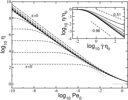
Figure 7: Shear dependent “viscosity” $\eta=\langle\tau\rangle$ (in units of $1/\Gamma$) in the schematic $F_{12}^{(\dot{\gamma})}$ model as function of Pe${}_{0}=\dot{\gamma}/\Gamma$ at various distances from the transition (data and line styles as in figure 5). The inset shows the fluid curves $\varepsilon<0$ rescaled with the viscosity $\eta_{0}=\eta(\dot{\gamma}=0)$ of the unsheared situation. Two power-laws (dashed lines) indicate the minimal and maximal slopes of the curves around $\dot{\gamma}\eta_{0}=10^{2}$.

An intriguing power-law increase of the stress above the yield value at the critical point was noticed in Ref.Fuchs02 and is also included (as dotted lines) in figures 5 and 6. It results from the leading corrections to the yielding scaling law summarized in Eqs. (17,18). Inserting those expressions into the integrals for the stress leads to the small shear rate expansion

$$\sigma=\sigma^{+}+|\dot{\gamma}t_{0}|^{m}\;\bar{\sigma}+{\cal O}(|\dot{\gamma}t_{0}|^{2m})\;,\quad\mbox{for }\;|\varepsilon|\ll|\dot{\gamma}t_{0}|^{\frac{2a}{1+a}}\;,$$ (20)

where the constant $\bar{\sigma}$ is given by an identical integral to that in Eq. (19) but with $\Phi^{+}$ replaced with the correction $\bar{\Phi}^{+}$. For the ISHSM the exponent $m$ turns out as $m=0.152$ while it is $m=0.143$ for the $F^{(\dot{\gamma})}_{12}$ model. As this prediction is based on the universal stability equation of a yielding glass, Eqs. (2,3), and on the existence of the yielding scaling law, Eqs. (13,14), our approach suggest that this Hershel-Bulkeleylarson flow curve may hold universally at a glass transition point, with the exponent $m$ depending on the material via the static structure factor $S_{q}$.

Another prediction from our asymptotic analysis of the leading corrections is borne out in the numerical calculations. Deep in the glass, Eqs. (17,18) and (20) state that the leading correction to $\sigma$ is independent on the shear rate $\dot{\gamma}$: $\sigma=\sigma^{+}+\varepsilon^{m^{\prime}}+{\cal O}(\varepsilon^{2m^{\prime}})$. This explains why in figures 5 and 6 the stress starts to rise with $\dot{\gamma}$ appreciably only when Pe₀ becomes non-negligible.

For the ISHSM, a caveat concerning the numerical results is required for shear rates beyond about Pe${}_{0}>10^{-2}$. The wavevector integrals in Eq. (5) do not converge properly for large $k$, and the results thus depend on the chosen cutoff, $k_{\rm max}=39.8/d$. This is implied by the crosses included in figure 6, which were calculated for $\phi=\phi_{c}$ but larger cutoff, $k_{\rm max}=119.8/d$. While only small differences (between the crosses and diamonds) remain for Pe${}_{0}<10^{-2}$, for larger shear rates the more accurate integrals lead to larger stresses. While this could be an artefact of the ISHSM, figure 5 shows that the time-dependent non-linear shear modulus $g(t,\dot{\gamma})$ decays rapidly for such large Peclet numbers. Because its initial value, $g(t=0,\dot{\gamma})$, is the instantaneous modulus of the unsheared system, $g(t=0,\dot{\gamma})=G(t=0)=\langle\sigma_{xy}^{2}\rangle/V$, this depends strongly on the particle interaction potential, and, for hard spheres should actually divergeLionberger94 ; Naegele98 . As changing $k_{\rm max}$ strongly influences $G(t=0)$, we presume that finite $k_{\rm max}$ effectively softens the particle repulsion. Only calculations for more general potentials can show whether this indicates a strong dependence of the non-linear stress on the steepness of the potential for not very small Peclet numbers. Interestingly, the glassy yield stress does not exhibit this strong dependence. It should however be noted that the ISHSM underestimates the effects of shearing as the ratio $\sigma^{+}_{c}/G^{c}_{\infty}=0.33$, is overestimated russel ; larson ; Nommensen99 .

IV.3 Structural versus non-structural features

Recently, computer simulations of sheared atomic glass formersYamamoto98 ; Barrat01 ; Berthier02 have been performed. While our microscopic theory is firmly based on assuming colloidal dynamics, in the simplified models, the effects of a different short time dynamics can easily be studied. Without shear, the MCT has found that the long-time structural relaxation is independent of the microscopic short time dynamicsFranosch98 ; Fuchs99 . (The latter only sets the overall time scale via the matching time $t_{0}$.) In the F${}_{12}^{(\dot{\gamma})}$ model, in order to mimic Newtonian dynamics, Eq. (8) can be replaced by

$$\ddot{\Phi}(t)+\nu\;\dot{\Phi}(t)+\Omega^{2}\,\left\{\Phi(t)+\int_{0}^{t}\!\!\!dt^{\prime}\;m(t-t^{\prime})\,\dot{\Phi}(t^{\prime})\right\}=0\;,$$ (21)

while Eq. (9) remains. Here, $\Omega$ is a microscopic vibrational frequency and $\nu$ a bare damping coefficient. Varying $\nu/\Omega$ shifts $t_{0}$, and the thin lines in figure 9 show the effect on the stress of the critical glassy state. The factor $x=(t_{0}^{\rm ND}\Omega)/(t_{0}^{\rm BD}\Gamma)$ varies between 0.3 and 5. As discussed in the context of the yielding scaling law, Eqs. (13,14) and Eq. (19), the yield stress $\sigma^{+}$ is, according to our approach, a purely structural property which is independent of the microscopic transient dynamics. Beyond the limit $\dot{\gamma}\to 0$, the one microscopic matching time $t_{0}$ enters the structural dynamics and affects the rise of $\sigma$. The data can be collapsed over a substantial window by replotting them versus $\dot{\gamma}t_{0}$ as explained by Eq. (20); see the bold lines in figure 9. This suggests that the expansion Eq. (20) could be extended to higher orders and might then obtain a larger range of validity. As the average relaxation time $\tau_{0}=\langle\tau(\dot{\gamma}=0)\rangle$ of an unsheared fluid state close to the transition is proportional to $t_{0}$, replotting the rescaled relaxation times (“viscosities”), $\langle\tau(\dot{\gamma})\rangle/\tau_{0}$, versus rescaled shear rate, $\dot{\gamma}\tau_{0}$, eliminates the $t_{0}$ dependence and leads to data collapse even though the the expected asymptotic power law, $\eta\propto\dot{\gamma}^{-1}$ is still strongly distorted.

To conclude, as argued already in section IV.2, even under shearing the structural relaxation remains independent of short time microscopic effects, except for shifts in the matching time $t_{0}$. According to this, simulations with either Newtonian or Brownian dynamics (that are otherwise identical) should thus observe the same nonlinear rheology near the glass transition. Rescaling with $t_{0}$ eliminates transient features and the nonlinear stress is only determined by the static structure factor for Pe${}_{0}\ll 1$. This last statement bears an important caveat though. The time $t_{0}$ is rather fast and thus not well separated from other microscopic time scales, so that corrections from finite Pe₀ need to be anticipated. This remains a task for future work.

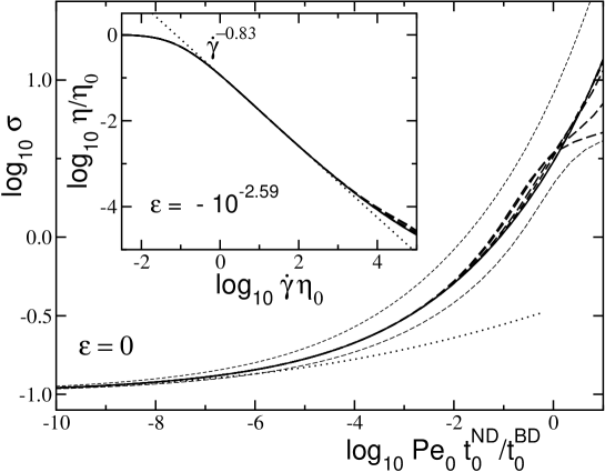
Figure 9: In the main panel, steady state “stress”, $\sigma=\dot{\gamma}\langle\tau\rangle$, versus rescaled Pe₀ for the schematic $F_{12}^{(\dot{\gamma})}$ model with different short time dynamics at the critical point $\varepsilon=0$; a dotted curve gives the Hershel-Bulkeley law from figure 5. In the inset, shear rate dependent “viscosity”, $\eta=\langle\tau\rangle$, for different short time dynamics below the transition, $\varepsilon=-4^{2}\varepsilon_{1}=-10^{-2.59}$, rescaled with the shear rate independent $\eta_{0}=\eta(\dot{\gamma}=0)$; a dotted lines gives a power-law fit. The viscosities $\eta_{0}$ at this $\varepsilon$ also determine the rescaling factors used in the main panel: $t^{\rm BD}_{0}/t^{\rm ND}_{0}=\eta^{\rm BD}_{0}/\eta^{\rm ND}_{0}$. Solid lines give Brownian dynamics results, while dashed curves correspond to Newtonian dynamics with $\nu/\Omega=5$, 1 (both short), 0.5, 0.1 and 0.01 (all three long dashes). Thin lines in the main panel give the unshifted $\sigma$ for $\nu/\Omega=5$ and 0.01.

IV.4 Non-linear Maxwell model

In 1863, Maxwell suggested a simple model for the linear rheological properties of a viscoelastic fluid, which has been the cornerstone of the phenomenology of glassy systems since then. He suggested that the time dependent shear modulus decays exponentially, $G(t)=G_{\infty}\,\exp{-t/\tau}$, where $G_{\infty}$ is the solid shear modulus and $\tau$ the structural relaxation time. Viscosity and stress follow as usual, $\sigma=\eta\dot{\gamma}=\dot{\gamma}\int_{0}^{\infty}\!\!dt\;G(t)$. Our results suggest, as a toy model, a non-linear extension of Maxwell’s model which captures the competition of structural arrest and shear-induced motion. It is obtained simply by postulating that the transient shear modulus can relax via two independent processes, an internal one characterized by $\tau$, and an induced or driven one characterized by $\tau^{(\dot{\gamma})}=c_{*}/|\dot{\gamma}|$ (with $c_{*}$ some numerical constant):

$$g^{\rm n-lM}(t,\dot{\gamma})=G_{\infty}\;e^{-t/\tau^{\rm M}}\;,\qquad\mbox{with }\;\frac{1}{\tau^{\rm M}}=\frac{1}{\tau}+\frac{1}{\tau^{(\dot{\gamma})}}\;.$$ (22)

From this the expression for the flow curve follows immediately as

$$\sigma=\dot{\gamma}\;\left[\eta_{\infty}+\frac{G_{\infty}\tau}{1+|\dot{\gamma}|\tau/c_{*}}\right]\;,$$ (23)

which exhibits a simplified scenario of the yielding-to flow transition which we derived within our microscopic approach; a glass would correspond to $1/\tau=0$, in which case the flow curve is that of a Bingham plastic. That toy model is not totally trivial, in that it gives a non-analytic dependence on the shear rate.

V Conclusions and outlook

Building on Ref.Fuchs02 , we have presented a microscopic theory of the nonlinear rheology of colloidal fluids and glasses under steady shear. This predicts a universal transition between shear-thinning fluid flow, with diverging viscosity upon increasing the interactions, and solid yielding, with a yield stress that is finite at (and beyond) the glass point. Numerical calculations presented here within progressively more simplified models support these universal predictions. The novel yielding behaviour is seen to arise from a competition between a collective caging of particles driven by increasing local order, and shear advection of the involved density fluctuations to smaller wavelengths, where Brownian particle motion relaxes them more effectively.

The shear-melting scenario can be rationalized solely from the stability analysis of a yielding solid summarized by Eqs. (2,3). As we tried to work out carefully, the properties of the correlator $\cal G$ and some (natural but as yet unproven, except for the models discussed here) assumptions about its extension to longer times suffice to explain our major predictions. These include: ($i$) The existence of a dynamic yield stress of glasses, which increases strongly with increasing density beyond the transition. ($ii$) The relatively small increase of the potential part of the stress in the solid above the yield value upon increasing $\dot{\gamma}$. ($iii$) The prediction of a Hershel-Bulkeley flow curve at the critical point, with a power law index fixed by the quiescent static structure factor. ($iv$) An asymptotic power-law shear thinning viscosity, $\eta\propto\dot{\gamma}^{-1}$ in the fluid (this follows from the existence of a yield stress). ($v$) The observation that motions for times shorter than the final relaxation time $\tau$ influence the stress or viscosity beyond Pe $=\dot{\gamma}\tau\ll 1$. This finding, discussed for a schematic model in section IV.3, predicts strong sub-leading corrections to points ($ii$)-($iv$) above and shows that more detailed calculations (which ought to include hydrodynamic interactions) are required, especially when no clear separation of time scales is present.

Reassuringly, the central non-linear stability equation, Eq. (3), which lies at the core of our predictions, can be argued on more general grounds than the explicit derivation we gave. Without shear, its predictions have been tested experimentally Megen93 ; Megen94b ; Goetze99 , and its structure thus appears established (with some confidence certainly for $\varepsilon<0$). The simplest inclusion of shear naturally leads to a term $-(\dot{\gamma}t)^{2}$ as the essential perturbation for long times. (Obviously the sign of $\dot{\gamma}$ must not matter, and the term must be negative to induce relaxation.) Also, because Eq. (3) without shear is a scaling equation without inherent time-scale (viz. ${\cal G}(y*t,\dot{\gamma}=0)$ is a solution for any $y>0$ if it is for $y=1$), the shear-rate $\dot{\gamma}$ can only enter multiplied by time $t$ itself. Thus we expect Eq. (3) to hold within a wider context of non-ergodicity transitions and hope that the predictions ($i$) to ($v$) above may apply to a broader class of scenarios describing yielding of metastable solids and shear thinning of viscoelastic fluids.

On the other hand, the approach we have outlined cannot address the shear thickening behaviour that, for many colloidal materials, occurs at higher flow rates than those addressed here (but in some cases appears to preclude shear thinning altogether). It has been suggested Liu98 ; Head01 that this jamming phenomenon is connected with a stress-induced glass transition. This avenue will be explored in future work on a version of the schematic model in which Eq. (9) is modified to include explicit stress- (as well as strain-rate-) dependence Holmes02 .

Appendix A Bifurcation analysis of the microscopic approach

To determine steady state quantities like the stress, the transient density fluctuations must be found within the suggested microscopic approximation scheme. With $t$ denoting the time after switching on the shear field, the normalized density correlators obey the exact equation of motion:

$$\dot{\Phi}_{\bf q}(t)+\Gamma_{\bf q}(t)\left\{\Phi_{\bf q}(t)+\int_{0}^{t}\!\!\!dt^{\prime}\;m_{\bf q}(t,t^{\prime})\,\dot{\Phi}_{\bf q}(t^{\prime})\right\}=0\;,$$ (24)

where the “initial decay rate” becomes time-dependent with shear and exhibits Taylor dispersion, $\Gamma_{\bf q}(t)\,S_{q}=D_{0}\left(q^{2}+q_{x}q_{y}\dot{\gamma}t+(q_{x}q_{y}\dot{\gamma}t+q_{x}^{2}\dot{\gamma}^{2}t^{2})S_{q}-(q_{x}q_{y}/q)\dot{\gamma}S^{\prime}_{q}\right)$. The memory function $m_{\bf q}(t,t^{\prime})$ can only be found after approximations, and, in the MCT spirit of our approach, is approximated by projecting the fluctuating forces onto density pairs and factorizing the resulting pair-density correlation functions:

$$m_{\bf q}(t,t^{\prime})\approx\frac{1}{2N}\sum_{{\bf k}}V^{(\dot{\gamma})}_{{\bf q},{\bf k}}(t,t^{\prime})\;\Phi_{{\bf k}}(t-t^{\prime})\,\Phi_{{\bf q}-{\bf k}}(t-t^{\prime})\;.$$ (25)

The vertex $V^{(\dot{\gamma})}$ is evaluated in the limit Pe${}_{0}\ll 1$ but for large times so that $\dot{\gamma}t$ and $\dot{\gamma}t^{\prime}$ are finite. As $\dot{\gamma}\to 0$, it reduces to the standard MCT vertex Bengtzelius84 and like the latter is uniquely determined by the equilibrium structure factor, $S_{q}$. For long times, it vanishes.

The (approximate) microscopic equations contain the central bifurcation singularity of MCT whose universal properties can be obtained from a stability analysis close to the singularity. It is these universal properties which the simplified models share. Around a quasi-arrested glassy structure, characterized by parameters $f^{c}_{q}$, the Eqs. (24,25) can be solved with the ansatz

$$\Phi_{{\bf q}}(t)=f^{c}_{q}+(1-f^{c}_{q})^{2}{\cal G}_{{\bf q}}(t)\;,$$ (26)

where we use the fact that without shear the system is isotropic and the (critical) glass form factor $f^{c}_{q}$ therefore depends on the magnitude $q$ only. Splitting the vertex close to the transition into its critical value and deviations,

$$V^{(\dot{\gamma})}_{{\bf q},{\bf k}}(t,t^{\prime})=V^{(0)c}_{{\bf q},{\bf k}}+\delta V^{(0)}_{{\bf q},{\bf k}}+\Delta V^{(\dot{\gamma})}_{{\bf q},{\bf k}}(t,t^{\prime})\;$$ (27)

the stability of $f^{c}_{q}$ can be determined. Introducing the (standard) abbreviations for time independent values, $m^{c}_{q}=\frac{1}{2N}\sum_{{\bf k}}V^{(0)c}_{{\bf q},{\bf k}}f^{c}_{k}f^{c}_{p}$ and $\varepsilon_{q}=\frac{1}{2N}\sum_{{\bf k}}\delta V^{(0)}_{{\bf q},{\bf k}}f^{c}_{k}f^{c}_{p}$, and for matrix coefficients in the expansion in $\cal G$, $C^{c}_{qk}=\frac{1}{N}\sum_{{\bf k^{\prime}}}V^{(0)c}_{{\bf q},{\bf k^{\prime}}}f^{c}_{k}(1-f^{c}_{p})^{2}\delta_{k,k^{\prime}}$ and $C^{c}_{qkp}=\frac{1}{2N}\sum_{{\bf k^{\prime}}}V^{(0)c}_{{\bf q},{\bf k^{\prime}}}(1-f^{c}_{k})^{2}(1-f^{c}_{p})^{2}\delta_{k,k^{\prime}}\delta_{p,|{\bf q}-{\bf k^{\prime}}|}$, Eq. (24) for long times becomes

$$\frac{f^{c}_{q}}{(1-f^{c}_{q})}-m^{c}_{q}+\left[{\cal G}_{q}(t)-\sum_{k}C^{c}_{qk}{\cal G}_{k}(t)\right]-$$

$$\varepsilon_{q}-\frac{1}{2N}\sum_{{\bf k}}\Delta V^{(\dot{\gamma})}_{{\bf q},{\bf k}}(t,0)\;f^{c}_{k}f^{c}_{p}-$$

$$\sum_{kp}C^{c}_{qkp}{\cal G}_{k}(t){\cal G}_{p}(t)+\frac{d}{dt}\sum_{k}C^{c}_{qk}(1-f^{c}_{q})\int_{0}^{t}\!\!dt^{\prime}\;{\cal G}_{k}(t-t^{\prime}){\cal G}_{q}(t^{\prime})+\ldots\;.$$ (28)

Here, a joint factor $(1-f^{c}_{q})$ was divided out and ($\ldots$) denotes both terms of higher order in $\cal G$ and those connected to the short time dynamics which become negligible for long times. For large enough vertices, the first two terms in Eq. (A) of order ${\cal G}^{0}$ have a finite solution $f^{c}_{q}$, which defines (idealized) glass points. A critical (glass) point, viz. bifurcation singularity in Eqs. (24,25), lies where the square bracket in Eq. (A) vanishes because $C^{c}_{qk}$ has eigenvalue 1, and the linearized equation cannot be solved for ${\cal G}(t)$, which gives the dynamics along the unstable direction, ${\cal G}_{q}(t)={\cal G}(t)e_{q}$. Here the eigenvectors of $C^{c}$ are denoted as $e_{q}$ and $\hat{e}_{q}$, which satisfy $\sum_{k}C^{c}_{qk}e_{k}=e_{q}$ and $\sum_{q}\hat{e}_{q}C^{c}_{qk}=\hat{e}_{k}$ and the (conveniently chosen) normalizations $\sum_{q}\hat{e}_{q}e_{q}=\sum_{q}\hat{e}_{q}(1-f^{c}_{q})e_{q}e_{q}=1$. The solvability equation for Eq. (A) results from requiring the contributions in the second and third lines to be perpendicular to $\hat{e}_{q}$, and without shear Eq. (3) follows upon the definitions: $\varepsilon=\sum_{q}\hat{e}_{q}\varepsilon_{q}$ and $\lambda=\sum_{qkp}\hat{e}_{q}C^{c}_{qkp}e_{k}e_{p}$; for more details see Goetze85 ; Goetze91b ; Franosch97 . With shear, a time dependent contribution arises from $\Delta V^{(\dot{\gamma})}_{{\bf q},{\bf k}}(t,0)$, and because of spatial isotropy in the limit of small shear, this reduces to:

$$t^{2}\;c^{(\dot{\gamma})}=\lim_{\dot{\gamma}\to 0}\frac{-1}{2N\dot{\gamma}^{2}}\;\sum_{{\bf q}{\bf k}}\;\hat{e}_{{\bf q}}\;\Delta V^{(\dot{\gamma})}_{{\bf q},{\bf k}}(t,0)\;f^{c}_{|{\bf k}|}\,f^{c}_{|{\bf q}-{\bf k}|}\;,$$ (29)

where $\hat{e}_{{\bf q}}=\frac{\hat{e}_{q}}{4\pi q^{2}V}$ takes care of three-dimensional integration. For colloidal hard spheres described with the Percus-Yevick structure factor russel , Monte Carlo integration estimates give $c^{(\dot{\gamma})}\approx 3$.

Appendix B Analysis of scaling equation (3)

The so-called $\beta$-correlator $\cal G$ is the solution of Eq. (3) with the prescribed short time behavior ${\cal G}(t\to 0)=(t_{0}/t)^{a}$ where $t_{0}$ is a matching time to the short time transient (determined by $\Gamma$), and the “critical” exponent $a$ obeys $\lambda=\Gamma^{2}(1-a)/\Gamma(1-2a)$. The derivation of this behaviour, which solves Eq. (A) at the singularity for long times, and the properties of $\cal G$ without shear can be found in Refs.Goetze85 ; Goetze91b ; Franosch97 . With shear, the analysis of Eq. (3) resembles the one of the extended MCT Fuchs92 , where a relaxation kernel describing thermally activated hopping motion lead to a term linear in $t$ instead of the quadratic $\dot{\gamma}^{2}t^{2}$. Because, in the main text, we focus on the yielding behavior of glassy solids, a discussion of the consequences of this quadratic term close to the glass transition and in the glass shall now be given for the regime where shear-induced motion dominates.

A useful aspect of ${\cal G}$ are its homogeneity properties. With $\Omega>0$ an arbitrary scale, it obeys

$${\cal G}(t,\varepsilon,\dot{\gamma})=\Omega^{a}\;\hat{\cal G}\left(\hat{t}=\Omega(t/t_{0}),\hat{\varepsilon}=\varepsilon\Omega^{-2a},\hat{\dot{\gamma}}=\dot{\gamma}t_{0}\Omega^{-(1+a)}\right)\;,$$ (30)

and thus does not change shape if the two control parameters are varied on a scaling line $\dot{\gamma}t_{0}=\hat{\dot{\gamma}}(\varepsilon/\hat{\varepsilon})^{(1+a)/(2a)}$. Moreover, this property enables one to define three regimes, $(i)$ $\varepsilon\ll-\varepsilon_{\dot{\gamma}}$ far below the transition in the fluid region, where finite shear barely distorts the fluid $\beta$-correlator; $(ii)$ $|\varepsilon|\ll\varepsilon_{\dot{\gamma}}$, in the transition region, where the dynamical anomalies are most pronounced; and $(iii)$ $\varepsilon\gg\varepsilon_{\dot{\gamma}}$ far above the transition in the shear yielding glassy state. Here, $\varepsilon_{\dot{\gamma}}=|\dot{\gamma}t_{0}|^{2a/(1+a)}$ defines a natural scale for the separation parameter $\varepsilon$, and throughout the following, $|\varepsilon|\ll 1$ and $\dot{\gamma}t_{0}\ll 1$ is assumed.

Equation (3) can then be solved by power series expansions with the general ansatz

$${\cal G}=t^{u}\;\sum_{n=0}\alpha_{n}t^{vn}\;,$$ (31)

which yields

$$\varepsilon-c^{(\dot{\gamma})}\;(\dot{\gamma}\;t)^{2}=\alpha_{0}^{2}\Gamma_{0,0}t^{2u}+2\alpha_{0}\alpha_{1}\Gamma_{0,1}t^{2u+v}+\sum_{n=2}t^{2u+nv}\sum_{n^{\prime}=0}^{n}\Gamma_{n-n^{\prime},n^{\prime}}\alpha_{n-n^{\prime}}\alpha_{n^{\prime}}\;.$$ (32)

Here, an abbreviation employing Gamma functions $\Gamma(x)$ is used:

$$\Gamma_{n,n^{\prime}}=\frac{\Gamma{(1+u+nv)}\Gamma{(1+u+n^{\prime}v)}}{\Gamma{(1+2u+(n+n^{\prime})v)}}-\lambda\;.$$ (33)

B.1 Glass for intermediate times

For any $\dot{\gamma}$, a solution to Eq. (32) can be found for $\varepsilon>0$ by choosing $u=0$. This requires $\alpha_{0}=\sqrt{\varepsilon/(1-\lambda)}$, $v=2$ and $\alpha_{1}=-c^{(\dot{\gamma})}\dot{\gamma}^{2}/(2\alpha_{0}(1-\lambda))$, while the higher coefficients can be found from a simple recursion relation. The result (with $\Omega=\varepsilon^{1/(2a)}$) takes the form

$${\cal G}(\varepsilon>0,t_{\rm f}\ll t\ll t_{b})=\sqrt{\varepsilon}\;\hat{\cal G}\left(\frac{t}{t_{0}}\varepsilon^{\frac{1}{2a}},+1,\dot{\gamma}t_{0}\varepsilon^{-\frac{1+a}{2a}}\right)=\sqrt{\varepsilon}\;\check{\cal G}(t/t_{b})=\sqrt{\frac{\varepsilon}{1-\lambda}}\;\left[1-\frac{c^{(\dot{\gamma})}}{2}(\frac{t}{t_{b}})^{2}+\ldots\right]\;,$$ (34)

where $t_{b}=\sqrt{\varepsilon}/|\dot{\gamma}|$ is a time scale that follows from balancing the first two terms in Eq. (3). Without shear, the correlator would adhere to $\sqrt{\varepsilon/(1-\lambda)}$ for long times in the glass, while for finite $\dot{\gamma}$ it relaxes below this value. The series Eq. (34) gives the solution of Eq. (3) for a finite window in time only, $t_{\rm f}\ll t\ll t_{b}$, as can be seen from its failure to match to the $(t_{0}/t)^{a}$ at short times, and as it has a finite radius of convergence of the order of $t_{b}$; the latter property can easily be determined from the recursion relation for the $\alpha_{n\geq 2}$. The obtained series thus describes, to order $\sqrt{\varepsilon}$, the initial stage of the final decay down from $f_{q}=f^{c}_{q}+\sqrt{\varepsilon/(1-\lambda)}$.

B.2 Transition region for long times

If, close to the transition, $\varepsilon=0$ can be set (region $(ii)$), then the choice $u=1$ requires $\alpha_{0}=\sqrt{c^{(\dot{\gamma})}/(\lambda-\frac{1}{2})}\;|\dot{\gamma}|$ in Eq. (32). To match the resulting long-time series, higher $\alpha_{n}$ are needed, and can be recursively be found, iff $\Gamma_{0,1}$ vanishes:

$$\Gamma_{0,1}=\frac{\Gamma{(2)}\Gamma{(2+v)}}{\Gamma{(3+v)}}-\lambda=0\qquad\Leftrightarrow v=-(2-\frac{1}{\lambda})\;.$$ (35)

Obviously, coefficient $\alpha_{1}$ then cannot be determined from Eq. (32), but needs to be found from matching to ${\cal G}$ at shorter times. Its scaling with $\dot{\gamma}$ can easily be obtained from the homogeneity statement, Eq. (30): $\alpha_{1}=\alpha_{0}\hat{\alpha}_{1}\,t_{\dot{\gamma}}^{-1/v}$, where $\hat{\alpha}_{1}$ is a matching constant (presumably of order unity), and the shear-rate dependent $\beta$-scaling time appears

$$t_{\dot{\gamma}}=t_{0}\;|\dot{\gamma}t_{0}|^{-\frac{1}{1+a}}\;.$$ (36)

As announced previously, the scaling function $\cal G$ then follows (with $\Omega=|\dot{\gamma}t_{0}|^{\frac{1}{1+a}}$):

$${\cal G}(\varepsilon=0,t\gg t_{\dot{\gamma}})=\sqrt{\varepsilon_{\dot{\gamma}}}\;\hat{\cal G}\left(\frac{t}{t_{\dot{\gamma}}},0,1\right)=|\dot{\gamma}t_{0}|^{\frac{a}{1+a}}\;\breve{\cal G}(t/t_{\dot{\gamma}})=-\sqrt{\frac{c^{(\dot{\gamma})}}{\lambda-\frac{1}{2}}}\;|\dot{\gamma}|t\;\left[1-\hat{\alpha}_{1}(\frac{t}{t_{\dot{\gamma}}})^{-\frac{2\lambda-1}{\lambda}}+\ldots\right]\;.$$ (37)

It matches to the decay of $\Phi(t)$ from unity down to $f^{c}$, which determines $\hat{\alpha}_{1}$, and describes the initial stage of the shear-induced decay of the correlators down from $f^{c}$ to zero.

B.3 Glass for long times

Deep in the glass, region $(iii)$, the same reasoning as in the case just studied can be used to determine $\alpha_{1}$ from matching — now to the series in Eq. (34). With $u=1$ and $v$ from Eq. (35), the scaling of the undetermined coefficient is fixed by requiring it to extend Eq. (34) from around $t_{b}$ to longer times: $\alpha_{1}=\alpha_{0}\hat{\alpha}^{\prime}_{1}\,t_{b}^{-1/v}$, where $\hat{\alpha}^{\prime}_{1}$ is another matching constant. The resulting series continues the shear induced decay of the correlators from the plateau value, as follows:

$${\cal G}(\varepsilon>0,t\gg t_{b})=|\dot{\gamma}t_{0}|^{\frac{a}{1+a}}\;\hat{\cal G}\left(\frac{t}{t_{\dot{\gamma}}},\frac{\varepsilon}{\varepsilon_{\dot{\gamma}}},1\right)=\sqrt{\varepsilon}\;\tilde{\cal G}(t/t_{b})=-\sqrt{\frac{c^{(\dot{\gamma})}}{\lambda-\frac{1}{2}}}\;|\dot{\gamma}|t\;\left[1-\hat{\alpha}^{\prime}_{1}(\frac{t}{t_{b}})^{-\frac{2\lambda-1}{\lambda}}+\ldots\right]\;.$$ (38)

References

- (1) R. G. Larson, The Structure and Rheology of Complex Fluids (Oxford University Press, New York, 1999).
- (2) W. B. Russel, D. A. Saville, and W. R. Schowalter, Colloidal Dispersions (Cambridge University Press, New York, 1989).
- (3) H. M. Laun, R. Bung, S. Hess, W. Loose, O. Hess, K. Hahn, E. Hädicke, R. Hingmann, F. Schmidt, and P. Lindner, J. Rheology 36, 743 (1992).
- (4) J. Bender and N. J. Wagner, J. Rheol. 40, 899 (1996).
- (5) P. Strating, Phys. Rev. E 59, 2175 (1999).
- (6) D. R. Foss and J. F. Brady, J. Fluid Mech 407, 167 (2000).
- (7) J. F. Brady, Cur. Opinion Colloid & Interf. Sci. 1, 472 (1996).
- (8) J. Bergenholtz, Cur. Opin. Coll. Interf. Sci. 6, 484 (2001).
- (9) G. Petekidis, P. N. Pusey, A. Moussaid, S. Egelhaaf, and W. C. K. Poon, Physica A 306, 334 (2002).
- (10) G. Petekidis, A. Moussaid, and P. N. Pusey, Phys. Rev. E ??, ?? (2002).
- (11) W. van Megen and P. N. Pusey, Phys. Rev. A 43, 5429 (1991).
- (12) W. van Megen and S. Underwood, Phys. Rev. Lett. 72, 1773 (1994).
- (13) C. Beck, W. Härtl, and R. Hempelmann, J. Chem. Phys. 111, 8209 (1999).
- (14) E. Bartsch, T. Eckert, C. Pies, and h. Sillescu, J. Non-Cryst. Solids ??, ?? (2002).
- (15) U. Bengtzelius, W. Götze, and A. Sjölander, J. Phys. C 17, 5915 (1984).
- (16) W. Götze, in Liquids, Freezing and Glass Transition, edited by J.-P. Hansen, D. Levesque, and J. Zinn-Justin (North-Holland, Amsterdam, 1991), p. 287.
- (17) W. Götze and L. Sjögren, Rep. Prog. Phys. 55, 241 (1992).
- (18) W. Götze, J. Phys.: Condens. Matter 11, A1 (1999).
- (19) M. Fuchs and M. E. Cates, cond-mat/0204628 (2002)
- (20) L. Berthier, J. L. Barrat, and J. Kurchan, Phys. Rev. E 61, 5464 (2000).
- (21) S. M. Fielding, P. Sollich, and M. E. Cates, J. Rheology 44, 323 (2000).
- (22) J. K. G. Dhont, An introduction to dynamics of colloids (Elsevier Science, Amsterdam, 1996).
- (23) J. Blawzdziewicz and G. Szamel, Phys. Rev. E 48, 4632 (1993).
- (24) J. Bergenholtz, J. F. Brady, and M. Vicic, J. Fluid Mech 456, 239 (2002).
- (25) R. A. Lionberger and W. B. Russel, Adv. Chem. Phys. 111, 399 (2000).
- (26) J. Bergenholtz and M. Fuchs, Phys. Rev. E 59, 5706 (1999).
- (27) W. van Megen, T. C. Mortensen, J. Müller, and S. R. Williams, Phys. Rev. E 58, 6073 (1998).
- (28) M. Fuchs, W. Götze, and M. R. Mayr, Phys. Rev. E 58, 3384 (1998).
- (29) L. Berthier and J. L. Barrat, cond-mat 0111312 (2001).
- (30) A. Onuki and K. Kawasaki, Ann. Phys. (N.Y.) 121, 456 (1979).
- (31) P. N. Pusey and R. J. A. Tough, in Dynamic Light Scattering: Application of Photon Correlation Spectroscopy, edited by R. Pecora (Plenum, New York, 1985), p. 85.
- (32) G. K. Batchelor, J. Fluid Mech 83, 97 (1977).
- (33) T. Franosch, M. Fuchs, W. Götze, M. R. Mayr, and A. P. Singh, Phys. Rev. E 55, 7153 (1997).
- (34) W. Götze, Z. Phys. B 56, 139 (1984).
- (35) L. Angelani, R. D. Leonardo, G. Ruocco, A. Scala, and F. Sciortino, Phys. Rev. Lett. 85, 5356 (2000).
- (36) K. Broderix, K. K. Bhattachrya, A. Cavagna, and Z. Zippelius, Phys. Rev. Lett. 85, 5360 (2000).
- (37) P. Sollich, F. Lequeux, P. Hebraud, and M. E. Cates, Phys. Rev. Lett. 78, 2020 (1997).
- (38) P. Sollich, Phys. Rev. E 58, 738 (1998).
- (39) R. A. Lionberger and W. B. Russel, J. Rheol 38, 1885 (1994).
- (40) G. Nägele and J. Bergenholtz, J. Chem. Phys. 108, 9893 (1998).
- (41) P. A. Nommensen, M. H. G. Duits, D. van den Ende, and J. Mellema, Phys. Rev. E 59, 3147 (1999).
- (42) R. Yamamoto and A. Onuki, Phys. Rev. E 58, 3515 (1998).
- (43) J. L. Barrat and L. Berthier, Phys. Rev. E 63, 012503 (2001).
- (44) T. Franosch, W. Götze, M. R. Mayr, and A. P. Singh, J. Non-Cryst. Solids 235–237, 71 (1998).
- (45) M. Fuchs and T. Voigtmann, Phil. Mag B 79, 1799 (1999).
- (46) W. van Megen and S. M. Underwood, Phys. Rev. Lett. 70, 2766 (1993).
- (47) W. van Megen and S. M. Underwood, Phys. Rev. E 49, 4206 (1994).
- (48) A. J. Liu and S. R. Nagel, Nature 396, 21 (1998).
- (49) D. A. Head, A. Ajdari, and M. E. Cates, Phys. Rev. E 64, 061509 (2001).
- (50) C. B. Holmes, M. Fuchs, and M. E. Cates, in preparation, (2002).
- (51) W. Götze, Z. Phys. B 60, 195 (1985).
- (52) M. Fuchs, W. Götze, S. Hildebrand, and A. Latz, J. Phys.: Condens. Matter 4, 7709 (1992).