Scaling properties of the projected $SO(5)$ model in three dimensions

Abstract

We study the scaling properties of the quantum “projected” $SO(5)$ model in three dimensions by means of a highly accurate Quantum-Monte-Carlo analysis. Within the parameter regime studied (temperature and system size), we show that the scaling behavior is consistent with a $SO(5)$-symmetric critical behavior in a relative extendent transient regime. This holds both when the symmetry breaking is caused by quantum fluctuations only as well as when also the static (mean-field) symmetry is moderately broken. We argue that possible departure away from the $SO(5)$ -symmetric scaling occurs only in an extremely narrow parameter regime, which is inaccessible both experimentally and numerically.

I Introduction

A common feature of the phase diagram of most high-T_c superconductors (HTSC) is the close proximity of the superconducting (SC) and the antiferromagnetic (AF) phases. The $SO(5)$ theory of high-T_c SC describes the transition between these two phases by an effective quantum non-linear $\sigma$ model with approximate $SO(5)$ symmetry, which unifies the two order parameters zhan.97 . Several microscopic $SO(5)$ -symmetric models have been proposed which succesfully describe many features of the cuprate physics ed.do.98 ; de.ko.98 ; hu.01 ; ar.be.97 ; so5.97 . A breakthrough has been recently achieved by a model that reconciles the $SO(5)$ symmetry with the physics of the Hubbard gap zh.hu.99 ; za.ha.00 . In the so-called “projected” $SO(5)$ (p$SO(5)$ ) model, the Gutzwiller projection is implemented exactly. Although the exact symmetry is destroyed at the microscopic level due to quantum fluctuations originating from the projection, it would be interesting to investigate whether an effective $SO(5)$ symmetry still controls the asymptotic behavior of the system at long-wavelength, i. e., $SO(5)$ symmetry is asymptotically restored. This has been shown to be the case, for example, for a two-leg ladder so5.97 system. This behavior is physically similar to the case of interacting Fermi liquids in which the characteristic symmetries of the non-interacting system – namely conservation of the particle number for each momentum $k$ of the Fermi surface – are destroyed by the interaction, but are asymptotically restored for low-energy excitations close to the Fermi surface. In contrast to the ladder, for a higher-dimensional system, the candidate for symmetry restoration should be sought at finite temperatures and is provided by the multicritical point where the AF and SC critical lines meet.

The problem of symmetry restoration at this multicritical point has been addressed by Hu in Ref. hu.01, via a Monte Carlo (MC) calculation of a classical $SO(5)$ model in which an additional quartic anisotropy term has been included. Classical MC are by orders of magnitude easier to perform and less resource demanding than QMC simulations, hence very large system sizes can be simulated and highly accurate data are obtained. For this reason Hu could carry out a detailed analysis of the AF-SC phase diagram and of the critical behavior. In particular, he could show that the SC helicity modulus follows a scaling law determined by the corresponding $SO(5)$ critical exponent $\nu_{5}$ and by the crossover exponent $\phi$. For these exponents, Hu could find a good agreement with the results of the $\epsilon$-expansion. On the other hand it was pointed out by Aharony ahar.02.comm via a rigorous argument that the decoupled fixed point is stable, and he further concluded that neither the biconical nor the $SO(5)$ fixed points are stable. However, he also commented that the unstable flow is extremely slow for the $SO(5)$ case due to the small crossover exponent.

In this paper, we address this issue by a detailed numerical analysis of the phase diagram and of the critical properties of the three-dimensional p$SO(5)$ model. Our strategy is, thus, to start from a model in which $SO(5)$ symmetry is realistically broken and to investigate to what extent this symmetry is restored at the multicritical point. Our main results are twofold. Within the system sizes and temperature ranges we can achieve, the scaling behavior is consistent with an $SO(5)$ critical behavior. On the other hand, since the $SO(5)$ fixed point could be ultimately unstable ahar.02.comm , we make an analytical estimate – based on the $\epsilon$-expansion – of the size of the critical region in which deviations from the $SO(5)$ behavior should be observed. Due to the small crossover exponent ahar.02.comm it turns out that the unstable flow only takes effect when the reduced temperature measured from the bi-critical point is very small. Therefore, the possible unstable effect can neither be observed experimentally nor numerically. For all practical purposes, the multicritical point is dominated by the initial flow towards the $SO(5)$-symmetric behaviormu.na.00 . Again, this situation is very similar to the case of Fermi liquids. Due to the well-known Kohn-Luttinger effect ko.lu.65 , the Fermi-liquid fixed point is always unstable towards a SC state. However, this effect is experimentally irrelevant for most metals since it only works at exponentially low temperatures.

II The model

In the p$SO(5)$ model each coarse-grained lattice site represents a plaquette of the original lattice model, and the lowest energy state on the plaquette is a spin singlet state at half-filling. There are four types of excitations, namely, three magnon modes and a hole-pair mode. Their dynamics are described by the following Hamiltonian:

$$\hat{H} = \Delta_{s}\!\!\!\!\!\sum_{x,\alpha{\scriptscriptstyle=2,3,4}}\!\!\!\!t_{\alpha}^{\dagger}{\scriptstyle(x)}t_{\alpha}{\scriptstyle(x)}+(\Delta_{c}\!-2\mu)\sum_{x}t_{h}^{\dagger}{\scriptstyle(x)}t_{h}{\scriptstyle(x)}$$

$$- J_{s}\!\!\!\!\!\!\!\!\!\!\sum_{<xx^{\prime}>,\alpha{\scriptscriptstyle=2,3,4}}\!\!\!\!\!\!\!\!n_{\alpha}{\scriptstyle(x)}n_{\alpha}{\scriptstyle(x^{\prime})}-\!J_{c}\!\!\!\sum_{<xx^{\prime}>}\!\!(t_{h}^{\dagger}{\scriptstyle(x)}t_{h}{\scriptstyle(x^{\prime})}\!+\!\mbox{h.c.})\,,$$

Here $t^{(\dagger)}_{\alpha=2,3,4}$ anihilates (creates) a triplet state, $t^{(\dagger)}_{h}$ anihilates (creates) a hole pair state and $n_{\alpha}=(t_{\alpha}+t^{\dagger}_{\alpha})/\sqrt{2}$ are the three components of the Néel order parameter. $\Delta_{s}$ and $\Delta_{c}\sim U$ are the energies to create a magnon and a hole-pair excitation, respectively, at vanishing chemical potential $\mu=0$. This model can also be effectively obtained by a coarse-grained reduction of more common models such as $t-J$ or Hubbard al.au.02 . In order to study the effect of symmetry breaking we consider different situations associated with different sets of parameters. First, we consider the case where $J_{s}=J=J_{c}/2$ (our zero of the chemical potential is such that $\Delta_{s}=\Delta_{c}$). It has been shown zh.hu.99 that this model has a static $SO(5)$ symmetry at the mean-field level and that the symmetry is only broken by quantum fluctuations ar.ha.00 . Since we want to carry out our analysis also for a more realistic model in which also the static $SO(5)$  symmetry is broken, we also consider a system with a different ratio $J_{s}/J_{c}$. In particular, one would like to reproduce the order of mangitude of $T_{c}/T_{N}$ observerved in the cuprates, where $T_{c}$ $(T_{N})$ denominates the SC critical temperature (Néel Temperature). However, this behavior is obtained for $J_{s}/J_{c}\sim 2$, for which the numerical simulation is rather unstable, making it impossible to determine the critical exponents with sufficient accuracy. For this reason, we choose a value of the parameter “in between” $(J_{c}=J_{h}=J)$, for which also the static $SO(5)$  symmetry is broken.

The phase diagram of this model in two dimensions has been analyzed in detail by a numerical Quantum-Monte-Carlo approach in Ref. do.ha.02 . In particular, the model has been shown to provide a semiquantitative description of many properties of the HTSC in a consistent way. In Ref. do.ha.02 , the SC transition has been identified as a Kosterlitz-Thouless phase in which the SC correlations decay algebraically. Unfortunately, there is no such transition for the AF phase in two dimensions, as all AF correlations decay exponentially at finite temperatures. Therefore, in order to analyze the multicritical point where the AF and SC critical lines meet, it is necessary to work in three dimensions, which is what we investigate in the present paper.

III Results

III.1 Case $J_{s}=J_{c}/2$

We start by presenting the phase diagram of the 3D p$SO(5)$ model for the “symmetric” case $J_{s}=J_{c}/2$. Figure 1 shows an AF and a SC phase extending to finite temperatures as expected. Furthermore, the two phase transition lines merge into a multicritical point (at $T_{b}\!=0.960\pm 0.005$ and $\mu_{b}\!=\!-0.098\pm 0.001$). The line of equal correlation decay of hole-pairs and triplet bosons also merges into this multicritical point $P$. Unlike the corresponding phase in the classical model, the SC phase extends only over a finite $\mu$ range; this is due to the hardcore constraint of the hole-pair bosons and agrees with experimentally determined phase diagrams of the cuprates. In this sense, the quantum mechanical p$SO(5)$ model is more physical than the classical $SO(5)$ model.

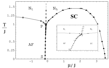
Figure 1: Phase diagram $T(\mu)$ of the three-dimensional p$SO(5)$ model with $J=J_{s}\!=\!J_{c}/2$ and $\Delta_{s}\!=\!\Delta_{c}\!=\!J$. N_h and N_t are, respectively, the hole-pair and the magnon-dominated regions of the disordered phase. The separation line between N_h and N_t is the line of equal spatial correlation decay of hole-pairs and bosons. The inset shows a detailed view of the region near the multicritical point.

However, in real cuprates the ratio between the maximum SC temperature $T_{c}$ and Néel temperature $T_{N}$ is about 0.17 to 0.25, whereas in the p$SO(5)$ model we obtain the values $T_{c}/J\!=\!1.465\pm 0.008$ at $\mu_{\mathit{opt}}/J\!\approx\!1.7$ and $T_{N}/J\!=1.29\pm 0.01$, hence $T_{c}$ is slightly larger than $T_{N}$. In order to obtain realistic values for the transition temperatures, it is necessary to relax the static $SO(5)$ condition and take a smaller value for the ratio $J_{c}/(2J_{s})$, which breaks $SO(5)$ symmetry even on a mean field level. The phase diagram with $J_{c}/(2J_{s})=0.225$ is plotted in Fig. 2. As one can see, this gives a more realistic ratio of $T_{N}/T_{c}\approx 0.2$. However, it should be pointed out that the numerical effort to treat such different values of $J$ is order of magnitudes larger than considering $J_{c}$ and $J_{s}$ of the same order of magnitude, as we have done in Fig. 1. Therefore, we will also consider a system with $J_{c}=J_{s}=1$ for which also the static $SO(5)$ symmetry is broken. For the same reason, we neglect here the $c$-axis anisotropy and consider an isotropic 3D model.

Figure 2: Phase diagram for $J_{c}/(2J_{s})=0.225$ as function of the hole doping $\delta$.

We first carry out an analysis of the critical properties for $J_{c}/(2J_{s})=1$ A closer look to the phase transition line between the points $S$ and $P$ reveals (inset of Fig. 1) that this line is not vertical as in the classical $SO(5)$ model but slightly inclined. This indicates that a finite latent heat is connected with the AF-SC phase transition. Moreover, this means that in contrast to the classical model, $\mu$ is not a scaling variable for the bicritical point $P$.

III.2 Scaling analysis

We now perform a scaling analysis similar to the one performed by Hu hu.01 in a classical $SO(5)$ system. The most important outcome of this analysis will be the strong numerical indication that in a large region around the multicritical point the full $SO(5)$ symmetry is approximately restored. This is non trivial for a system whose $SO(5)$ -symmetry has manifestly been broken by projecting out all doubly-occupied states. First we want to determine the form of the $T_{N}(\mu)$ and $T_{c}(\mu)$ curves in the vicinity of the bicritical point. For crossover behavior with an exponent $\phi>1$ one would generally expect that the two curves merge tangentially into the first-order line. However, this holds for the scaling variables, therefore, one should first perform a transformation from the old $\mu$ axis to a new $\mu^{\prime}$ axis defined by $\mu^{\prime}(T)=\mu-(T-T_{b})/m\,,$ where $m\approx 0.11$ is the slope of the first order line below $T_{b}$.

After this transformation, the transition curves $T_{N}(\mu^{\prime})$ and $T_{c}(\mu^{\prime})$ are quite well described by the crossover behavior (we now drop the prime for convenience)

$$\frac{T_{c}(\mu)}{T_{b}}-1=B_{2}\cdot(\mu-\mu_{b})^{1/\phi}$$

and $$\frac{T_{N}(\mu)}{T_{b}}-1=B_{3}\cdot(\mu_{b}-\mu)^{1/\phi}$$ (2)

The fit to this behavior is shown in more detail in Fig. 3. However, the value of $\phi$ we obtain ($\phi\approx 2.35$) is considerably larger than the value expected form the $\epsilon$-expansion. It should be noted that the above determination of $\phi$ is not very accurate: the data points in Fig. 3 are the result of a delicate finite-size scaling for lattice sites up to $18^{3}$, followed by the transformation from $\mu$ to $\mu^{\prime}$ which again increases the numerical error bars. For this reason it cannot be excluded that the difference in the $\phi$ values is mainly due to statistical and finite-size scaling errors. In fact, a more accurate evaluation of $\phi$ will be provided below.

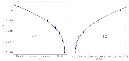
Figure 3: Plot of the AF (left) and SC (right) critical lines in the vicinity of the multicritical point.

On the SC side, the finite-size scaling carried out in order to extract the order parameter and the transition temperature turns out to be quite reliable. On the other hand, on the AF side, the fluctuations in the particle numbers of the three triplet bosons slightly increase the statistical errors of the SSE results and make the finite-size scaling more difficult.

The critical exponents for the onset of AF and SC order as a function of temperature for various chemical potentials can be extracted from Fig. 3. Far into the SC range, at $\mu\!=\!1.5$, we find for the SC helicity modulus fi.ba.73

$$\Upsilon\propto(1-T/T_{c})^{\nu}\quad\;\mbox{with}\quad\;\nu=0.66\pm 0.02\,,$$

which matches very well the values obtained by the $\epsilon$-expansion and by numerical analyses of a 3D XY model. On the AF side, error bars are larger, as discussed above. We obtain for the AF order parameter

$${C_{AF}(\infty)}\propto(1-T/T_{c})^{\beta_{3}}\quad\;\mbox{with}\quad\;\beta_{3}=0.35\pm 0.03,$$

for $\mu=-2.25$, also in accordance with the value expected for a 3D classical Heisenberg model.

In order to determine $\nu$ and $\phi$ more accurately in the crossover regime, we use two expressions derived from the scaling behavior (cf. Ref. hu.01 ).

$$\Upsilon(T_{b},\mu)/\Upsilon(T_{b},\mu^{\prime\prime})=\big{(}(\mu-\mu_{b})/(\mu^{\prime\prime}-\mu_{b})\big{)}^{\nu_{5}/\phi}\,.$$ (3)

and

$$\phi=\frac{\ln\Big{(}\frac{\mu_{2}-\mu_{b}}{\mu_{1}-\mu_{b}}\Big{)}}{\ln\bigg{(}\frac{\partial}{\partial T}\frac{\Upsilon(T,\mu_{1})}{\Upsilon(T,\mu_{1}^{\prime})}\Big{|}_{T=T_{b}}\Big{/}\frac{\partial}{\partial T}\frac{\Upsilon(T,\mu_{2})}{\Upsilon(T,\mu_{2}^{\prime})}\Big{|}_{T=T_{b}}\bigg{)}}\,$$ (4)

where $\mu_{1}$, $\mu_{1}^{\prime}$, $\mu_{2}$, and $\mu_{2}^{\prime}$ are related by $(\mu_{1}-\mu_{b})/(\mu_{1}^{\prime}-\mu_{b})\!=\!(\mu_{2}-\mu_{b})/(\mu_{2}^{\prime}-\mu_{b})>0$.

The result is shown in Fig. 4: we obtain the ratio

$$\nu_{5}/\phi=0.52\pm 0.01,$$

which is in excellent accordance with the results of the $\epsilon$-expansion and other numerical analyses hu.01 . $\phi$ is then obtained by using (4) . We have applied (4) onto 9 different combinations of $(\mu_{1},\mu_{1}^{\prime}\!=\!\mu_{2},\mu_{2}^{\prime})$ values with $\mu_{1}/\mu_{1}^{\prime}\!=\!\mu_{2}/\mu_{2}^{\prime}\!=\!0.5$. The result is

$$\phi=1.43\pm 0.05\,,$$

which is again in good agreement with the $\epsilon$-expansion for a $SO(5)$ bicritical point and with the results of Ref. hu.01 .

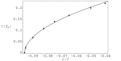
Figure 4: Helicity $\Upsilon$ as a function of the chemical potential $\mu$ at $T\!=\!T_{b}$. From this function, the value of $\nu_{5}/\phi$ can be extracted via equation (3).

III.3 Case $J_{s}=J_{c}$

This agreement between the critical exponents obtained in the previsous section may not come completely as a surprise, since the $SO(5)$ symmetry is only broken by quantum fluctuations for the parameter we have taken. The question we want to adress now is wether $SO(5)$ symmetry is also asymptotically restored for a more realistic set of parameters for which the static $SO(5)$ symmetry is broken as well. As already mentioned above, the case, where the phase diagram of the cuprates is qualitatively well reproduced ($J_{c}/(2J_{s})=0.225$, see Fig. 2), is too difficult to address numerically, so that the critical exponents cannot be determined with sufficient precision in this case. Therefore, we repeat our analysis for the model in an intermediate regime ($J_{c}=J_{h}$), which is not so realistic but for which the static $SO(5)$ symmetry is broken as well. One could hope that if $SO(5)$ symmetry is restored for here, then it might be also restored for the case $J_{c}/(2J_{s})=0.225$, although one may expect that the asymptotic region in which this occurs will be less extended. We stress again the fact that eventually one should expect the system to flow away from the $SO(5)$ fixed point, although in a very small critical region ahar.02.comm .

The phase diagram for $J_{c}=J_{h}$ is presented in Fig. 5 and a detailed view of the region close to the bicritical point is plotted in Fig. 6. Here, the points in the plots were obtained by a finite-size scaling with lattices up to 5032 $(18^{3})$ sites. In some cases, we were able to simulate lattices up to 10648 $(22^{3})$ sites. An example of the finite-size scaling is shown in Fig. 7. Our analysis yields $T_{b}=0.682\pm 0.005$ and $\mu_{b}=0.548\pm 0.0005$. Here the line of equal correlation decay is vertical within the error bars, so the transformation from $\mu$ to $\mu^{\prime}$ is not necessary and the error bars are not increased by the transformation. This allows to determine the critical exponents by fitting the data points visible in Fig. 6 against $T(\mu)=T_{b}*\left(1+(B_{2}+B_{3}*Sign[\mu_{b}-\mu])*\mid x-\mu_{b}\mid^{\frac{1}{\phi}}\right)$. We obtain:

$$B_{2} = 0.47\pm 0.07,$$ (5)

$$B_{3} = 0.11\pm 0.04,,$$ (6)

$$\phi = 1.49\pm 0.18,$$ (7)

$$Tb = 0.683\pm 0.004,$$ (8)

$$\frac{B_{2}}{B_{3}} = 1.67,\pm 0.36$$ (9)

Since points further away from the bicritical point are expected to show a larger deviation from the bicritical behavior, we also performed a weighted fit, which takes this fact into account. Here, data points closer to the bicritical point are weighted more than the ones further away. Specifically, in both the SC and the AF phase, the point closest to the bicritical point is weighted six times the one with the largest distance to the bicritical point. The second closest is weighted 5 times and so on. The results are, within the error bars, quite similiar to the ones obtained without this different weighting procedure:

$$B_{2} = 0.46\pm 0.05,$$ (10)

$$B_{3} = 0.11\pm 0.03,$$ (11)

$$\phi = 1.53\pm 0.12$$ (12)

$$Tb = 0.682\pm 0.003$$ (13)

$$\frac{B_{2}}{B_{3}} = 1.61\pm 0.23$$ (14)

The agreement between Eqs. 5-9 and Eqs. 11-14 suggests that the data we have considered are still controlled by the bicritical point,

In order to test whether alternativly proposed fixed points may be excluded, we carried out a least-square fit of our data to the decoupled fixpoint case ($\phi=1,B_{2},B_{3}$ and $T_{b}$ arbitrary). This is shown in Fig.  6 (dashed-dotted line). As one can see form the curve, our data doe not support the assumption that the p$SO(5)$ model has a decoupled fixpoint. Since we know that ultimately the decoupled fixed point should be the stable one ahar.02.comm , this means that our systems is still quite far away from the ultimate asymptotic region.

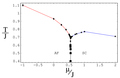
Figure 5: Phase diagram as a function of the chemical potential for $J_{c}=J_{h}=1$, the lines are guides to the eyes.

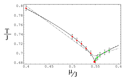
Figure 6: Detailed view of the phase diagram as a function $\mu$ ($J_{c}=J_{h}=1$), the two lines have been obtained by fits to $T(\mu)=T_{b}*\left(1+(B_{2}+B_{3}*Sign[\mu_{b}-\mu])*\mid\mu-\mu_{b}]^{\frac{1}{\phi}}\right)$. The continuous (dashed) line is the ‘normal’ (‘weighted’) fit. The decoupled fixpoint case is plotted as a dashed-dotted line.

Figure 7: Finite size scaling of the antiferromagnetic order parameter for $\mu=0.5$, the temperatures cover 0.72J (lozenge), 0.73J (star), 0.735 (square), 0.74J (triangle) and 0.75 (cirle). The lattice size was varied from 216 $(8^{3})$ upto 10648 $(22^{3})$ sites, scanning all cubes with even edge length.

IV Discussion and conclusions

Altogether, the scaling analysis of the 3D p$SO(5)$ model has produced a crossover exponent which matches quite well with the corresponding value obtained from a classical $SO(5)$ model and from the $\epsilon$-expansion. This gives convincing evidence that the static correlation functions at the p$SO(5)$ multicritical point is controlled by a fully $SO(5)$ symmetric point, at least in a large transient region. However, one should point out that within the statistical and finite-size error, as well as within the error due to the extrapolation of the $\epsilon$-expansion value to $\epsilon=1$ one cannot exclude that the actual fixed point one approaches is the biconical one, which has very similar exponents to the isotropic $SO(5)$ one. On the other hand, the biconical fixed point should be accompanied by a AF+SC coexistence region (as a function of chemical potential), which we do not observe. As discussed above we can certainly exclude in this transient region the decoupled fixed point for which $\phi=1$ahar.02.comm . Of course, our limited system sizes cannot tell which fixed point would be ultimately stable in the deep asymptotic region. Here, Aharony’s exact statement shows that the decoupled fixed point should be ultimately the stable one in the deep asymptotic region ahar.02.comm .

We argue that the resolution between this exact result and the numerically observed $SO(5)$ critical behavior lies in the size of the critical region ahar.02.comm . We now give an estimate, based on $\epsilon$ expansion, for the scale at which the instability of the $SO(5)$ fixed point could be detectable. This estimate holds for the case in which one has a “static” $SO(5)$ symmetry at the mean-field level. The symmetry-breaking effects due to quantum fluctuations have been estimated in Ref. ar.ha.00 and are given by Eq. (36) there. By replacing the initial conditions for the bare couplings in terms of the microscopic parameters of the Hamiltonian (cf. Eq. 26 of Ref.  ar.ha.00 ), and projecting along the different scaling variables around the $SO(5)$ fixed point, one obtains a quite small projection along the variable that scales away from the fixed point. Combined with the fact that the exponent for this scaling variables is quite small ($\lambda=1/13$ at the lowest-order in the $\epsilon$ expansion, although more accurate estimates ca.pe.02u ; ca.pe.03 ; pe.vi.02 give a somewhat larger value of $\lambda\approx 0.3$), we obtain an estimate for the scaling region in which the $SO(5)$ fixed point is replaced by another – e.g. the biconical or the decoupled – fixed point at $t\equiv(T_{b}-T)/T_{b}\sim 10^{-10}$ if one takes the $O(\epsilon)$ result for the exponent. Notice that taking the result of Ref. ca.pe.03 for the exponent, one obtains a quite larger value $t\sim 2.10^{-3}$. However, since the multi-critical temperatures of relevant materials (organic conductors, and, more recently, $YBa_{2}Cu_{3}O_{6.35}$) are around $10\ K$, the critical region is still basically unaccessible experimentally as well as with our quantum simulation. On the other hand, the other scaling variables, although being initially of the order of $1$, rapidly scale to zero due to the large, negative, exponents. Therefore, the $SO(5)$ regime starts to become important as soon as the AF and SC correlation lengths become large and continues to affect the scaling behavior of the system basically in the whole accessible region.

In conclusion, we have shown numerically that the p$SO(5)$ model, which combines the idea of $SO(5)$ symmetry with a realistic treatment of the Hubbard gap, reproduces the salient features of the cuprate’s phase diagram. Furthermore, this model is controlled by a $SO(5)$ symmetric bicritical point, at least within a large transient region. We have shown that this also holds for a case in which the static $SO(5)$ symmetry is broken. Possible flow away from the symmetric fix point occurs only within an extremely narrow region in reduced temperature, making it impossible to observe both experimentally and numerically. We would like to point out that this situation is very similar to many other examples in condensed-matter physics. The ubiquitous Fermi-liquid fix point is strictly speaking always unstable because of the Kohn-Luttinger effectko.lu.65 . But for most metals this instability occurs only at extremely low temperatures, and is practically irrelevant. Another example is the “ordinary” superconductor to normal-state transition at $T_{c}$. Strictly speaking, coupling to the fluctuating electromagnetic field renders this fix point unstableha.lu.74 . However, this effect has never been observed experimentally, since the associated critical region is too small. Therefore, irrespective of the question of ultimate stability, we argue that the $SO(5)$ fix point is a robust one in a similar sense, and it controls the physics near the AF and SC transitions.

References

- (1) S.-C. Zhang, Science 275, 1089 (1997).
- (2) R. Eder, A. Dorneich, M. G. Zacher, W. Hanke, and S.-C. Zhang, Phys. Rev. B 59, 561 (1999).
- (3) E. Demler, H. Kohno, and S.-C. Zhang, Phys. Rev. B 58, 5719 (1998).
- (4) X. Hu, Phys. Rev. Lett. 87, 057004 (2001).
- (5) D. P. Arovas, A. J. Berlinsky, C. Kallin, and S.-C. Zhang, Phys. Rev. Lett. 79, 2871 (1997).
- (6) E. Arrigoni and W. Hanke, Phys. Rev. Lett. 82, 2115 (1999).
- (7) S.-C. Zhang, J.-P. Hu, E. Arrigoni, W. Hanke, and A. Auerbach, Phys. Rev. B 60, 13070 (1999).
- (8) M. G. Zacher, W. Hanke, E. Arrigoni, and S.-C. Zhang, Phys. Rev. Lett. 85, 824 (2000).
- (9) A. Aharony, Phys. Rev. Lett. 88, 059703 (2002).
- (10) S. Murakami and N. Nagaosa, J. Phys. Soc. Jpn. 69, 2395 (2000).
- (11) W. Kohn and J. M. Luttinger, Phys. Rev. Lett. 15, 524 (1965).
- (12) E. Altman and A. Auerbach, Phys. Rev. B 65, 104508 (2002).
- (13) E. Arrigoni and W. Hanke, Phys. Rev. B 62, 11770 (2000).
- (14) A. Dorneich, W. Hanke, E. Arrigoni, M. Troyer, and S. C. Zhang, Phys. Rev. Lett. 88, 057003 (2002).
- (15) M. E. Fisher, M. N. Barber, and D. Jasnow, Phys. Rev. A 8, 1111 (1973).
- (16) P. Calabrese, A. Pelissetto, and E. Vicari, cond-mat/0203533 (unpublished).
- (17) P. Calabrese, A. Pelissetto, and E. Vicari, Phys. Rev. B 67, 054505 (2002).
- (18) A. Pelissetto and E. Vicari, Phys. Rep. 368, 549 (2000).
- (19) B. I. Halperin, T. C. Lubensky, and S.-K. Ma, Phys. Rev. Lett. 32, 292 (1974).