Thermodynamics of the half-filled Kondo lattice model around the atomic limit

Abstract

We present a perturbation theory for studying thermodynamic properties of the Kondo spin liquid phase of the half-filled Kondo lattice model. The grand partition function is derived to calculate chemical potential, spin and charge susceptibilities and specific heat. The treatment is applicable to the model with strong couplings in any dimensions (one, two and three dimensions). The chemical potential equals zero at any temperatures, satisfying the requirement of the particle-hole symmetry. Thermally activated behaviors of the spin(charge) susceptibility due to the spin(quasiparticle) gap can be seen and the two-peak structure of the specific heat is obtained. The same treatment to the periodic Anderson model around atomic limit is also briefly discussed.

The Kondo lattice model (KLM) and the periodic Anderson model (PAM) are two prototype models for the heavy fermion system and related materialslee ; fulde ; hewso . Both models describe a band of itinerant conduction electrons interacting with a lattice of magnetic impurities. At half-filling, they are usually viewed as standard models to understand the so-called Kondo insulator. The PAM is written as

$$H_{PAM} = -t\sum_{\langle i,j\rangle,s}(c^{{\dagger}}_{is}c_{js}+H.c.)+V\sum_{i,s}(c^{{\dagger}}_{is}f_{is}+H.c.)$$ (1)

$$+\epsilon_{f}\sum_{i}n^{f}_{i}+U_{f}\sum_{i}n^{f}_{i\uparrow}n^{f}_{i\downarrow},$$

where the fermion operators $c^{{\dagger}}_{is}$ ($f^{{\dagger}}_{is}$) create conduction (impurity) electrons and the summation $\sum_{\langle i,j\rangle}$ is taken over all nearest neighbors. In the Kondo limit, $U_{f}\gg V$ and $\epsilon_{F}\gg\epsilon_{f}$ ($\epsilon_{F}$ is the Fermi energy), the charge fluctuation of $f$ electrons is suppressed and each impurity site is occupied by one and only one $f$ electron. Then the PAM can be simplified and reduced to the KLMschr ,

$$H_{KLM}=-t\sum_{\langle i,j\rangle,s}(c^{{\dagger}}_{is}c_{js}+H.c.)+J\sum_{i}{\bf S}_{i}\cdot{\bf s}^{c}_{i},$$ (2)

with the spin-exchange coupling $J=8V^{2}/U_{f}$ under symmetric conditions. Here ${\bf s}^{c}=\sum_{s,s^{\prime}}\frac{1}{2}{\bf\sigma}_{s,s^{\prime}}c^{\dagger}_{is}c_{is^{\prime}}$ is the spin-density operator of conduction electrons and ${\bf S}=\sum_{s,s^{\prime}}\frac{1}{2}{\bf\sigma}_{s,s^{\prime}}f^{\dagger}_{is}f_{is^{\prime}}$ denotes the localized spin with $f^{\dagger}_{is}$ ($f_{is}$) being the pseudo-fermion operators. ${\bf\sigma}_{s,s^{\prime}}$ is the Pauli matrix.

The purpose of this work is mainly to consider the half-filled KLM whose ground state and finite-temperature properties have been intensively studied in recent yearstsun ; wang ; shi ; capp ; shib . The ground-state phase diagram has been now well establishedtsun . Owing to the Kondo screening effect, the one dimensional (1D) model has a Kondo spin liquid (KSL) state at all values of the coupling $J/t$. In higher dimensions, it is suggested that competition between the Kondo screening and the Ruderman-Kittel-Kasuya-Yosida interaction leads to quantum phase transitions from the KSL state to the antiferromagnetically ordered state as $J/t$ decreases, with the critical point $(J/t)_{c}\approx 1.4$ for two-dimensional (2D) and $2.0$ for three-dimensional (3D) KLM’swang ; shi ; capp . The KSL phase is characterized by three different energy scales: the spin ($\Delta_{s}$), charge ($\Delta_{c}$) and quasiparticle ($\Delta_{qp}$) gaps. The spin gap vanishes at the critical point while the other two gaps still remain finite in the ordered phase. The finite-temperature properties of the KSL phase are dominated by all three energy scales. A number of powerful numerical methods including quantum Monte Carlo (QMC) simulationscapp , the density matrix renormalization group methodshib and the finite-temperature Lanczos techniquehaule have been used to investigate the thermodynamic properties of the KLM in 1D and 2D. However, less analytical work is known, especially for the higher dimensional models.

In this paper, we propose a finite-temperature perturbation theory to study the thermodynamics of the KSL phase around the atomic limit $t\to 0$. We believe that the approach is applicable to the KLM in any dimensions and at any temperatures as long as the coupling is sufficiently strong, $J\gg t$. The model under consideration is a generalized KLM by introducing an on-site Coulomb interaction between conduction electrons to the Hamiltonian (2),

$$H=H_{KLM}+U_{c}\sum_{i}n^{c}_{i\uparrow}n^{c}_{i\downarrow}.$$ (3)

The hopping term in Eq. (2) is treated as a perturbation. A similar treatment has been applied to pure spin systems with the dimerized ground stategu and yields good agreement with experiment results and QMC simulationsjohn .

Table 1: Eigen states and energies of each atom. $h$ is the external magnetic field. $\alpha=1,0,-1$ is the spin-$z$ component of triplet excitations and $s=\frac{1}{2}$ ($-\frac{1}{2}$) corresponds to spin up (spin down) of hole and double occupancy states.

Eigenstate	Spin index	Eigenvalue	Electron numbers
$|s_{i}\rangle$	0	$-\frac{3}{4}J$	1
$|t_{i}^{\alpha}\rangle$	$\alpha$	$\frac{1}{4}J-\alpha h$	1
$|a_{is}\rangle$	$s$	$-sh$	0
$|b_{is}\rangle$	$s$	$U_{c}-sh$	2

The strong coupling limit has been taken as a good starting point to understand the ground state properties of the KSL phase. Various techniques based on this limit, such as direct strong-coupling expansionstsun ; shi , slave particle approachsigr ; jure and projector techniqueseder , are employed to calculate the ground state energy and the excitation spectra, and even to determine the quantum transition point of higher-dimensional KLM’s. In the limit case, the ground state and low-lying excited states can be described by simple wave functions and thus it is much easier to define the energy gapstsun . For each atom, the Hilbert space consists of eight possible quantum states (see table I): a singlet state $|s_{i}\rangle=\frac{1}{\sqrt{2}}(c^{{\dagger}}_{i\uparrow}f^{{\dagger}}_{i\downarrow}-c^{{\dagger}}_{i\downarrow}f^{{\dagger}}_{i\uparrow})|0\rangle$, three degenerate triplet states $|t_{i}^{1}\rangle=c^{{\dagger}}_{i\uparrow}f^{{\dagger}}_{i\uparrow}|0\rangle$, $|t_{i}^{-1}\rangle=c^{{\dagger}}_{i\downarrow}f^{{\dagger}}_{i\downarrow}|0\rangle$ and $|t_{i}^{0}\rangle=\frac{1}{\sqrt{2}}(c^{{\dagger}}_{i\uparrow}f^{{\dagger}}_{i\downarrow}+c^{{\dagger}}_{i\downarrow}f^{{\dagger}}_{i\uparrow})|0\rangle$, two hole states $|a_{is}\rangle=f^{{\dagger}}_{is}|0\rangle$ and two double occupancy states $|b_{is}\rangle=c^{{\dagger}}_{i\uparrow}c^{{\dagger}}_{i\downarrow}f^{{\dagger}}_{is}|0\rangle$. The unperturbed lattice eigen states are simply the direct products of the atomic states, e.g., $|s_{1}s_{2}...s_{N}\rangle$ is the ground state. The lowest spin excitation is promoting one singlet to triplet. And the lowest charge excitation is to create a pair of one vacant and one doubly occupied site, with a spin-singlet combination of the two localized spins. The quasiparticle is defined as either one vacancy or one double-occupancy configuration. One can get a qualitatively correct picture of the KSL phase for smaller couplings from the limit case. Naturally, we expect that it is also an appropriate starting point for understanding thermodynamic properties.

We use the grand canonical ensemble. First the grand partition function is calculated, $Z(\beta,\mu)=Tr[exp(-\beta(H-\mu n^{c}))]$ where $\beta=1/{k_{B}T}$, $\mu$ is the chemical potential and $n^{c}$ is the number operator of conduction electrons. Since the $f$ electrons are completely localized and they have no contributions to the fluctuation of the electron number in the KLM, only the number of conduction electrons is considered. Performing the cumulant expansion, the partition function reads

$$Z(\beta,\mu)=Z_{0}exp[\sum_{n=1}^{\infty}U_{n}],$$ (4)

with the cluster function $U_{n}$ defined as

$$U_{1} = \frac{Z_{1}}{Z_{0}},$$

$$U_{2} = \frac{Z_{2}}{Z_{0}}-\frac{1}{2}\left(\frac{Z_{1}}{Z_{0}}\right)^{2},$$

$$U_{3} = \frac{Z_{3}}{Z_{0}}-\frac{Z_{2}Z_{1}}{Z_{0}^{2}}+\frac{1}{3}\left(\frac{Z_{1}}{Z_{0}}\right)^{3},...$$ (5)

Here $Z_{n}$ is the $n$-th order perturbation expansion of the partition function,

$$Z_{n}={(-1)}^{n}\int\limits_{0}^{\beta}d\tau_{1}\int\limits_{0}^{\tau_{1}}d\tau_{2}...$$

$$\times\int\limits_{0}^{\tau_{n-1}}d\tau_{n}Tr[e^{-\beta(H^{0}-\mu n^{c})}H^{I}(\tau_{1})H^{I}(\tau_{2})...H^{I}(\tau_{n})]~{}$$ (6)

and $H^{I}(\tau)=e^{\tau(H^{0}-\mu n^{c})}H^{I}e^{-\tau(H^{0}-\mu n^{c})}$. Here $Z_{n}$ can be integrated out in the basic set of eigenstates of the unperturbed Hamiltoniangu . It contains the product of $n$ perturbation matrices,

$$(H^{I})_{nk}(H^{I})_{kl}...(H^{I})_{mn}=\sum_{\langle i_{1}j_{1}\rangle}\sum_{\langle i_{2}j_{2}\rangle}...\sum_{\langle i_{n}j_{n}\rangle}(H^{I}_{i_{1}j_{1}})_{nk}(H^{I}_{i_{2}j_{2}})_{kl}...(H^{I}_{i_{n}j_{n}})_{mn}.$$

$(H^{I}_{ij})_{mn}=-t\langle m|\sum_{s}(c^{{\dagger}}_{i,s}c_{j,s}+H.c.)|n\rangle$ is the matrix element of the perturbation in the Hilbert space of the atom lattice. Nevertheless only those terms in which all the sites $i_{1},j_{1};i_{2},j_{2};...;i_{n},j_{n}$ are connected by the interaction are taken into account in the cluster function $U_{n}$.

The computation of the perturbation expansions is straightforward but very laborious. Above all, one has to compute the perturbation matrix elements $(H^{I}_{ij})_{mn}$. It is important to note that both $f_{s}$ and $c_{s}$ are fermionic operators and the sign changes when they exchange their sites. For example,

$$H^{I}_{ij}|a_{i\uparrow}t_{j}^{+1}\rangle = t|t_{i}^{+1}a_{j\uparrow}\rangle,$$

$$H^{I}_{ij}|b_{i\uparrow}t_{j}^{+1}\rangle = -t|t_{i}^{+1}b_{j\uparrow}\rangle.$$ (7)

$|a_{is}\rangle$ and $|b_{is}\rangle$ are fermionlike states, while $|t_{i}^{\alpha}\rangle$ and $|s_{i}\rangle$ are bosonlike states,

$$|a_{is}b_{js^{\prime}}\rangle = -|b_{js^{\prime}}a_{is}\rangle,$$

$$|s_{i}t_{j}^{\alpha}\rangle = |t_{j}^{\alpha}s_{i}\rangle.$$ (8)

${(H^{I}_{ij})_{mn}}$ is a real, diagonal matrix. For each nonzero element, the final and initial states $\langle m|$ and $|n\rangle$ differ only in the states of the two adjacent atoms and the rest of the lattice is unchanged. So only $8\times 8$ different states are concerned. The interaction term just transfers an electron from one site to its neighbors and so it makes the states of the two involved sites definitely changed but conserves the number of electrons and the $z$ component of spins. Taking advantage of this point, the calculation of the matrix elements and the cluster functions can be greatly simplified. For example, one can easily get that all diagonal elements of perturbation matrix are zero. To the d-dimensional cubic lattice KLM, all the odd-order cluster functions also vanish. In this paper, we only evaluate the second-order expansion ($n=2$).

Before calculating thermodynamic properties, one must first determine the chemical potential $\mu$ by solving the equation

$$\langle n^{c}\rangle=-\frac{1}{N}\frac{\partial F(\beta,\mu)}{\partial\mu},$$ (9)

where $\langle n^{c}\rangle$ is the average number of conduction elections per site, $N$ is the number of sites and $F(\beta,\mu)=-\frac{1}{\beta}ln[Z(\beta,\mu)]$ is the free energy. Generally, the chemical potential is a function of the temperature. Nevertheless, $\mu$ should be exactly equal to zero at any temperatures due to the particle-hole symmetry at half filling. There is one conduction electron per site on average in this case. Setting $\langle n^{c}\rangle=1$ in the above equation, we obtain that the requirement is well satisfied up to the second-order expansion.

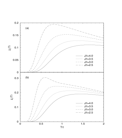
Figure 1: Spin (a) and charge (b) susceptibilities $\chi_{s}$, $\chi_{c}$ vs $T/t$ for the 1D KLM with $U_{c}=0$.

We proceed to calculate the spin susceptibility $\chi_{s}(T)=-\frac{1}{N}{(\frac{\partial^{2}F}{\partial h^{2}})_{h=0}}$, charge susceptibility $\chi_{c}(T)=-\frac{\partial n^{c}}{\partial\mu}$ and specific heat $C(T)=-\frac{1}{N}\beta^{2}\frac{\partial^{2}(\beta F)}{(\partial\beta)^{2}}$. All the thermodynamic quantities are derived from the free energy by a standard procedure. Fig. (1) shows numerical results of spin and charge susceptibilities for the 1D KLM. Raising temperature from zero, both $\chi_{s}(T)$ and $\chi_{c}(T)$ rise exponentially, indicating the existence of the spin and quasiparticle gaps, and then they reach a maximum. The peaks of $\chi_{s}(T)$ and $\chi_{c}(T)$ move to lower temperatures with $J/t$ decreasing, suggesting that the $\Delta_{s}$ and $\Delta_{qp}$ diminish correspondingly. As discussed by Shibata et al.shib and Haule et al.haule , both $\Delta_{s}$ and $\Delta_{qp}$ are responsible for the spin susceptibility but mainly the lower one dominates the low temperature behaviors. In contrast, $\chi_{c}$ is governed by $\Delta_{qp}$ only. Since $\Delta_{qp}<\Delta_{s}$ near the atomic limit, both $\chi_{s}(T)$ and $\chi_{c}(T)$ are dominated by the quasiparticle gap. We find that the activation energies estimated by fitting the spin and charge susceptibilities are similar when $J/t>4$, consistent with the conclusion of the numerical resultsshib ; haule . However the second-order perturbation result is not accurate enough to discuss the delicate relation between the activation energies of $\chi_{s}(T)$ and $\chi_{c}(T)$ and the spin and quasiparticle gaps for smaller couplings.

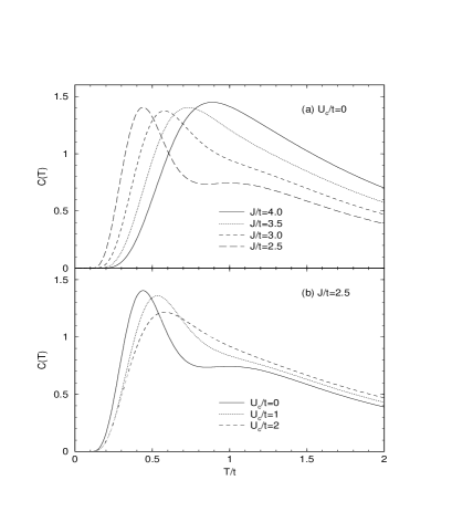
Figure 2: Specific heat $C(T)$ vs $T/t$ of the 1D KLM with (a) $U=0$ and $J/t=4.0,3.5,3.0,2.5$; (b) $J/t=2.5$ and $U_{c}=0,1.0,2.5$.

For $J/t\lesssim 2.5$, there appears an unphysical protrusion on the peak of $\chi_{c}(T)$. This value is an approximate lower limit of the $J/t$ range for which the perturbation theory is reasonable for all temperatures. Within the second-order perturbation theory, the lower limit of $J/t$ is about $2.5$, $3.0$ and $4.0$ for 1D, 2D and 3D KLM’s respectively. This is consistent with the zero-temperature strong-coupling expansions by which the spin gap within second order is given as $\Delta^{(2)}_{s}=J-\frac{20dt^{2}}{3J}$tsun . $\Delta^{(2)}_{s}$ tends to zero quickly at $J/t\approx 2.58,3.65$ and $4.47$ for $d=1,2$ and $3$. Considering higher-order expansions is expected not only to improve the accuracy of the result, also to reduce the lower limit of $J/t$. This task might be achieved by the high order series expansion techniquegelf which has been successful in explaining ground-state properties of KLMshi . The methodology for carrying out high order expansions at finite temperature for spin systems has been developed recentlyelst .

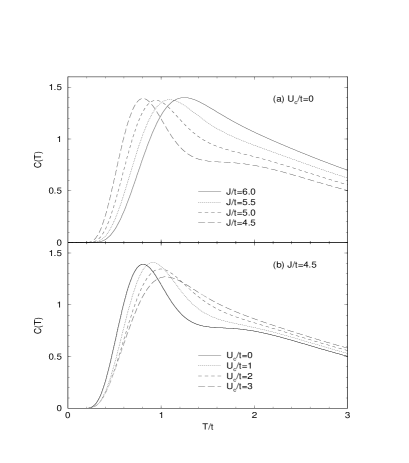
Figure 3: Specific heat of the 3D KLM.

Results of the specific heat for 1D and 3D KLM’s are presented in Figs. (2) and (3). The specific heat contains information on both spin and charge degrees of freedom. The charge fluctuation originates from the movement of conduction electrons. Moving an electron from one site to its neighbors on the ground state background creates a pair of one vacant and one doubly occupied site. The energy cost just is the charge gap. The charge fluctuation is greatly suppressed due to the large charge gap near the atomic limit, so only one peak attributed to the spin excitations can be seen. The location of the peak depends on the spin gap which varies with $J$. The hoping term stirs up the charge fluctuations. Then a new peak originating from the charge degree of freedom begins to be visible as $J/t$ is reduced to $3.0$, as shown in Fig. 2(a). The new peak corresponds to the specific heat of the free conduction electrons and is independent of $J$. The on-site Coulomb repulsion in the conduction electron band will enhance the charge gap and so it suppresses the charge fluctuation. As shown in Fig. 2(b), the second peak in $C(T)$ will vanish with increasing $U_{c}$. Comparing Figs. (3) and (2), the results for the 3D KLM exhibit similar features to those for the 1D case. As the $T=0$ perturbation theory shows, various properties, including the characteristic energy gaps, of the KSL phase are mainly determined by the local dimers in the atomic limittsun , so the dimensionality does not make much difference in thermodynamic properties. This point is also indicated in numerical results for the 2D KLMhaule .

At last, we notice that the above treatment can be also applied to deal with the PAM, but with more complexity. Contrary to the KLM, the charge degrees of freedom of $f$ electrons must be considered in the PAM. The vacancy and double occupancy of the impurity site are possible and thus the Hilbert space of each atom is greatly enlarged. In general case each atom has 16 quantum states. The atomic limit of the PAM has been investigated by many authorsalas ; manc ; noce ; long . Choosing the atom Hamiltonian as the unperturbed Hamiltonian, we can evaluate the thermodynamics near the atomic limit by perturbation theory as above. The physical properties of the PAM are more complicated than those of the KLM. For example, the specific heat will exhibit two peaks even in the atomic limitbern . More recently, Moskalenko et al. calculated the one-particle Green’s function of the PAM by the hopping perturbation treatmentmosk .

In summary, we have studied thermodynamic properties of the Kondo spin liquid phase of the half-filled Kondo lattice model by a finite-temperature perturbation theory. The chemical potential, spin and charge susceptibilities and specific heat are calculated. The results are consistent qualitatively with those obtained by numerical methods. It proves that the strong coupling limit is a reasonable starting point to study thermodynamics of the Kondo spin liquid phase. The accuracy of obtained results is expected to be improved by taking higher-order expansions into account.

The author would like to thank P. Thalmeier for helpful discussions.

Appendix A

The free energy per site within second-order perturbation is given as

$$f(\beta,h)=-\frac{1}{\beta}\left[ln(z_{0})+d\frac{z_{2}}{z_{0}^{2}}\right],$$

where $d=1,2,3$ is the dimensionality and

$$z_{0} = \left[1+e^{-\beta(U_{c}-2\mu n^{c})}\right]f(h)+e^{-\beta(-\frac{3J}{4}-\mu n^{c})}+e^{-\beta(\frac{J}{4}-\mu n^{c})}\left[1+f(2h)\right],$$

$$z_{2} = \frac{\beta^{2}t^{2}}{4}\left[e^{-\beta(-\frac{3J}{4}-\mu n^{c})}+e^{-\beta(-\frac{3J}{4}+U_{c}-3\mu n^{c})}\right]f(h)+\frac{5\beta^{2}t^{2}}{4}\left[e^{-\beta(\frac{J}{4}-\mu n^{c})}+e^{-\beta(\frac{J}{4}+U_{c}-3\mu n^{c})}\right]f(h)$$

$$+ \beta^{2}t^{2}\left[e^{-\beta(\frac{J}{4}-\mu n^{c})}+e^{-\beta(\frac{J}{4}+U_{c}-3\mu n^{c})}\right]f(3h)$$

$$+ \frac{3\beta t^{2}}{2J}\left[e^{-\beta(-\frac{3J}{4}-\mu n^{c})}+e^{-\beta(-\frac{3J}{4}+U_{c}-3\mu n^{c})}-e^{-\beta(\frac{J}{4}-\mu n^{c})}-e^{-\beta(\frac{J}{4}+U_{c}-3\mu n^{c})}\right]f(h)$$

$$- \frac{\beta t^{2}}{J-2U_{c}}\left[4e^{-\beta(\frac{J}{2}-2\mu n^{c})}f(2h)+10e^{-\beta(\frac{J}{2}-2\mu n^{c})}-10e^{-\beta(U_{c}-2\mu n^{c})}\right]$$

$$+ \frac{4\beta t^{2}}{J+2U_{c}}\left[e^{-\beta(-\frac{J}{2}-2\mu n^{c})}f(2h)+e^{-\beta(-\frac{J}{2}-2\mu n^{c})}-e^{-\beta(U_{c}-2\mu n^{c})}\right]$$

$$+ \frac{2\beta t^{2}}{3J+2U_{c}}\left[e^{-\beta(-\frac{3J}{2}-2\mu n^{c})}-e^{-\beta(U_{c}-2\mu n^{c})}\right]+\frac{16\beta t^{2}U_{c}}{J^{2}-4U_{c}^{2}}e^{-\beta(U_{c}-2\mu n^{2})}f(2h)$$

with $f(h)=e^{-\frac{1}{2}\beta h}+e^{\frac{1}{2}\beta h}$.

References

- (1) P.A. Lee, T.M. Rice, J.W. Serene, L.J. Shamand, and J.W. Wilkins, Comments Condens. Matter Phys. 12, 99 (1986).
- (2) P. Fulde, J. Keller, and G. Zwicknagl, Solid State Phys. 41, 1 (1988).
- (3) A.C. Hewson, The Kondo Problem to Heavy Fermions, (Cambridge University Press, Cambridge, 1997).
- (4) J.R. Schriefer and P.A. Wolff, Phys. Rev. 149, 491 (1966).
- (5) H. Tsunetsugu, M. Sigrist, and K. Ueda, Rev. Mod. Phys. 69, 809 (1997).
- (6) Z. Wang, X.P. Li, and D.H. Lee, Physica B 199-200, 463 (1994).
- (7) Z.P. Shi, R.R.P. Singh, M.P. Gelfand, and Z. Wang, Phys. Rev. B 51, 15630 (1995).
- (8) F.F. Assaad, Phys. Rev. Lett. 83, 796 (1999); S. Capponi and F.F. Assaad, Phys. Rev. B 63, 155114 (2001).
- (9) N. Shibata, B. Ammon, M. Troyer, M. Sigrist, and K. Ueda, J. Phys. Soc. Jpn. 67, 1086 (1988); N. Shibata and K. Ueda, J. Phys.: Condens. Matter 11, R1 (1999).
- (10) K. Haule, J. Bonča and P. Prelovšek, Phys. Rev. B 61, 2482 (2000).
- (11) Q. Gu and J.-L. Shen, Phys. Lett. A 150, 251 (1999); Q. Gu, D.-K. Yu, and J.-L. Shen, Phys. Rev. B 60, 3009 (1999).
- (12) D.C. Johnston, M. Troyer, S. Miyahara, D. Lidsky, K. Ueda, M. Azuma, Z. Hiroi, M. Takano, M. Isobe, Y. Ueda, M.A. Korotin, V.I. Anisimov, A.V. Mahajan, and L.L. Miller, cond-mat/0001147
- (13) M. Sigrist, H. Tsunetsugu, K. Ueda, and T.M. Rice, Phys. Rev. B 46, 13838 (1992).
- (14) C. Jurecka and W. Brenig, Phys. Rev. B 64, 092406 (2001).
- (15) R. Eder, O. Stoica, and G.A. Sawatzky, Phys. Rev. B 55, R6109 (1997); R. Eder, O. Rogojanu, and G.A. Sawatzky, ibid. 58, 7599 (1998).
- (16) M.P. Gelfand and R.R.P. Singh, Adv. Phys. 49, 93 (2000).
- (17) N. Elstner and R.R.P. Singh, Phys. Rev. B 57, 7740 (1998).
- (18) B.R. Alascio, R. Allub, and A. Aligia, J. Phys. C 13, 2869 (1980).
- (19) F. Mancini, M. Marinaro, and Y. Nakano, Physica B 159, 330 (1989).
- (20) C. Noce and A. Romano, J. Phys.: Condens. Matter 1, 8347 (1989); Physica B 160, 304 (1990).
- (21) M.W. Long, Z. Phys. B: Condens. Matter 71, 23 (1988).
- (22) U. Bernstein and P. Pincus, Phys. Rev. B 10, 3626 (1974).
- (23) V.A. Moskalenko, P. Entel, M. Marinaro, N.B. Perkins and C. Holtfort, Phys. Rev. B 63, 245119 (2001).