Dynamically Coupled Oscillators – Cooperative Behavior via Dynamical Interaction –

Abstract

We propose a theoretical framework to study the cooperative behavior of dynamically coupled oscillators (DCOs) that possess dynamical interactions. Then, to understand synchronization phenomena in networks of interneurons which possess inhibitory interactions, we propose a DCO model with dynamics of interactions that tend to cause 180-degree phase lags. Employing an approach developed here, we demonstrate that although our model displays synchronization at high frequencies, it does not exhibit synchronization at low frequencies because this dynamical interaction does not cause a phase lag sufficiently large to cancel the effect of the inhibition. We interpret the disappearance of synchronization in our model with decreasing frequency as describing the breakdown of synchronization in the interneuron network of the CA1 area below the critical frequency of 20 Hz.

Many studies of cooperative behavior in many-body systems, of which one prototype is represented by spin systems, have been based on the assumption that the dynamics of interactions can be ignored. However, in the modeling of many biological systems, the inclusion of interaction dynamics is necessary to obtain a faithful description. In much of the research that has been done, systems with such slow interaction have been mimicked by a so-called multi-compartment model which corresponds to a discrete version of a distributed parameter system. By using such a multi-compartment model, we can accurately estimate the dynamical behavior of a single unit. However, it is impossible to carry out a large-scale numerical simulation with such models to understand the behavior of a large-scale system composed of tens of thousands of units. Even if it is possible, we cannot understand the essence of such phenomena. To address this problem, we need to reduce the degrees of freedom needed in a descriptive model.

Phase reduction is a powerful tool that helps us understand the oscillatory behavior of large-scale systems composed of such multi-compartment models. In previous studies of systems consisting of such multi-compartment models, phase descriptions of the entire systems including the dynamical interactions themselves were obtained numerically D.Hansel et al. (1993); Vreeswijk et al. (1994); Crook et al. (1997, 1998). Thus, the effects of the interaction dynamics were numerically incorporated into only a phase-coupling function to establish the phase equation. Therefore, in general, the effects of the interaction dynamics alone cannot be extracted in such methods.

In this paper, we analyze systems of dynamically coupled oscillators (DCOs), and demonstrate how the dynamics of the interactions influence the cooperative behavior exhibited by the systems. Using the multi-scale perturbation method (MSPM) Ermentrout (1981); Kuramoto (1984) to carry out a phase reduction, we are able to represent the nonlinear dynamical interaction in terms of only the amplitude and phase of the fundamental frequency component in the frequency response of the interaction. In control engineering, the amplitude and phase of the fundamental frequency component of the frequency response are referred to as the describing function. The describing function used in the treatment of non-linear systems is an extension of the transfer function used in the treatment of linear systems. In contrast to previous work D.Hansel et al. (1993); Vreeswijk et al. (1994); Crook et al. (1997, 1998), the effects of the interaction dynamics are expressed by the describing function in our approach, and so it is easy to isolate and extract the effects of the interaction dynamics from the phase equation. Therefore, our approach can clearly elucidate the effect of the interaction dynamics on the cooperative behavior of entire systems. Our results imply the possibility of a new modeling approach for biological systems by which the describing function of the interaction is identified. The description proposed here corresponds more to higher order approximation than to conventional linear description (e.g., the auto-regressive (AR) model).

In the first half of this paper, we show in detail the process of analytical phase reduction for a general model with dynamical interaction. We treat a large population of Stuart-Landau (SL) oscillators coupled through nonlinear dynamical interaction. The SL oscillators have the essential structure of the Hopf-bifurcation, because its evolution equation can be derived from any non-linear oscillator system with the Hopf-bifurcation through perturbation expansion Kuramoto (1984). In the latter half of the paper, we apply our theoretical framework to the analysis of a network of interneurons. The analysis of an interneuron network is a good example to verify the applicability of our approach for understanding the neural cooperative behavior via dynamical interaction.

First, we consider a large population of SL oscillators weakly coupled through interactions which themselves are nonlinear dynamical systems. We analyze the following coupled system:

$$\frac{dw_{j}}{dt}=w_{j}\left(1-|w_{j}|^{2}\right)+i\left(\Omega+\epsilon\omega_{j}\right)w_{j}+\frac{\epsilon}{N}\sum_{k=1}^{N}s_{jk}.$$ (1)

Here $w_{j}$ is the state variable (a complex number) of the $j$th oscillator (with a total of $N$). $\Omega$ is the average natural frequency and $\epsilon\omega_{j}$ represents the deviation from the average for the $j$th oscillator randomly distributed with a density represented by $g(\omega)$. The terms multiplied by $\epsilon$ are considered perturbations, and thus, the quantity $\epsilon$ controls the magnitude of perturbations. When $\epsilon=0$, the system has an unstable fixed point at the origin and a stable limit-cycle orbit on the unit circle in the complex plane represented by

$$w_{j}(t)=\Phi_{j}(t),\ \Phi_{j}(t)=\exp i\left(\Omega t+\phi_{j}\right),\ ^{\forall}\phi_{j}\in{\bf R}/2\pi,$$ (2)

where $\phi_{j}$ is the phase of the $j$th oscillator. When $\epsilon=0$, the system is neutrally stable with respect to a perturbation in the form of a temporal shift while it conserves a fixed orbit. Thus, $\phi_{j}$ depends only on the initial condition. The quantity $s_{jk}$ in Eq. (1) represents the output from the dynamical system of the interaction expressed by

$$s_{jk}=V_{jk}(x_{jk},w_{k}),\ \ \frac{dx_{jk}}{dt} = F_{jk}\left(x_{jk},w_{k}\right),$$ (3)

where $x_{jk}$ represents the internal state of the interaction, $F_{jk}(\cdot)$ is a nonlinear function determining its dynamics, and $V_{jk}(\cdot)$ is an output function.

We now discuss the dynamical interaction described by Eq. (3). If $w_{k}=\Phi_{k}(t)=\exp i\left(\Omega t+\phi_{k}\right)$ is input into Eq. (3), the higher harmonics resulting from the nonlinearity of this equation are superimposed on $s_{jk}$. Here we restrict our consideration to the case that the output $s_{jk}$ is a periodic function possessing the same period as the input $w_{k}$. In this case, $s_{jk}$ can be expanded into the following Fourier form: $s_{jk}=J_{jk}^{(1)}\Phi_{k}+\sum_{n>1}^{\infty}J_{jk}^{(n)}\Phi_{k}^{n}$. If Eq. (3) takes a form of a linear system, $J_{jk}^{(1)}$ would be non-zero, and $J_{jk}^{(n)}$ for $n>1$ would all be zero. In this case, $J_{jk}^{(1)}$ is called the transfer function of the dynamical interaction Eq. (3). If, on the other hand, Eq. (3) takes a form of a nonlinear system, $J_{jk}^{(1)}$ and some of $J_{jk}^{(n)}$ for $n>1$ would be non-zero. In this case, $J_{jk}^{(1)}$ is called the describing function in the field of control engineering.

Now, employing the MSPM, we attempt to reduce Eq. (1) to a phase equation. The solution of the perturbed system (1) can be represented as

$$w_{j}(t)=\Phi_{j}(t)+\epsilon u_{j}(t),\ \Phi_{j}(t)=\exp i\left(\Omega t+\phi_{j}(\epsilon t)\right),$$ (4)

where we write $\phi_{j}$ as a function of $\epsilon t$ to make explicit its slow evolution in time, and $\epsilon u_{j}$ is the first order change in $w_{j}$ introduced by the perturbation. If we substitute Eq. (4) into Eqs. (1) and (3) and expand the resulting expression about $\epsilon=0$, the $O(\epsilon)$ equation becomes

$$i\Phi_{j}\frac{d\phi_{j}}{d(\epsilon t)} = i\omega_{j}\Phi_{j}+{\it L}_{\phi_{j}}u_{j}+\frac{1}{N}\sum_{n=1}^{\infty}\sum_{k=1}^{N}J_{jk}^{(n)}\Phi_{k}^{n}.$$ (5)

Here ${\it L}_{\phi}$ is the linear operator corresponding to Eq. (1) linearized about the periodic solution (2) in the case $\epsilon=0$. It is given by

$${\it L}_{\phi}u=-\frac{du}{dt}+i\Omega u-\Phi^{2}\overline{u}-u,$$ (6)

where the overline denotes complex conjugation. All of the eigenvalues of ${\it L}_{\phi}$ are non-positive, since the solution $\Phi(t)$ is stable. Note that there exists the eigenfunction $\Phi^{\prime}(t)$ of ${\it L}_{\phi}$ with eigenvalue $0$. This eigenfunction corresponds to an infinitesimal temporal shift because $\Phi(t+\delta)\sim\Phi(t)+\delta\Phi^{\prime}(t)$. We assume there exists no other eigenfunction with eigenvalue $0$ in the space of the periodic functions, so that ${\rm ker}{\it L}_{\phi}={\rm span}\{\Phi^{\prime}(t)\}={\rm span}\{i\Phi(t)\}$. This assumption is equivalent to that of the orbital stability of $\Phi(t)$.

We define the inner product of two $\frac{2\pi}{\Omega}$-periodic complex functions $u(t)$ and $v(t)$ as $\left<u(t),v(t)\right>=\int_{0}^{\frac{2\pi}{\Omega}}dt\left({\rm Re}\{u(t)\}{\rm Re}\{v(t)\}+{\rm Im}\{u(t)\}{\rm Im}\{v(t)\}\right)$. Then, we obtain the operator adjoint to $L_{\phi}$ as

$${\it L}_{\phi}^{\ast}u=\frac{du}{dt}-i\Omega u-\Phi^{2}\overline{u}-u.$$ (7)

From Fredholm’s alternative Ermentrout (1981), there is a so-called response function $\Phi^{\ast}(t)$ that spans the kernel of $L^{\ast}_{\phi}$ in the space of periodic functions. Therefore, ${\rm ker}{\it L}_{\phi}^{\ast}={\rm span}\{\Phi^{\ast}(t)\}$. In this case, we explicitly obtain $\Phi^{\ast}(t)=i\Phi(t)$. Taking the inner product of $i\Phi(t)$ and Eq. (5), we obtain

$$\left<i\Phi_{j},i\Phi_{j}\right>\frac{d\phi_{j}}{d(\epsilon t)}-\left<i\Phi_{j},i\Phi_{j}\right>\omega_{j}-\frac{1}{N}\sum_{k,n}\left<i\Phi_{j},J_{jk}^{(n)}\Phi_{k}^{n}\right>$$

$$=\left<i\Phi_{j},{\it L}_{\phi_{j}}u_{j}\right>=\left<{\it L}_{\phi_{j}}^{\ast}i\Phi_{j},u_{j}\right>=0,$$ (8)

where the quantity $\epsilon t$ is treated as a constant over a single period, since $\phi_{j}(\epsilon t)$ is driven by a weak perturbation. Here, the higher harmonics resulting from the nonlinearity of Eq. (3) cancel, because $\left<i\Phi_{j},J_{jk}^{(n)}\Phi_{k}^{n}\right>=0\ (n>1)$. Thus, we derive the phase equation describing the slow phase dynamics of the system,

$$\frac{d\phi_{j}}{d(\epsilon t)}=\omega_{j}+\frac{1}{N}\sum_{j}^{N}A_{jk}\sin\left(\phi_{k}-\phi_{j}+\psi_{jk}\right),$$ (9)

$${\rm with}\ A_{jk}=|J_{jk}^{(1)}|,\ \ \psi_{jk}=\arg J_{jk}^{(1)},$$ (10)

where $\omega_{j}$ represents a natural frequency of unit $j$ at the level of the phase equation. As Eqs. (9) and (10) reveal, in the phase equation, the dynamical interaction (3) is expressed in terms of the describing function. Thus, seen the fundamental frequency components in the output from the dynamical system of the interaction (3) clearly play a key role in the slow phase dynamics of the system.

If all interactions are identical, i.e. $J_{jk}^{(1)}=J$ ($A_{jk}=A$ and $\psi_{jk}=\psi$), Eq. (9) is equivalent to the Sakaguchi-Kuramoto model Sakaguchi and Kuramoto (1986), and so, in this case, the Sakaguchi-Kuramoto theory can be applied to the analysis of Eq. (9). Here, we define the mean field as $m=\frac{1}{N}\sum_{j=1}^{N}w_{j}$. When $|m|\neq 0$, the system is in a state of phase synchronization. In the thermodynamic limit, $N\rightarrow\infty$, we obtain the following self-consistent equation relating the order parameters $|m|$ and $\tilde{\Omega}$:

$$|m|e^{i\psi} = A|m|\int_{-\pi/2}^{\pi/2}d\phi g\left(\tilde{\Omega}+|m|\sin\phi\right)\cos\phi\exp(i\phi)$$ (11)

$$+ iA|m|\int_{0}^{\pi/2}d\phi\frac{\cos\phi(1-\cos\phi)}{\sin^{3}\phi}$$

$$\times\left\{g\left(\tilde{\Omega}+\frac{|m|}{\sin\phi}\right)-g\left(\tilde{\Omega}-\frac{|m|}{\sin\phi}\right)\right\}.$$

Here, to derive the order parameter equation, we have assumed the existence of one large cluster of oscillators phase-locked at frequency $\tilde{\Omega}$ in the slow dynamics described by (9). In the original system, described by (1), the frequency of the synchronous cluster is $\Omega+\epsilon\tilde{\Omega}$.

(a)
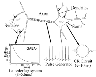
(b) (c)

Figure 1: (a) Dynamical behavior of neural components. (b) Schematic diagram of the dynamical interaction employed in our model which consists of a rectangular-pulse generator and a second-order lag system (SOLS). (c) Bode diagram of the SOLS, $G(i\Omega)=1/(1+i\Omega\tau)^{2}$.

Next, we apply our theoretical framework to the analysis of a network of interneurons as an example. High frequency oscillations, known as $\gamma$ oscillations, have been observed in many areas of the brain. The synchronization of inhibitory interneurons is known to be the origin of $\gamma$ oscillations Whittington et al. (1995). Inhibitory interactions, which correspond to anti-ferromagnetic interactions in spin systems, introduce competition; for this reason, in general, such interactions tend to prevent synchronization. Therefore, the synchronization phenomena in networks of interneurons are non-trivial Vreeswijk et al. (1994); Ernst et al. (1995); Wang and Buzsáki (1996). A series of physiological in vitro experiments inspired our study. One in particular was the experimental discovery that the interneuronal network in the CA1 area of the hippocampus displays synchronization at frequencies greater than or close to 20 Hz, but not at frequencies significantly below this value Traub et al. (1996a, b). The discovery of this phenomenon provides evidence suggesting that cooperative behavior in networks of interneurons arises due to the dynamical nature of the interactions.

To understand the mechanism of the synchronization, we propose a DCO model with interaction dynamics that tend to cause 180-degree phase lags. The estimated connectivity between interneurons in the CA1 area is 10% Wang and Buzsáki (1996). The interneuron network in the CA1 area has dense connectivity, because the number of connections between interneurons is $O(N)$. Therefore, we can capture properties of the interneuron network by analyzing the global coupling systems. As shown in Fig. 1(b), the dynamical interactions of neurons are modeled by a rectangular-pulse generator consisting of a threshold element and a second-order lag system (SOLS):

$$s_{jk}=-x_{jk}^{(1)},\ \left[\begin{array}[]{c}\tau^{(1)}_{jk}\frac{dx_{jk}^{(1)}}{dt}\\ \tau^{(2)}_{jk}\frac{dx_{jk}^{(2)}}{dt}\end{array}\right]=\left[\begin{array}[]{cc}-1&1\\ 0&-1\end{array}\right]\left[\begin{array}[]{c}x_{jk}^{(1)}\\ x_{jk}^{(2)}\end{array}\right]$$ (18)

$$+\left[\begin{array}[]{c}0\\ G\end{array}\right]\Theta\left({\rm Re}\{w_{k}\}-H\right),\ \Theta(x)=\left\{\begin{array}[]{cc}1&x>0\\ 0&x\leq 0\end{array}\right..$$ (23)

The parameters $\tau^{(1)}_{jk}$ and $\tau^{(2)}_{jk}$ are the time constants of the two cascade units of the first-order lag system that form the SOLS. In Eq. (23), the parameters $G$ and $H$ denote, respectively, the gain and the threshold of the threshold element, and are defined as $G=1/\theta$ and $H=\cos\theta$ $(\theta>0)$. If the value of $\theta$ is small, the rectangular pulse generated by the threshold element is sharp. Note that Eq. (23) represents mutual interactions only between the real parts of the SL oscillators.

In the context of control engineering, the SOLS is regarded as one of the minimal models for realizing a 180-degree phase lag. As shown in Fig. 1(a), the electrical properties of somata and proximal dendrites can be approximated as the CR circuit. Near resting potential, we can obtain a linear approximation of their behavior as being that of a first-order lag system. The response of the synaptic conductance is also displayed in Fig. 1(a). The evolution of the synaptic conductance is roughly reproduced by that of the first-order lag system. Thus, as shown in Fig. 1(a), the SOLS given by Eq. (23) can be considered as a cascade system consisting of these components. In addition, to model the generation of action potentials in a neuron when its membrane potential reaches the threshold, and furthermore, to demonstrate the applicability of our approach in analyses of non-linear systems, we have also introduced a threshold element into the dynamical interaction given in Eq. (23).

The describing function for the dynamical interaction given in (23) is

$$J_{jk}^{(1)} = -\frac{2\sin\theta}{\pi\theta}\cdot\frac{1}{(1+i\tau^{(1)}_{jk}\Omega)(1+i\tau^{(2)}_{jk}\Omega)}.$$ (24)

Here, the describing function of the threshold element is $2\sin\theta/(\pi\theta)$, which contributes only to the gain of Eq. (24). Figure 1(c) displays the Bode diagrams of the SOLS. As Fig. 1(c) reveals, the gain of the SOLS, which is a type of low-pass filter, is a decreasing function of frequency at high frequencies, while the phase of the SOLS converges to -180 degrees as the frequency increases. If the phase lag is 180 degrees, $J_{jk}^{(1)}$ is a positive real number, and the system thus effectively becomes a ferromagnetic oscillator system. Note that Eq. (23) represents the mutual interactions only between the real parts of the SL oscillators. Thus, $A_{jk}$ takes half the value it had in Eq. (10), and here $A_{jk}=\frac{1}{2}|J_{jk}^{(1)}|,\ \ \psi_{jk}=\arg J_{jk}^{(1)}$.

(a) (b)

Figure 2: (a) $|m|$ as a function of $\sigma$. The data points with error bars represent the means and standard deviations of 10 samples obtained from numerical simulations of Eq. (1). Here, $\Omega=2\pi 80$, $\tau=0.02$, $\theta=\pi/6$, $\epsilon=10$ and $N=1000$. (b) Critical deviation $\sigma_{c}$ as a function of $\Omega\tau$. The quantity plotted here is actually a normalized critical deviation, with maximum value $1$.

In the numerical calculation we will now discuss, we chose the distribution of natural frequencies as $g(\omega)=(2\pi\sigma^{2})^{-1/2}\exp\left(-\omega^{2}/(2\sigma^{2})\right)$, where $\sigma$ is the deviation of the natural frequencies. We begin with systems where the interactions are all equivalent, i.e., $\Omega\tau^{(1)}_{jk}=\Omega,\tau^{(2)}_{jk}=\Omega\tau$, and hence $A_{jk}=A$ and $\psi_{jk}=\psi$. In this case, Eq. (9) is equivalent to the Sakaguchi-Kuramoto model Sakaguchi and Kuramoto (1986). Figure 2(a) displays $|m|$ as a function of $\sigma$ in the case of the dynamical interaction given by Eq. (23), where the solid curves were obtained from the order parameter equation (11), and the data points with error bars represent results obtained using the fourth-order Runge-Kutta method with Eqs. (1) and (23). Next, we estimate the critical value of $\sigma$, representing the boundary between $|m|=0$ and $|m|\neq 0$. Figure 2(b) displays the critical deviation $\sigma_{c}$ as a function of $\Omega\tau$ for the two models. Note that the absolute values of $A$ and $\sigma_{c}$ have no meaning in comparing such models, because $\sigma_{c}$ is proportional to $A$ Sakaguchi and Kuramoto (1986). Plotted in Fig. 2(b) is the critical deviation normalized to have a maximum value of $1$. The widths of the synchronous regions decrease as the frequency increases because, as shown in Fig. 1(c), the SOLS is a low-pass filter whose gain rapidly decreases at higher frequencies. However, if $G$ in Eq. (23) is sufficiently large, the gain of the interaction given by Eq. (23) can be made sufficiently large by the pulse generator to realize synchronization at high frequencies. However, as Fig. 2(b) reveals, our model does not exhibit synchronization at low frequencies because, as shown in Fig. 1(c), this dynamical interaction does not cause a phase lag sufficiently large to cancel the effect of the inhibition. We interpret the disappearance of synchronization in our model with decreasing frequency as describing the breakdown of synchronization in the interneuron network of the CA1 area below the critical frequency of 20 Hz Traub et al. (1996a, b). Based on this correspondence, we conjecture that in an interneuron network, a phase lag resulting from the dynamical nature of the interactions might cancel the effect of inhibition at high frequencies, and through this cancellation, the system effectively becomes a ferromagnetic oscillator system.

Figure 3: System size scaling. Deviation of local fields multiplied by $\sqrt{N}$ as a function of $N$.

By means of numerical simulations, as shown in Fig. 3, we have demonstrated through a scaling plot that the variation of a local field is $O(1/\sqrt{N})$ in systems where a quenched random time constant is used for the interaction dynamics in Eq. (23). In the thermodynamical limit $N\rightarrow\infty$, the system asymptotically approaches a system with global homogeneous interaction, even with a quenched random time constant of the interaction dynamics. Therefore, as the system size $N$ increases, the system tends to synchronize through the cancellation of fluctuation via interaction.

References

- D.Hansel et al. (1993) D.Hansel, G. Mato, and C. Meunier, Europhysics Letters 23, 367 (1993).
- Vreeswijk et al. (1994) C. V. Vreeswijk, L. F. Abbott, and G. B. Ermentrout, J. Computational Neuroscience 1, 313 (1994).
- Crook et al. (1997) S. M. Crook, G. B. Ermentrout, M. C. Vanier, and J. M. Bower, J. Computational Neuroscience 4, 161 (1997).
- Crook et al. (1998) S. M. Crook, G. B. Ermentrout, and J. M. Bower, J. Computational Neuroscience 5, 315 (1998).
- Ermentrout (1981) G. B. Ermentrout, Journal of Mathematical Biology 6, 327 (1981).
- Kuramoto (1984) Y. Kuramoto, Chemical oscillations, waves and turbulence (Springer-Verlag, 1984).
- Sakaguchi and Kuramoto (1986) H. Sakaguchi and Y. Kuramoto, Pro. of Theo. Phys. 76, 576 (1986).
- Whittington et al. (1995) M. A. Whittington, R. D. Traub, and J. G. R. Jefferys, Nature 373, 612 (1995).
- Ernst et al. (1995) U. Ernst, K. Pawelzik, and T. Geisel, Phys. Rev. Let. 74, 1570 (1995).
- Wang and Buzsáki (1996) X. Wang and G. Buzsáki, J. Neuroscience 16, 6402 (1996).
- Traub et al. (1996a) R. D. Traub, M. A. Whittington, I. M. Stanford, and J. G. R. Jefferys, Nature 383, 621 (1996a).
- Traub et al. (1996b) R. D. Traub, M. A. Whittington, S. B. Colling, G. Buzsaki, and J. G. R. Jefferys, J. Physiology 493, 471 (1996b).