Vortex viscosity in the moderately clean limit of layered superconductors

Abstract

We present a microscopic calculation of the energy dissipation in the core of a vortex moving in a two-dimensional or layered superconductor in the moderately clean regime. In this regime, the quasiclassical Bardeen–Stephen result remains valid in spite of the strong correlations between the energy levels. We find that the quasiclassical expression applies both in the limit of fast vortex motion (with transitions between smeared levels) and in the limit of slow vortex motion (with nearly adiabatic dynamics). This finding can be related to the similar result known for the unitary random-matrix model.

I Introduction

At low temperature the energy dissipation in the vortex cores is the main source of resistivity in the mixed state of type-II superconductorsLarkin-Ovchinnikov . If a supercurrent flows through a superconductor, it exerts a force on the vortices. Unless pinned by impurities or inhomogeneities, the vortices are brought into motion, which in turn leads to dissipation. Depending on the level of disorder, the vortices may move at different angles with respect to the direction of the supercurrent. At weak disorder, the vortices move together with the supercurrent (“ballistic limit”, with the Hall angle close to $\pi/2$). At sufficiently strong disorder, the vortex motion is directed perpendicular to the supercurrent (“dissipative limit”, small Hall angle). Both limits are well understood within the quasiclassical description GK73 ; Bardeen-Sherman ; LO76 ; Kopnin-Kravtsov ; Kopnin94 ; Kopnin-Lopatin . A simplified approach describing the dissipative limit goes back to the theory of Bardeen and Stephen treating the vortex as a region of normal phase inside a superconductor Bardeen-Stephen . In spite of neglecting the structure of the quasiparticle excitations in the vortex core CDGM , the Bardeen–Stephen theory gives the same result (up to a numerical factor) as the accurate quasiclassical calculation GK73 ; Bardeen-Sherman ; LO76 ; Kopnin-Kravtsov ; Kopnin94 ; Kopnin-Lopatin .

It has been recently suggested that the microscopic structure of the core excitations may play a much more prominent role in that part of the dissipative regime where the excitation spectrum remains discrete (sharp quasiparticle levels), specifically in layered superconductorsFS ; LO98 ; KL ; GP . In the clean limit (i.e., for scattering rates $\hbar/\tau$ much smaller than the superconducting gap $\Delta$), the motion of quasiparticles in the vortex core is ballistic: they cross the vortex core many times before scattering off impurities. Therefore in this limit the spectral properties are sensitive to the details of disorder realization. In the superclean regime ($\hbar/\tau\ll\Delta^{2}/E_{F}$, where $E_{F}$ is the Fermi energy) the levels inside a two-dimensional vortex split into two sets (‘combs’) of equally spaced levels LO98 . The transformation of this correlated spectrum into a featureless uncorrelated one with increasing disorder proceeds in distinct steps: within the moderately clean regime ($\Delta^{2}/E_{F}\ll\hbar/\tau\ll\Delta$) a new intermediate region ($\Delta^{2}/E_{F}\ll\hbar/\tau\ll\Delta\sqrt{\Delta/E_{F}}$) has been found LO98 ; KL where the comb structure remains preserved but is randomly shifted in energy (the number of impurities in the core has to be small enough to preserve the ‘combs’, while being large enough to randomize the overall shift). Increasing the impurity concentration further (already in the moderately clean limit for weak impurities SKF , and ultimately in the dirty limit Zirnbauer ), the ‘comb’ structure is destroyed with a crossover to the class $C$ random-matrix ensembleAZ .

Keeping within the moderately clean regime with a discrete spectrum, in two-dimensional (or layered) superconductors there further exist two limits of dissipation FS : The first one applies to the slowly moving vortex with a discrete quasiparticle spectrum (“discrete-spectrum regime”) where the dissipation is due to Landau–Zener transitions between individual levels LZ ; Wilkinson . The second limit is with levels smeared into a continuum either by the vortex motion or by inelastic processes (“continuum-spectrum regime”); the dissipation then is given by the linear-response Kubo formula Kubo . At low temperatures, the inelastic smearing can be neglected and the crossover between these two regimes is controlled by the vortex velocity with the characteristic velocity given by $v_{K}\sim(\Delta/p_{F})/\sqrt{k_{F}l}$ (here, $\Delta$ is the superconducting gap and $l$ denotes the elastic mean free pathFS ).

In the framework of random-matrix models with time-dependent Hamiltonians, the dissipation in the discrete-spectrum and continuum-spectrum regimes was considered by Wilkinson Wilkinson . He finds that, in the case of the unitary Wigner–Dyson ensemble, the linear dissipative response remains valid in the whole range of velocities, both in the continuum-spectrum (high velocity) and in the discrete-spectrum (low velocity) regimes. Based on this fact and on the similarity between the unitary and class $C$ ensembles, it was shown that with the class $C$ level statistics the dissipation rate nearly follows the Bardeen-Stephen prediction, even in the limit of small velocities $v<v_{K}$ where the quasiclassical description is no longer valid FS . Contrary, it was claimed in Ref. KL, that the additional correlation between levels (the ‘two-comb’ structure) may lead to an anomalously high vortex viscosity in the moderately clean regime in the low-velocity limit.

In our paper, we reconsider the problem of the vortex viscosity in a two-dimensional $s$-wave superconductor, taking full account of the discreteness of the vortex spectrum and of the microscopic structure of the quasiparticle levels. We assume the moderately clean limit with an appropriate number of impurities in the core, such that the spectrum possesses the randomly shifted two-comb structure (the precise condition is given in Section III). We find that in spite of the level correlations derived in Refs. LO98, ; KL, , the vortex viscosity does not differ from the well-known quasiclassical result GK73 ; Bardeen-Sherman ; LO76 ; Kopnin-Kravtsov ; Kopnin94 ; Kopnin-Lopatin for three-dimensional superconductors. Within the same microscopic model we consider separately the discrete-spectrum and continuum-spectrum regimes of dissipation: in both limits we arrive at the Bardeen–Stephen result for the dissipation,

$$\sigma_{xx}=\frac{ecn\omega_{0}\tau}{B}\sim\sigma_{n}\frac{H_{c2}}{B},$$ (1)

where $n$ is the electron density, $\hbar\omega_{0}\sim\Delta^{2}/E_{F}$ is the spacing between the levels in the coreCDGM , and $B$ is the magnetic field. The two-comb level structure found in Refs. LO98, ; KL, may be classified as the circular unitary random-matrix ensemble of dimension twoMehta . Therefore our findings may be considered as a generalization of Wilkinson’s results Wilkinson to circular ensembles. We also find the scattering time $\tau$ for quasiparticles in the core in the $s$-wave approximation: for a weak impurity strength, the effective $1/\tau$ is larger than the bulk scattering rate $1/\tau_{n}$ by the logarithm of the impurity strength. A similar logarithmic correction was previously derived in Refs. Kopnin94, ; Kopnin-Lopatin, .

The paper is organized as follows. In Section II we prepare for the calculation by deriving the microscopic Hamiltonian projected onto the relevant subgap states in the vortex core. In Section III we review the results of Refs. LO98, ; KL, on the circular random-matrix ensemble appearing in a disordered vortex at the intermediate level disorder. We then describe the two limiting regimes of dissipation (Sect. IV), the discrete-spectrum and the continuum-spectrum regimes, and set up the stage for the calculations. In Section V we treat the case of the discrete energy spectrum (low velocities and no inelastic level broadening), while Section VI is devoted to the opposite continuum-spectrum limit where the levels are broader than the interlevel distance. Finally, we discuss our findings in Section VII. The sensitivity of the energy levels to the vortex displacement is calculated in an Appendix.

II Microscopic Hamiltonian of the moving vortex

Before discussing the moving vortex, let us review the excitation spectrum of a clean two-dimensional vortex at rest. The corresponding wave functions are given by the solutions to the Bogoliubov–deGennes equations

$$\begin{pmatrix}H_{0}&\Delta({\bf r})\\ \Delta^{*}({\bf r})&-H_{0}\end{pmatrix}\begin{pmatrix}u\\ v\end{pmatrix}=E\begin{pmatrix}u\\ v\end{pmatrix},$$ (2)

where $H_{0}={\bf p}^{2}/2m-E_{F}$. We assume an axially symmetric vortex with the order parameter $\Delta({\bf r})=\Delta(r)e^{i\theta}$, where the modulus of the order parameter depends only on the radial component $r$ and the phase winds with the angular coordinate $\theta$. We neglect the magnetic field in the vortex core, assuming a large magnetic penetration depth $\lambda\gg\xi$, where $\xi=v_{F}/\pi\Delta$ is the superconducting coherence length (here and below we choose units with $\hbar=1$). In the quasiclassical limit $k_{F}\xi\gg 1$, the spectrum and the eigenfunctions may be easily foundCDGM . The eigenvalues form a spectrum of equidistant levels

$$E_{\mu}=\mu\omega_{0},$$ (3)

where the angular momentum $\mu$ takes half-integer values, $\mu=n+1/2$, and

$$\omega_{0}=\frac{\int_{0}^{\infty}\frac{\Delta(r)}{k_{F}r}e^{-2K(r)}\,dr}{\int_{0}^{\infty}e^{-2K(r)}\,dr},$$ (4)

$$K(r)=\int_{0}^{r}\frac{\Delta(r^{\prime})}{v_{F}}\,dr^{\prime};$$ (5)

$r$ is the distance from the core center. The basic electronic energy scale in the vortex core takes the value $\omega_{0}\sim\Delta^{2}/\varepsilon_{F}$, up to a possible logarithmic prefactor $\log(\Delta/T)$ due to the shrinkage of the vortex core at small temperatures $T$ (Kramer–Pesch effectKramer-Pesch ). The eigenstates $\Psi_{\mu}=(u_{\mu},v_{\mu})^{T}$ take the form

$$\Psi_{\mu}({\bf r})={\cal A}\begin{pmatrix}J_{\mu-1/2}(k_{F}r)\,e^{-i(\mu-1/2)\theta}\\ J_{\mu+1/2}(k_{F}r)\,e^{-i(\mu+1/2)\theta}\end{pmatrix}e^{-K(r)},$$ (6)

where ${\cal A}^{2}=[4k_{F}^{-1}\int_{0}^{\infty}e^{-2K(r)}dr]^{-1}\sim k_{F}/\xi$ is the normalization factor, and $J_{n}(x)$ are the Bessel functions.

In the following, we will be interested in processes at energies far below the superconducting gap and thus project all the operators onto the subgap states (6). It will be convenient to take the Fourier transform of these eigenvectors in the variable $\mu$ and introduce a new angular variable $\phi$ labelling the direction of the quasiclassical motion of the quasiparticle,

$$\Psi_{\phi}({\bf r})\equiv\sum_{\mu}\Psi_{\mu}({\bf r})\,e^{i\mu\phi}={\cal A}\begin{pmatrix}e^{i\phi/2}\\ e^{-i\phi/2}\end{pmatrix}e^{-K(r)}e^{i{\bf k}_{\phi}{\bf r}},$$ (7)

where we introduced the vector ${\bf k}_{\phi}=k_{F}(\sin\phi,-\cos\phi)$ pointing perpendicular to the direction specified by the angle $\phi$, with absolute value $k_{F}$. The plane-wave exponent in (7) is then ${\bf k}_{\phi}{\bf r}=k_{F}r\sin(\phi-\theta)$. This basis of wave functions has a very simple structure: in addition to the phase winding $\exp(\pm i\phi/2)$ (providing the antiperiodic boundary conditions in $\phi$), these wave functions are plane waves in the direction of the wave vector ${\bf k}_{\phi}$ restricted to a region of size $\xi$ around the vortex center. Note that $\Psi_{\phi}({\bf r})$ is not an eigenfunction of the Hamiltonian (2). Prepared in such a state at $t=0$, the wave function will rotate in the $\phi$-basis according to $\Psi({\bf r},t)=\Psi_{\phi-\omega_{0}t}({\bf r})$.

We now turn to the problem of the moving vortex with impurities. It can be described by the time-dependent Bogoliubov–deGennes equations

$$i\frac{\partial}{\partial t}\Psi=H(t)\Psi,$$ (8)

where $H(t)$ is the Hamiltonian of the vortex at the position ${\bf r}={\bf v}t$ with ${\bf v}$ the vortex velocity,

$$H(t)=\begin{pmatrix}H_{0}+U({\bf r})&\Delta({\bf r}-{\bf v}t)\\ \Delta^{*}({\bf r}-{\bf v}t)&-H_{0}-U({\bf r})\end{pmatrix},$$ (9)

and $U({\bf r})$ is the potential set up by the impurities.

In the clean limit ($\Delta\tau\gg 1$), the admixture of bulk states (with energies greater than $\Delta$) to the vortex states may be neglected. We project the Hamiltonian (9) onto the subgap states of a clean vortex (7) by substituting

$$\Psi({\bf r},t)=\int_{0}^{2\pi}\frac{d\phi}{2\pi}a(\phi,t)\Psi_{\phi}({\bf r}-{\bf v}t).$$ (10)

Defined in this way, the amplitude $a(\phi,t)$ has antiperiodic boundary conditions in $\phi$, $a(\phi+2\pi)=-a(\phi)$. The time evolution of the coefficients $a(\phi,t)$ obeys the Schrödinger-type equation

$$i\frac{\partial}{\partial t}a=-i\omega_{0}\frac{\partial}{\partial\phi}a+\int\frac{d\phi^{\prime}}{2\pi}T_{\phi\phi^{\prime}}a(\phi^{\prime})+\int\frac{d\phi^{\prime}}{2\pi}L_{\phi\phi^{\prime}}a(\phi^{\prime}),$$ (11)

where the kernel

$$T_{\phi\phi^{\prime}} =\left\langle\Psi_{\phi}({\bf r}-{\bf v}t)\right|\left(-i\frac{\partial}{\partial t}\right)\left|\Psi_{\phi^{\prime}}({\bf r}-{\bf v}t)\right\rangle$$

$$=i{\bf v}\left\langle\Psi_{\phi}\right|\nabla\left|\Psi_{\phi^{\prime}}\right\rangle$$ (12)

is produced by the vortex motion, and the kernel

$$L_{\phi\phi^{\prime}}=\left\langle\Psi_{\phi}({\bf r}-{\bf v}t)\right|U({\bf r})\tau_{z}\left|\Psi_{\phi^{\prime}}({\bf r}-{\bf v}t)\right\rangle$$ (13)

is due to the impurities.

The $T$-kernel may be easily computed from the explicit form (7) of $\Psi_{\phi}$. In the limit $k_{F}\xi\gg 1$, the matrix element (12) takes the form

$$T_{\phi\phi^{\prime}}=-2\pi\delta(\phi-\phi^{\prime})\,{\bf k}_{\phi}{\bf v}$$ (14)

and we identify this term with the “Doppler shift”.

The impurity potential $U({\bf r})$ is taken as a sum over point-like impurities,

$$U({\bf r})=\sum_{i}V_{i}\,\delta({\bf r}-{\bf r}_{i}).$$ (15)

Then the scattering kernel may be expressed as KL ; SKF

$$L_{\phi\phi^{\prime}}\!=\!2i{\cal A}^{2}\!\sin\frac{\phi^{\prime}{-}\phi}{2}\,\sum_{i}V_{i}e^{-2K(|{\bf r}_{i}-{\bf v}t|)}e^{i({\bf k}_{\phi^{\prime}}-{\bf k}_{\phi})({\bf r}_{i}-{\bf v}t)}.$$ (16)

Summarizing, we end up with the equation of motion (11) containing three terms: The first term describes the circular (“chiral”) motion of the quasiparticle in the vortexCDGM ; LO98 ; KL . The second term is the Doppler shift due to the vortex motion. And the third term describes the scattering off impurities (taking point-like impurities is equivalent to including only $s$-wave scattering). We are interested in the energy pumping in this time-dependent model. Note that the physical energy is given by the first and third terms in the evolution operator (11) but does not include the second term ($T$-term) which arises from the time-derivative of the basis wave functions. This discrepancy between the energy and the evolution operator may be resolved by an appropriate time-dependent gauge transformation

$$\tilde{a}(\phi)=a(\phi)e^{-i{\bf k}_{\phi}{\bf v}t}.$$ (17)

This gauge transformation has a dual effect on the equation of motion (11): Firstly, it makes the energy operator coincide with the evolution operator. The old $T$-kernel is now replaced by a time-dependent one,

$$\tilde{T}_{\phi\phi^{\prime}}=2\pi\delta(\phi-\phi^{\prime})\>\omega_{0}({\bf n}_{z}\times{\bf k}_{\phi}){\bf v}t,$$ (18)

where ${\bf n}_{z}$ is the unit vector perpendicular to the plane (this gauge transformation resembles the one in electrodynamics replacing a static electric field with a magnetic field linearly growing in time). Secondly, the $L$-kernel is transformed as well and the new kernel takes the form

$$\tilde{L}_{\phi\phi^{\prime}}=2i{\cal A}^{2}\sin\frac{\phi^{\prime}-\phi}{2}\,\sum_{i}V_{i}e^{-2K(|{\bf r}_{i}-{\bf v}t|)}e^{i({\bf k}_{\phi^{\prime}}-{\bf k}_{\phi}){\bf r}_{i}},$$ (19)

which differs from Eq. (16) by the cancellation of the velocity term ${\bf v}t$ in the last exponent.

The physical content of the two gauges may be understood in the following way: The basis wave functions (7) are quasiclassical plane waves (at the wave vector $k_{F}$) cut off by the long-wavelength envelope $\exp(-2K(r))$ of the size of order $\xi$. In the original gauge [with variables $a(\phi,t)$], this basis was chosen by simply translating the basis (7) together with the vortex. In the new gauge [with variables $\tilde{a}(\phi,t)$], only the long-wavelength envelope is translated, without shifting the phases of the quasiclassical plane waves.

This difference in matching phases of plane waves at different vortex positions produces two different descriptions of the moving vortex. In the first gauge [variables $a(\phi,t)$], the evolution equation (11) contains impurities moving with respect to the vortex (fast oscillations in $L_{\phi\phi^{\prime}}$). This description is similar to the approach taken in Refs. FS, ; LO98, ; KL, , a static vortex subject to moving impurities. However, in those references, the $T$-term was omitted. We will show below that omitting this term does not change the result for the dissipation in the moderately clean limit, thus justifying the approach of Refs. FS, ; LO98, ; KL, . In the second gauge [variables $\tilde{a}(\phi,t)$], there are no oscillating terms in $L_{\phi\phi^{\prime}}$ (except for the slowly varying envelope $K(r)$ whose time derivative may be neglected in most cases). All the oscillations in the $L$-term in the first gauge may be removed by a single gauge transformation, as all impurities move with respect to the vortex with the same velocity and in the same direction. This fact has not been properly taken into account in Ref. KL, , which has lead to an unphysical result. We shall comment in more detail on the derivation of Ref. KL, in Sec. V; here we just remark that the parallel motion of the impurities with respect to the vortex requires special care in the calculations within the first gauge, but is automatically taken into account in the second gauge.

III Circular unitary ensemble of the quasiparticle levels in the disordered vortex

In this section, we review the derivation of the two-comb spectral statistics in the vortex from Refs. LO98, ; KL, and set up the notation for the calculations in the later sections. For the discussion of the spectral statistics in this section we take the vortex at rest (${\bf v}=0$). Then the Hamiltonian in the equation of motion (11) contains only two terms, the kinetic term $-i\omega_{0}\partial/\partial\phi$ and the scattering term $L_{\phi\phi^{\prime}}$ (for a vortex at rest there is no difference between $L_{\phi\phi^{\prime}}$ and $\tilde{L}_{\phi\phi^{\prime}}$).

At not very high impurity concentration [see Eq. (38) below], the scattering kernel $L_{\phi\phi^{\prime}}$ may be approximated as a sum of two local terms [this approximation is due to the rapidly oscillating exponent in (16)],

$$L_{\phi\phi^{\prime}}=4\pi i\omega_{0}\sum_{i=1}^{N}[J_{i}\check{\delta}_{\phi,\phi_{i}}\check{\delta}_{\phi^{\prime},\phi_{i}+\pi}-J_{i}^{*}\check{\delta}_{\phi,\phi_{i}+\pi}\check{\delta}_{\phi^{\prime},\phi_{i}}],$$ (20)

where $N$ is the number of impurities in the core, the parameters $\phi_{i}$ specify the angular positions of the impurities, and $\check{\delta}_{\phi_{1},\phi_{2}}$ are $\delta$-functions smeared over the width $(\phi_{1}-\phi_{2})\sim(k_{F}\xi)^{-1/2}$ and antiperiodically continued in $\phi_{1}$ and $\phi_{2}$ ($\check{\delta}_{\phi_{1},\phi_{2}+2\pi}=\check{\delta}_{\phi_{1}+2\pi,\phi_{2}}=-\check{\delta}_{\phi_{1},\phi_{2}}$). Note that the regularization (20) as a product of two smeared $\delta$-functions is important for evaluating the scattering matrix (24) below LO98 ; KL . The effective strength of the $i$-th impurity is

$$J_{i}=\frac{i{\cal A}^{2}V_{i}e^{-2K(r_{i})+2ik_{F}r_{i}}}{\omega_{0}k_{F}r_{i}}\sim i\vartheta_{i}\frac{\xi}{r_{i}}e^{-2K(r_{i})+2ik_{F}r_{i}},$$ (21)

where $\vartheta_{i}=mV_{i}$ is the Born parameter of the impurity (an additional imaginary unit compared to the notation in Ref. KL, is due to the antiperiodic boundary conditions employed).

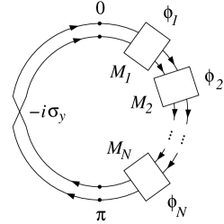
Figure 1: Schematic representation of the evolution of the wave function $\psi(\phi)$ in the circular-unitary-ensemble regime. The two-component wave function $\psi(\phi)$ rotates with the angular velocity $\omega_{0}$ and scatters off impurities. The impurity scattering is local and is described by the unitary matrices $M_{i}$, according to (23). After rotating by half a turn, the wave function is projected back to the origin with the help of the boundary condition (25).

The matrix elements (20) couple only angles with difference close to $\pi$. Introducing the two-component vector

$$\psi(\phi)=\begin{pmatrix}a(\phi)\\ a(\phi+\pi)\end{pmatrix},\qquad\phi\in[0;\pi],$$ (22)

the scattering becomes local in $\phi$. The individual scattering events in (11) then may be integrated separately and formulated in terms of a boundary condition KL

$$\psi(\phi_{i}+0)=M_{i}\psi(\phi_{i}-0),$$ (23)

where

$$M_{i}=\frac{1}{1+|J_{i}|^{2}}\begin{pmatrix}1-|J_{i}|^{2}&2J_{i}\\ -2J_{i}^{*}&1-|J_{i}|^{2}\end{pmatrix}.$$ (24)

The boundary condition for $\psi(\phi)$ going around the half circle is

$$\psi(0)=-i\sigma_{y}\psi(\pi).$$ (25)

Thus the energy levels are determined by the eigenvalues of the matrix $-i\sigma_{y}M$, where

$$M=M_{N}\dots M_{2}M_{1},\quad\pi>\phi_{N}>\dots>\phi_{1}>0.$$ (26)

The full “scattering matrix” $-i\sigma_{y}M$ is a unitary matrix with the eigenvalues $\exp(\pm i\pi E/\omega_{0})$, so that the energy levels $E$ are solutions to the equation

$$\cos(\pi E/\omega_{0})=-\frac{i}{2}\mathop{\rm tr}\sigma_{y}M.$$ (27)

The evolution of the wave function $\psi(\phi)$ is schematically shown in Fig. 1.

In the moderately clean limit with a sufficiently large (but not too large) number of impurities in the core, the matrix $M$ (and thus also $-i\sigma_{y}M$) is random with a uniform distribution over the $SU(2)$ group. Such a random-matrix ensemble is classified as the “circular unitary” ensemble with dimension two Mehta . The density of states and the level correlations may be easily computed from Eq. (27). For example, the average density of states is given byKL

$$\langle\rho(E)\rangle=\frac{2}{\omega_{0}}\sin^{2}\left(\pi\frac{E}{\omega_{0}}\right).$$ (28)

The spectrum consists of two combs of equidistant levels: A level is characterized by the comb number $s=\pm 1$ and its position in the comb, $E_{\pm,k}=\pm(E_{0}+2\omega_{0}k)$, where $E_{0}$ is the eigenvalue of the lowest level with positive energy ($0\leq E_{0}<\omega_{0}$). The eigenfunctions can be written explicitly as

$$\psi_{\pm,k}(\phi)=e^{i\phi E_{\pm,k}/\omega_{0}}M_{\phi,0}\psi_{\pm}(\phi=0),$$ (29)

where $\psi_{\pm}(\phi=0)$ are the two eigenvectors of $-i\sigma_{y}M$, and the scattering matrices $M_{\phi,\phi^{\prime}}$ are defined as

$$M_{\phi,\phi^{\prime}}=M_{i_{n}}\dots M_{i_{1}},\quad\phi>\phi_{i_{n}}>\dots>\phi_{i_{1}}>\phi^{\prime},$$ (30)

where the product is taken over all impurities between the angles $\phi^{\prime}$ and $\phi$. Eq. (30) introduces $M_{\phi,\phi^{\prime}}$ for $\phi>\phi^{\prime}$; furthermore, it is convenient to define the scattering matrix for $\phi<\phi^{\prime}$ as $M_{\phi,\phi^{\prime}}=M_{\phi^{\prime},\phi}^{\dagger}$. The symmetry of the $SU(2)$ matrices

$$M_{\phi,\phi^{\prime}}^{*}=\sigma_{y}M_{\phi,\phi^{\prime}}\sigma_{y}$$ (31)

allows us to translate easily between the eigenfunctions for the two series of levels via

$$\psi_{-,-k}(\phi)=\sigma_{y}\psi_{+,k}^{*}(\phi).$$ (32)

In our calculations, we shall need not only the properties of the spectrum, but also some statistical properties of the wave functions in the regime of the circular unitary ensemble. At any given point $\phi$ and for any energy level, the wave function $\psi(\phi)$ is a spinor pointing in a random direction. All directions are equally probable, allowing us to compute equal-point correlation functions such as

$$\langle\psi^{\dagger}(\phi)\sigma_{\alpha}\psi(\phi)\cdot\psi^{\dagger}(\phi)\sigma_{\beta}\psi(\phi)\rangle =\frac{\delta_{\alpha\beta}}{3},$$ (33a)

$$\langle\psi^{\dagger}(\phi)\sigma_{\alpha}\psi^{*}(\phi)\cdot\psi^{T}(\phi)\sigma_{\beta}\psi(\phi)\rangle =\frac{2\delta_{\alpha\beta}}{3}.$$ (33b)

The correlations between wave functions at different values of $\phi$ may be expressed in terms of the properties of the scattering matrices (30). The angular correlations between scattering matrices decay exponentially,

$$\langle M^{\dagger}_{\phi,\phi^{\prime}}\sigma_{z}M_{\phi,\phi^{\prime}}\rangle=e^{-|\phi-\phi^{\prime}|/\phi_{\tau}}\sigma_{z},$$ (34)

where

$$\frac{1}{\omega_{0}\tau}\equiv\frac{1}{\phi_{\tau}}=16n_{\rm imp}\int_{0}^{\infty}r\,dr\frac{|J(r)|^{2}}{(1+|J(r)|^{2})^{2}},$$ (35)

and $n_{\rm imp}$ is the impurity concentration. In (35) we have assumed (for simplicity) that all impurities have equal Born parameters, in which case the effective impurity strength $J_{i}$ as given by (21) becomes a function of $r_{i}$ and is denoted $J(r)$ in (35). In order to derive (34) and (35) one takes a small increment of $\langle M^{\dagger}_{\phi,\phi^{\prime}}\sigma_{z}M_{\phi,\phi^{\prime}}\rangle$ in $\phi$ and averages over a single impurity scattering matrix,

$$\frac{\partial}{\partial\phi}\langle M^{\dagger}_{\phi,\phi^{\prime}}\sigma_{z}M_{\phi,\phi^{\prime}}\rangle=2n_{\rm imp}\int_{0}^{\infty}r_{i}\,dr_{i}\\ {}\times\left[\langle M^{\dagger}_{\phi,\phi^{\prime}}M_{i}^{\dagger}\sigma_{z}M_{i}M_{\phi,\phi^{\prime}}\rangle-\langle M^{\dagger}_{\phi,\phi^{\prime}}\sigma_{z}M_{\phi,\phi^{\prime}}\rangle\right].$$ (36)

The last averaging is performed independently over $M_{\phi,\phi^{\prime}}$ and $M_{i}$. In averaging, we first account for the rapidly oscillating off-diagonal elements in (24) and arrive at (34), (35).

For strong impurities with the Born parameter $\vartheta\equiv mV_{i}\sim 1$ (as above, we assume that all impurities are of equal strength), the scattering time $\tau$ is of the order of the bulk normal-state elastic mean-free time $\tau_{n}$. For weak impurities with $\vartheta\ll 1$, the integral in Eq. (35) has a logarithmic dependence on the Born parameterKL ,

$$\frac{1}{\tau}\sim\frac{1}{\tau_{n}}\ln\frac{1}{\vartheta}.$$ (37)

A similar logarithmic behavior of the scattering rate was also derived in Refs. Kopnin94, ; Kopnin-Lopatin, . The relaxation angle $\phi_{\tau}$ in (35) plays a central role in the context of vortex dissipation, as it enters the expression for the friction coefficient and hence also for the flux flow conductivity. In Ref. KL, this quantity entered the numerator in the expression for the conductivity, while in our results it enters the denominator in the Bardeen–Stephen form (1). We comment in detail on our disagreement with Ref. KL, in Section V and in the Appendix.

The physical meaning of $\phi_{\tau}$ is the correlation length of the scattering matrix $M_{\phi,\phi^{\prime}}$ and $\tau$ is the corresponding scattering time. We shall see later that it is the correlation function (34) which determines the rate of interlevel transitions. In principle, one can derive a similar exponential decay “in the $x$ and $y$ directions” [with $\sigma_{z}$ replaced by $\sigma_{x}$ or $\sigma_{y}$ in (34)], in which case the correlation length $\phi_{\tau}^{(xy)}$ is twice larger than $\phi_{\tau}$ “in the $z$ direction”. This is due to the specific form (24) of the scattering matrix $M_{i}$.

In order to realize the regime of the circular unitary random-matrix ensemble it is necessary that $\phi_{\tau}\ll\pi$, which defines the lower bound for the moderately clean regime, $\omega_{0}\tau\ll 1$. However, the region of the circular unitary ensemble does not extend over the whole moderately clean regime KL . The additional restriction originates from the breaking of the instant-scattering approximation (20) in the limit of too strong disorder. Indeed, the typical width of the smeared $\check{\delta}$-functions in this equation can be estimated as $\delta\phi\sim 1/\sqrt{k_{F}\xi}$ (that corresponds to an impurity at the distance of the order of $\xi$ from the vortex center). On the other hand, the number of impurities in the core is $N\sim n_{\rm imp}\xi^{2}\sim 1/\omega_{0}\tau_{n}\vartheta^{2}$. The solution for the spectrum discussed above is justified as long as the $\check{\delta}$-functions in Eq. (20) do not overlap, which is equivalent to the condition $N\,\delta\phi\ll 1$. Thus, the circular unitary ensemble is realized only in a relatively narrow range of disorder strengths

$$\frac{\omega_{0}}{\ln 1/\vartheta}\ll\frac{1}{\tau_{n}}\ll\vartheta^{2}\sqrt{\Delta\omega_{0}}$$ (38)

[we assume that the Born parameter $\vartheta\ll 1$ and make use of Eq. (37); for $\vartheta\sim 1$ one should replace $\ln 1/\vartheta$ by 1]. For stronger disorder (i.e., larger scattering rate $1/\tau_{n}$) or smaller Born parameter $\vartheta$ the instant-scattering approximation (20) fails and the circular unitary ensemble crosses over to the class $C$ ensemble Zirnbauer ; SKF . A phenomenological approach to this crossover has been discussed in Ref. BHL, and the results of numerical simulations are available in Ref. Fujita, .

IV Two regimes of dissipation

The time evolution of the core states is described by Eq. (11). Since the evolution operator is nonstationary (i.e., explicitly time-dependent), it causes transitions between levels with different energy. In a fermionic system, the rate of downward transitions is suppressed compared to the rate of upward transitions due to the Pauli exclusion principle, leading to an increase of the average energy with time. The energy pumped into the system will finally be transferred to the thermal bath via the interaction with phonons or other soft degrees of freedom, thus producing a finite dissipation.

There are two different mechanisms of dissipation depending on whether the individual energy levels can be resolved or not Wilkinson . If the discrete spectrum is smeared into a continuous one, the energy pumping can be calculated with the help of the standard linear-response Kubo formula Kubo . This regime is naturally realized when the inelastic width $\gamma_{\rm in}$ of an energy level exceeds the mean level spacing $\omega_{0}$. On the other hand, the spectrum may turn out effectively continuous even at $\gamma_{\rm in}\ll\omega_{0}$ if the time dependence of the evolution operator on the right-hand side of Eq. (11) is so fast that it destroys the instantaneous adiabatic spectrum Wilkinson . In this case, the frequency $\gamma_{v}$ of perturbations due to the nonadiabaticity of the spectrum exceeds $\omega_{0}$ and plays the role of the effective level width. In the opposite case, when $\gamma_{\rm in},\gamma_{v}\ll\omega_{0}$, the spectrum is essentially discrete and the dissipation is due to rare Landau–Zener transitions LZ taking place when two levels come very close to each other.

In a normal metal at low temperatures, the inelastic widths due to the electron-electron and electron-phonon interactions are given by $\gamma_{e-e}\sim T^{2}/E_{F}$ and $\gamma_{e-ph}\sim T^{3}/\Theta_{D}^{2}$, respectivelyinelastic ($\Theta_{D}$ is the Debye temperature). Since $\gamma_{e-e}$ is of the order of $\omega_{0}$ already at $T\sim\Delta$, it does not contribute to the level smearing at lower temperatures. Furthermore, for the states localized in the vortex core the interaction with phonons appears to be strongly suppressed compared to the normal-state rate e-ph ; one of the main reasons is that the quasiparticles with energy $\mu\omega_{0}\ll\Delta$ are composed of nearly equal mixtures of electron and hole components [i.e., $\langle u_{\mu}^{2}\rangle\approx\langle v_{\mu}^{2}\rangle$, cf. Eq. (6)] with negligible net charge. Thus, at sufficiently small temperatures $T\ll\Delta$, the inelastic width of the core states $\gamma_{\rm in}\ll\omega_{0}$ and the regime of dissipation is determined solely by the vortex velocity. In Ref. FS, the crossover velocity $v_{K}$ separating the regimes with discrete and continuous spectra was estimated as

$$v_{K}\sim\frac{\Delta/p_{F}}{\sqrt{k_{F}l}}$$ (39)

and we will present a microscopic derivation of this result below.

For model Hamiltonians from the three Wigner-Dyson random-matrix ensembles Mehta , dissipation was calculated by Wilkinson Wilkinson ; Wilkinson-comment in the regimes of small ($v\ll v_{K}$) and large ($v\gg v_{K}$) velocities (in the limit $\gamma_{\rm in}=0$). He finds that if the Hamiltonian $H(X)$ of the system depends on time through $X=vt$ then the energy dissipation is determined by the variance of the (off-diagonal, $i\neq k$) matrix elements $C(0)\equiv\left\langle|\partial H_{ik}/\partial X|^{2}\right\rangle/\omega_{0}^{2}$ normalized by the mean level spacing $\omega_{0}$. In the continuous-spectrum regime specified by $v\gg v_{K}\equiv\omega_{0}C^{-1/2}(0)$, the energy dissipation rate as given by the Kubo formula,

$$W_{\rm Kubo}=\pi C(0)v^{2},$$ (40)

is the same for the orthogonal ($\beta=1$), unitary ($\beta=2$), and symplectic ($\beta=4$) ensembles and describes viscous damping. In the discrete-spectrum regime, at $v\ll v_{K}$, the result depends on the level-repulsion parameter $\beta$, which determines the probability $P(\varepsilon)\propto\varepsilon^{\beta}$ to find two levels at a distance $\varepsilon\ll\omega_{0}$. In this situation the energy dissipation rate is given by the expression Wilkinson

$$W_{\beta}\propto v^{(\beta+2)/2},$$ (41)

hence the dissipation is superohmic for the Gaussian orthogonal ensemble, while for the Gaussian unitary ensemble it remains ohmic with $W_{2}=\pi C(0)v^{2}$, exactly coinciding with $W_{\rm Kubo}$ despite a very different mechanism of dissipation.

In the next sections we calculate the dissipation rate for the vortex motion in the regime of the Koulakov–Larkin ‘two-comb’ spectrum KL , both in the limits of small and large velocities, thus extending Wilkinson’s considerations to the case of circular unitary ensembles.

V Dissipation in the discrete spectrum (Landau–Zener regime)

In this section we calculate the dissipation for the two-comb level structure described in Section III at small velocities. We will work in the ‘tilded’ basis $\tilde{a}(\phi,t)$ introduced in Eq. (17), where the energy coincides with the expectation value of the evolution operator (11), with $T_{\phi\phi^{\prime}}$ and $L_{\phi\phi^{\prime}}$ substituted by their tilded counterparts (18) and (19). In the low-velocity limit, the energy is pumped into the system when two levels come very close to each other and a nonadiabatic Landau–Zener transition becomes possible. Due to the symmetry of the two-comb spectrum the rate $R_{\rm\scriptscriptstyle LZ}$ of such transitions is the same for each neighboring pair of levels. We will calculate $R_{\rm\scriptscriptstyle LZ}$ by considering the lowest level with positive energy $\varepsilon$ and its mirror image with energy $-\varepsilon$. For simplicity we assume that the vortex moves in the $x$ direction, $v_{y}=0$.

Following the logic of Ref. Wilkinson, , we diagonalize the Hamiltonian at $t=0$ and restrict it to the $2\times 2$ matrix involving the pair of states considered,

$$\tilde{H}(t)=\begin{pmatrix}\varepsilon+h_{11}t&h_{12}t\\ h_{12}^{*}t&-\varepsilon-h_{11}t\end{pmatrix},$$ (42)

where $h_{ij}$ are the elements of the matrix $\partial H/\partial t$ (neglecting the quadratic term $\propto(\partial^{2}H/\partial t^{2})t^{2}$ is justified in the Landau–Zener regime since the duration of a nonadiabatic transition is proportional to the gap of the avoided crossing and is small at $v\ll v_{K}$). The instantaneous adiabatic spectrum takes the form

$$E(t)=\pm\sqrt{\Delta_{\rm\scriptscriptstyle LZ}^{2}+A^{2}(t-t_{\rm\scriptscriptstyle LZ})^{2}},$$ (43)

where

$$\Delta_{\rm\scriptscriptstyle LZ}^{2}=\frac{\varepsilon^{2}|h_{12}|^{2}}{A^{2}},\quad A^{2}=h_{11}^{2}+|h_{12}|^{2},\quad t_{\rm\scriptscriptstyle LZ}=-\frac{\varepsilon h_{11}}{A^{2}}.$$ (44)

Equation (43) describes an avoided crossing with the minimal distance (Landau–Zener gap) $2\Delta_{\rm\scriptscriptstyle LZ}$ between the spectral branches realized at $t=t_{\rm\scriptscriptstyle LZ}$. The probability of the Landau–Zener transition at such a crossing is $\exp(-\pi\Delta_{\rm\scriptscriptstyle LZ}^{2}/A)$. The mean rate of transitions is given by

$$R_{\rm\scriptscriptstyle LZ}=\left\langle\delta(t_{\rm\scriptscriptstyle LZ})\exp\left(-\pi\frac{\Delta_{\rm\scriptscriptstyle LZ}^{2}}{A}\right)\right\rangle,$$ (45)

where the role of $\delta(t_{\rm\scriptscriptstyle LZ})$ is to count each avoided crossing once. The average in Eq. (45) is taken over the distribution of the parameters $\varepsilon$, $h_{11}$, and $h_{12}$ describing the avoided crossing. The energy $\varepsilon$ is expressed through the transfer matrix $M$ according to Eq. (27). The coefficients $h_{11}$ and $h_{12}$ are the matrix elements of the perturbation (18) over the exact wave functions $\psi_{\pm}(\phi)\equiv\psi_{\pm,0}(\phi)$ [which depend on the trajectory $M_{\phi,0}$ via Eq. (29)],

$$h_{11}=\omega_{0}k_{F}v\int_{0}^{\pi}\frac{d\phi}{\pi}\psi_{+}^{\dagger}(\phi)\sigma_{z}\psi_{+}(\phi)\cos\phi,$$ (46)

$$h_{12}=\omega_{0}k_{F}v\int_{0}^{\pi}\frac{d\phi}{\pi}\psi_{+}^{\dagger}(\phi)\sigma_{z}\psi_{-}(\phi)\cos\phi.$$ (47)

We come to the crucial point: The quantities $\varepsilon$, $h_{11}$, and $h_{12}$ have different dependencies on the transfer matrix $M_{\phi,0}$. In the moderately clean limit, when the number of impurities in the core is sufficiently large and $\phi_{\tau}\ll 1$, the matrix $M_{\phi,0}$ performs many rotations over the $SU(2)$ group. Therefore, we conclude that (i) $\varepsilon$, $h_{11}$, and $h_{12}$ are uncorrelated, and (ii) the distribution of $h_{11}$ and $h_{12}$ is Gaussian. We further calculate the variances of $h_{11}$ and $h_{12}$. For $\langle h_{11}^{2}\rangle$ we obtain with the help of Eq. (34),

$$\langle h_{11}^{2}\rangle={} (\omega_{0}k_{F}v)^{2}\int_{0}^{\pi}\frac{d\phi}{\pi}\frac{d\phi^{\prime}}{\pi}\cos\phi\cos\phi^{\prime}e^{-|\phi-\phi^{\prime}|/\phi_{\tau}}$$

$${}\times\langle\psi_{+}^{\dagger}(\phi)\sigma_{z}\psi_{+}(\phi)\cdot\psi_{+}^{\dagger}(\phi)\sigma_{z}\psi_{+}(\phi)\rangle.$$ (48)

Integrating over $\phi-\phi^{\prime}$ and averaging over the spinor $\psi(\phi)$ according to (33a) we find

$$\frac{\langle h_{11}^{2}\rangle}{(\omega_{0}k_{F}v)^{2}}=\frac{\phi_{\tau}}{\pi}\left\langle(\psi_{+}^{\dagger}\sigma_{z}\psi_{+})^{2}\right\rangle=\frac{\phi_{\tau}}{3\pi}.$$ (49)

Analogously, with the help of Eq. (33b) we obtain

$$\frac{\langle|h_{12}|^{2}\rangle}{(\omega_{0}k_{F}v)^{2}}=\frac{\phi_{\tau}}{\pi}\left\langle|\psi_{+}^{\dagger}\sigma_{x}\psi_{+}^{*}|^{2}\right\rangle=\frac{2\phi_{\tau}}{3\pi}.$$ (50)

In the same way it can be shown that $\langle h_{11}h_{12}\rangle=0$, thus proving the statistical independence of $h_{11}$ and $h_{12}$. We conclude that $h_{11}$, $\Re h_{12}$, and $\Im h_{12}$ are independently distributed with the same distribution

$${\cal P}(h)=\sqrt{\frac{3}{2\phi_{\tau}}}\frac{1}{\omega_{0}k_{F}v}\exp\left(-\frac{3\pi h^{2}}{2\phi_{\tau}(\omega_{0}k_{F}v)^{2}}\right).$$ (51)

The distribution function for $\varepsilon$ is provided by the density of states (28), in the limit $\varepsilon\ll\omega_{0}$, ${\cal P}(\varepsilon)=2\pi^{2}\varepsilon^{2}/\omega_{0}^{3}$.

Averaging Eq. (45) over $\varepsilon$, $h_{11}$, and $h_{12}$ with the distributions ${\cal P}(\varepsilon)$ and ${\cal P}(h)$, we obtain for the mean rate of Landau–Zener transitions

$$R_{\rm\scriptscriptstyle LZ}=\frac{k_{F}^{2}v^{2}\phi_{\tau}}{2\omega_{0}}.$$ (52)

The energy dissipation rate is given by $W=\omega_{0}R_{\rm\scriptscriptstyle LZ}\equiv\eta v^{2}$ with the vortex viscosity

$$\eta=\frac{1}{2}k_{F}^{2}\phi_{\tau}=\frac{1}{2}k_{F}^{2}\omega_{0}\tau.$$ (53)

As defined by Eq. (53), $\eta$ is a two-dimensional viscosity. In a layered superconductor, it determines the friction force ${\bf F}=-\eta{\bf v}$ exerted on the vortex from excitation of quasiparticles within one layer.

The statistics (51) of the matrix elements of $\partial H/\partial t$ determines the sensitivity of the spectrum to the vortex motion and allows one to find the critical velocity $v_{K}$ separating the regimes of discrete and continuum spectra. The discrete spectrum can be resolved if the change of the Hamiltonian during the time $\omega_{0}^{-1}$, $\delta H\sim h/\omega_{0}$, is smaller than $\omega_{0}$. Taking for $h$ the dispersion of the distribution (51), we find for the critical vortex velocity

$$v_{K}\sim\frac{\omega_{0}}{k_{F}\sqrt{\phi_{\tau}}},$$ (54)

coinciding with the estimate (39) found in Ref. FS, .

Comparing with Ref. KL, , we find that our result (53) for the viscosity is smaller by a factor $\phi_{\tau}^{2}$ and the expression (54) for $v_{K}$ is larger by the factor $1/\phi_{\tau}$. In Ref. KL, , following the analysis in Refs. FS, ; LO98, , it was assumed that the dissipation is produced by impurities moving with respect to the vortex, equivalent to neglecting the Doppler-shift term $T_{\phi\phi^{\prime}}$ in Eq. (11). In order to identify the origin of the discrepancy in the results and verify the validity of omitting the Doppler shift, we reconsider below the treatment of Ref. KL, — we will see that the source of the disagreement is not in the neglect of the Doppler-shift term but in the neglect of cross-correlations between the motion of different impurities. To demonstrate this, we adopt the approach of Ref. KL, (omitting the Doppler-shift term) and re-calculate the correlator of the spatial gradients of the matrix $M$ KL-comment1

$${\cal C}=\frac{1}{4}\biggl{<}\left(\mathop{\rm tr}\frac{\partial M}{\partial x}\right)^{2}\biggr{>},$$ (55)

from which the viscosity follows via $\eta=2\,{\cal C}/\pi$. Comparison between Eqs. (55) and (40) shows that the quantity $(2/\pi^{2}){\cal C}$ plays the role of the correlation function $C(0)$.

The matrix $M$ specified in Eq. (26) is a product of transfer matrices of individual impurities. Therefore, there are two contributions to the correlator (55), one originating from derivatives over the coordinates of the same impurity (diagonal part) and a second one from derivatives taken on different impurities (off-diagonal part),

$${\cal C}_{\rm diag}=\frac{1}{4}\sum_{i}\left<\mathop{\rm tr}\frac{\partial M}{\partial x_{i}}\mathop{\rm tr}\frac{\partial M}{\partial x_{i}}\right>,$$ (56)

$${\cal C}_{\rm off-diag}=\frac{1}{4}\sum_{i\neq j}\left<\mathop{\rm tr}\frac{\partial M}{\partial x_{i}}\mathop{\rm tr}\frac{\partial M}{\partial x_{j}}\right>.$$ (57)

The diagonal part is given by KL

$${\cal C}_{\rm diag}=\frac{\pi k_{F}^{2}}{4\phi_{\tau}}.$$ (58)

The cross term, expressing the correlated nature of the motion of the impurities with respect to the vortex, has been missed in Ref. KL, . Its calculation is presented in the Appendix and the result takes the form

$${\cal C}_{\rm off-diag}=-\frac{\pi k_{F}^{2}}{4\phi_{\tau}(1+\phi_{\tau}^{2})}.$$ (59)

We thus see that the two contributions ${\cal C}_{\rm diag}$ and ${\cal C}_{\rm off-diag}$ nearly cancel each other and the net sensitivity of the spectrum to the vortex motion appears to be significantly lower than that found in Ref. KL, ,

$${\cal C}=\frac{\pi k_{F}^{2}\phi_{\tau}}{4},$$ (60)

where we employed the condition $\phi_{\tau}\ll 1$ of the moderately clean limit. Using Eq. (55) one recovers the result (53) for the vortex viscosity. The above consideration not only corrects the result of Ref. KL, ; in addition, it serves as a microscopic justification of the model adopted in Refs. FS, ; LO98, ; KL, , where the dissipation is due to impurities moving through the core and the Doppler-shift term $T$ in Eq. (11) is neglected.

VI Dissipation in the continuum spectrum (Kubo formula)

If the vortex velocity $v$ exceeds $v_{K}$ the discrete spectrum is smeared and transitions between non-nearest levels become possible. In this limit, the energy dissipation can be calculated with the help of the Kubo formula; as in Sec. V we will use the ‘tilded’ basis (17). Neglecting the slow time dependence of $\tilde{L}_{\phi\phi^{\prime}}$, we write the evolution operator as $\tilde{H}(t)=H_{0}+It$, where $H_{0}$ is the Hamiltonian of the vortex at rest and $I=\tilde{T}/t$ takes the form

$$I_{\phi\phi^{\prime}}=2\pi\delta(\phi-\phi^{\prime})I(\phi),\qquad I(\phi)=\omega_{0}k_{F}v\cos\phi,$$ (61)

where we again assumed that $v_{y}=0$. The energy dissipation rate

$$W\equiv\frac{dE}{dt}=\langle t|\frac{\partial}{\partial t}\tilde{H}(t)|t\rangle$$ (62)

is calculated as the linear response to the term $It$ with the help of the Kubo formula

$$W=i\int_{-\infty}^{0}t^{\prime}dt^{\prime}\langle 0|[{\cal I}(t^{\prime}),{\cal I}(0)]|0\rangle,$$ (63)

where

$${\cal I}(t)=\int_{0}^{2\pi}I(\phi)\hat{\Psi}^{\dagger}(\phi,t)\hat{\Psi}(\phi,t)\frac{d\phi}{2\pi}$$ (64)

and $\hat{\Psi}(\phi,t)$ is a second-quantized operator in the interaction representation. The latter can be rewritten in terms of the (exact disorder dependent) eigenfunctions $\tilde{a}_{n}(\phi)$ and eigenvalues $E_{n}$ of the Hamiltonian $H_{0}$,

$$\hat{\Psi}(\phi,t)=\sum_{n}\hat{c}_{n}\tilde{a}_{n}(\phi)e^{-iE_{n}t},$$ (65)

with $\hat{c}_{n}$ the corresponding annihilation operators. Averaging over the initial state of the vortex at rest (so that $\tilde{a}_{n}(\phi)$ coincides with $a_{n}(\phi)$) one arrives at the expression

$$W=i\int_{-\infty}^{0}t^{\prime}dt^{\prime}\int\frac{d\phi d\phi^{\prime}}{(2\pi)^{2}}I(\phi)I(\phi^{\prime})\sum_{km}(n_{k}-n_{m})$$

$${}\times a_{k}(\phi)a_{k}^{*}(\phi^{\prime})a_{m}(\phi^{\prime})a_{m}^{*}(\phi)e^{i(E_{k}-E_{m})(t^{\prime}-t)},$$ (66)

where $n_{k}=\langle\hat{c}_{k}^{\dagger}\hat{c}_{k}\rangle$ is the distribution function at the energy $E_{k}$. This expression can readily be represented (cf., e.g., Ref. Mahan, ) in terms of the Green functions

$$G^{R,A}_{E}(\phi,\phi^{\prime})=\sum_{n}\frac{a_{n}(\phi)a_{n}^{*}(\phi^{\prime})}{E-E_{n}\pm i\delta},$$ (67)

$$W=\frac{1}{2}\int\frac{d\phi d\phi^{\prime}}{(2\pi)^{2}}\int\frac{dE}{2\pi}\frac{\partial n(E)}{\partial E}I(\phi)I(\phi^{\prime})$$

$${}\times[G^{R}_{E}(\phi\phi^{\prime})-G^{A}_{E}(\phi\phi^{\prime})][G^{R}_{E}(\phi^{\prime}\phi)-G^{A}_{E}(\phi^{\prime}\phi)].$$ (68)

The above formula for the dissipation rate is not restricted to the regime of the circular unitary ensemble but is valid in the whole moderately clean limit regime as long as $v\gg v_{K}$. In particular, one can easily recover the result of the standard quasiclassical analysis by assuming the $\tau$-approximation: within this approach the Green function is diagonal in the momentum representation,

$$\langle G^{R,A}_{E}(\mu)\rangle=\frac{1}{E-\omega_{0}\mu\pm\frac{i}{2\tau}},$$ (69)

and evaluating the integral in (68) one finds the energy dissipation rate $W=\eta_{\tau}v^{2}$ with the vortex viscosity coefficient

$$\eta_{\tau}=\frac{1}{2}k_{F}^{2}\omega_{0}\tau.$$ (70)

The $\tau$-approximation is the simplest approach to the problem where all spectral correlations are neglected. Below, we will calculate the vortex viscosity for the case of the Koulakov-Larkin two-comb statistics and check how the presence of the two-comb correlations in the energy levels modifies the result (70). To this end we rewrite Eq. (68) in terms of the wave functions $\psi_{sk}(\phi)$ introduced in (29),

$$W=-\frac{1}{2}\sum_{s,s^{\prime},k,k^{\prime}}\int\frac{d\phi d\phi^{\prime}}{\pi^{2}}\int\frac{dE}{2\pi}\frac{\partial n(E)}{\partial E}\int dtdt^{\prime}e^{i\Phi}$$ (71)

$${}\times I(\phi)I(\phi^{\prime})\langle\psi_{s^{\prime}k^{\prime}}^{\dagger}(\phi)\sigma_{z}\psi_{sk}(\phi)\cdot\psi_{sk}^{\dagger}(\phi^{\prime})\sigma_{z}\psi_{s^{\prime}k^{\prime}}(\phi^{\prime})\rangle,$$

where $\Phi=E(t-t^{\prime})-E_{sk}t+E_{s^{\prime}k^{\prime}}t^{\prime}$. We first re-express the wave functions $\psi_{sk}(\phi)$ via (29) and perform the summation over $k$ and $k^{\prime}$ according to the summation formula

$$\sum_{k}e^{iE_{sk}t}=\frac{\pi}{\omega_{0}}e^{iE_{s,0}t}\sum_{m=-\infty}^{\infty}\delta(t-m\pi/\omega_{0})$$ (72)

(which produces a double infinite sum of $\delta$-functions of $t$ and $t^{\prime}$). We cut off the integrals over $t$ and $t^{\prime}$ at some time scale smaller than $\pi/\omega_{0}$ — such a cut-off is equivalent to assuming a smearing of the energy levels with widths larger than $\omega_{0}$. Under this assumption, only one term of the double infinite sum survives with $t=t^{\prime}=(\phi-\phi^{\prime})/\omega_{0}$. Next, the integrations over $t$, $t^{\prime}$, and $E$ can be trivially performed. Finally, we sum over $s$ and $s^{\prime}$ and arrive at

$$\langle\psi_{s^{\prime}}^{\dagger}(0)\,M^{\dagger}_{\phi,0}\sigma_{z}M_{\phi,0}\,\psi_{s}(0)\psi_{s}^{\dagger}(0)\,M^{\dagger}_{\phi^{\prime},0}\sigma_{z}M_{\phi^{\prime},0}\,\psi_{s^{\prime}}(0)\rangle\\ =\mathop{\rm tr}\langle M^{\dagger}_{\phi^{\prime},\phi}\sigma_{z}M_{\phi^{\prime},\phi}\sigma_{z}\rangle.$$ (73)

This average is calculated with the help of Eq. (34) yielding

$$\eta=\frac{k_{F}^{2}}{4\pi}\int_{0}^{\pi}d\phi d\phi^{\prime}\,\cos\phi\,\cos\phi^{\prime}\,\mathop{\rm tr}\langle M^{\dagger}_{\phi^{\prime},\phi}\sigma_{z}M_{\phi^{\prime},\phi}\sigma_{z}\rangle\\ =\frac{1}{2}k_{F}^{2}\omega_{0}\tau.$$ (74)

The form of the above result coincides with (70) calculated within the $\tau$-approximation. The microscopic expression for the elastic relaxation time $\tau$ is given by Eq. (35). In case the inelastic relaxation time is shorter than $\tau$, it substitutes the latter in Eq. (74).

To conclude this section we mention that the same result (74) can be obtained in the model where the Doppler-shift term $T_{\phi\phi^{\prime}}$ in Eq. (11) is neglected and the dissipation is due to the motion of impurities with respect to the vortex. Within that model the energy dissipation rate is calculated as a linear response to a change in the impurity positions. The derivation formally repeats the one presented above but with the operator $I_{\phi\phi^{\prime}}=v\,\partial L_{\phi\phi^{\prime}}/\partial x$. Performing the same manipulations leading to Eqs. (71) and (74) we obtain

$$\eta=\frac{1}{4\pi}\left\langle\mathop{\rm tr}\frac{\partial M^{\dagger}}{\partial x}\frac{\partial M}{\partial x}\right\rangle,$$ (75)

where $M$ is the product of scattering matrices defined in (26). The above correlation function for the random $SU(2)$ matrix $M$ can be related to the correlation function (55) and is equal to $8\,{\cal C}$. Therefore, Eq. (75) exactly coincides with its low-velocity analogue (55) and reproduces the result (74).

VII Discussion

The main conclusion of this paper is that the Bardeen-Stephen expression for the flux flow conductivity is extremely insensitive to the details of the level correlations in the vortex core. We calculated the energy dissipation rate for the case of the Koulakov–Larkin two-comb level structure when the spectral correlations are most pronounced. Such a statistics, classified as the circular unitary ensemble of dimension two, is obtained for layered superconductors within the region of the moderately clean limit specified by Eq. (38). We found that the vortex viscosity is the same for the regimes of discrete ($v<v_{K}$) and continuum ($v>v_{K}$) spectra and coincides with the result (70) of the phenomenological $\tau$-approximation. The viscosity $\eta$ determines the flux-flow dissipative conductivity via the standard relation $\sigma_{xx}=ec\eta/\pi B$. Assuming a cylindrical Fermi surface, we arrive at the result (1) obtained previously via several quasiclassical approaches GK73 ; Bardeen-Sherman ; LO76 ; Kopnin-Kravtsov ; Kopnin94 ; Kopnin-Lopatin .

Despite we found the same result for $\sigma_{xx}$ in the limits of small and large vortex velocities, it is worth emphasizing that the physics of energy dissipation is quite different in the two limits. In the Kubo regime ($v>v_{K}$) the energy is pumped continuously, whereas in the Landau-Zener regime ($v<v_{K}$) it is absorbed in discrete portions of size $\omega_{0}$. The equivalence between the $\tau$-approximation and the result of the exact microscopic treatment is not very surprising in the Kubo regime, as in this limit it is determined by the net sensitivity of the spectrum to the vortex displacement rather than by interlevel correlations. On the other hand, in the Landau-Zener regime, this equivalence is a matter of coincidence: it relies on the fact that the vortex Hamiltonian belongs to the circular unitary universality class characterized by a level repulsion parameter $\beta=2$.

The other outcome of the present work is that it provides a justification for neglecting the Doppler-shift $T$-term, Eq. (12), that was implicitly assumed in earlier papers FS ; LO98 ; KL . Without the $T$-term, the system is equivalent to a vortex at rest with impurities moving through its core. The dissipation is then related to the change of the level positions due to the motion of the impurities. On the other hand, the $T$-term describes the electric field in the core, which is the source of energy dissipation in the Bardeen-Stephen model — omitting this term is a bit confusing. Nevertheless, our analysis indicates that the vortex viscosities calculated with and without this term coincide in the moderately clean limit. One may expect, however, that a correct treatment of this term is crucial in the calculation of the Hall conductivity and in the superclean limit.

In this paper we considered a strictly two-dimensional superconductor (or layered superconductor with negligible interlayer coupling). In the case of the Koulakov–Larkin circular unitary ensemble statistics, the effect of interlayer hopping is small provided that the effective quasiparticle temperature in the core, $T_{\rm core}$, is smaller than $\omega_{0}(m_{c}/m_{ab})$, where $m_{c}/m_{ab}$ is the effective mass anisotropy. This condition ensures that the interlayer hopping amplitude is always smaller than $\omega_{0}$ and can be neglected. This behavior is to be contrasted with the one for the class $C$ random-matrix statistics realized in the moderately clean case for weak impurities ($\vartheta\ll 1$) and in the dirty ($\Delta\tau\ll 1$) limit. In that case, the interlayer coupling leads to tunneling from the $n$-th level in one layer to the $m$-th level (with $m\neq n$) in the adjacent layer, thereby opening an interlayer channel for energy dissipation. The competition between the intralayer and interlayer channels may lead to a strong deviation from the Bardeen–Stephen formula (1) and even to hysteretic behavior of the current-voltage curveSF00 . On the contrary, the two-comb spectrum is absolutely rigid: the $n$-th level in one layer can have an avoided crossing only with the $n$-th level in the adjacent layer and the tunneling between these two levels does not result in dissipation.

Appendix

Here, we calculate the off-diagonal correlation function $C_{\rm off-diag}$ defined in Eq. (57). To this end we divide the angle interval $[0,\pi]$ into many small pieces $[\phi^{(k-1)},\phi^{(k)}]$ of width $\delta\phi\to 0$ so that each piece contains one impurity at maximum. The transfer matrix of the $k$-th interval is hence either $M_{\phi^{(k)},\phi^{(k-1)}}=1$ (no impurities) or $M_{\phi^{(k)},\phi^{(k-1)}}=M_{i}$ (if the angle of the $i$-th impurity $\phi_{i}\in[\phi^{(k-1)},\phi^{(k)}]$). Then

$$C_{\rm off-diag} {}=\frac{1}{4}\sum_{k\neq p}\left<\mathop{\rm tr}M_{\pi,\phi^{(k)}}\frac{\partial M_{\phi^{(k)},\phi^{(k-1)}}}{\partial x}M_{\phi^{(k-1)},0}\times\mathop{\rm tr}M_{\pi,\phi^{(p)}}\frac{\partial M_{\phi^{(p)},\phi^{(p-1)}}}{\partial x}M_{\phi^{(p-1)},0}\right>$$

$${}=\frac{1}{4}\sum_{k\neq p}\left<\mathop{\rm tr}RY(k)\times\mathop{\rm tr}RM^{\dagger}_{\phi^{(p-1)},\phi^{(k)}}\tilde{Y}(p)M_{\phi^{(p-1)},\phi^{(k)}}\right>$$ (76)

where $R=M_{\phi^{(k)},0}M_{\pi,\phi^{(k)}}$ and

$$Y(k)=\frac{\partial M_{\phi^{(k)},\phi^{(k-1)}}}{\partial x}M^{\dagger}_{\phi^{(k)},\phi^{(k-1)}},\qquad\tilde{Y}(p)=M^{\dagger}_{\phi^{(p)},\phi^{(p-1)}}\frac{\partial M_{\phi^{(p)},\phi^{(p-1)}}}{\partial x}.$$ (77)

The representation (76) is suitable for averaging over disorder, since one can independently average the matrices $R$, $Y$, $\tilde{Y}$, and $M_{\phi^{(p-1)},\phi^{(k)}}$. The statistical independence of $Y(k)$, $\tilde{Y}(p)$, and $M_{\phi^{(p-1)},\phi^{(k)}}$ follows from the fact that the intervals $[\phi^{(k-1)},\phi^{(k)}]$, $[\phi^{(k)},\phi^{(p-1)}]$, and $[\phi^{(p-1)},\phi^{(p)}]$ do not overlap. As we will see below, the correlator (76) is essentially nonzero at $|\phi^{(k)}-\phi^{(p)}|\sim\phi_{\tau}$. The matrix $R$, which couples $\phi^{(k)}$ and $\phi^{(k)}$ through the point $\phi=\pi$, is the product of a large number of matrices $M_{i}$ and looses all correlations within the interval $[\phi^{(p-1)},\phi^{(p)}]$.

In calculating $\langle Y(k)\rangle$ and $\langle\tilde{Y}(p)\rangle$ with the help of Eqs. (24) and (21) only the fast phase of $J_{i}$ should be differentiated,

$$\langle Y(k)\rangle=-\langle\tilde{Y}(k)\rangle=i\sigma_{z}2k_{F}\cos\phi^{(k)}\,\delta\phi\int_{0}^{\infty}2nr\,dr\frac{4|J(r)|^{2}}{(1+|J(r)|^{2})^{2}}=i\sigma_{z}k_{F}\frac{\delta\phi}{\phi_{\tau}}\cos\phi^{(k)},$$ (78)

with the last relation following from the definition (35) of the angle coherence length $\phi_{\tau}\ll 1$. Taking the continuum limit $\delta\phi\to 0$ we obtain

$$C_{\rm off-diag}=\frac{k_{F}^{2}}{4\phi_{\tau}^{2}}\int_{0}^{\pi}d\phi_{1}d\phi_{2}\cos\phi_{1}\cos\phi_{2}\left<\mathop{\rm tr}R\sigma_{z}\times\mathop{\rm tr}RM^{\dagger}_{\phi_{2},\phi_{1}}\sigma_{z}M_{\phi_{2},\phi_{1}}\right>.$$ (79)

Averaging over $M_{\phi_{1},\phi_{2}}$ according to Eq. (34) and integrating over $(\phi_{1}+\phi_{2})/2$ we find

$$C_{\rm off-diag}=\frac{\pi k_{F}^{2}}{4\phi_{\tau}^{2}}\left<\mathop{\rm tr}R\sigma_{z}\times\mathop{\rm tr}R\sigma_{z}\right>\int_{0}^{\infty}d\phi\>e^{-\phi/\phi_{\tau}}\cos\phi,$$ (80)

where the upper limit is substituted by infinity due to the fast convergence of the integral. Finally, averaging over $R$ uniformly distributed over the $SU(2)$ group and evaluating the remaining integral, we arrive at Eq. (59).

References

- (1) A. I. Larkin and Yu. N. Ovchinnikov, in Nonequilibrium Superconductivity, ed. by D. N. Langenberg and A. I. Larkin (Elsevier Science Publishers, 1986), p. 493.
- (2) L. P. Gor’kov and N. B. Kopnin, Zh. Eksp. Teor. Fiz. 65, 396 (1973) [JETP 38, 195 (1973)].
- (3) J. Bardeen and R. D. Sherman, Phys. Rev. B 12, 2634 (1975).
- (4) A. I. Larkin and Yu. N. Ovchinnikov, Pis’ma v Zh. Eksp. Teor. Fiz. 23, 210 (1976) [JETP Lett. 23, 187 (1976)].
- (5) N. B. Kopnin and V. E. Kravtsov, Pis’ma v Zh. Eksp. Teor. Fiz. 23, 631 (1976) [JETP Lett. 23, 578 (1976)].
- (6) N. B. Kopnin, Pis’ma v Zh. Eksp. Teor. Fiz. 60, 123 (1994) [JETP Lett. 60, 130 (1994)].
- (7) N. B. Kopnin and A. V. Lopatin, Phys. Rev. B 51, 15291, (1995).
- (8) J. Bardeen and M. J. Stephen, Phys. Rev. 140, 1197A (1965).
- (9) C. Caroli, P. G. de Gennes, and J. Matricon, Phys. Lett. 9, 307 (1964).
- (10) M. V. Feigel’man and M. A. Skvortsov, Phys. Rev. Lett. 78, 2640 (1997).
- (11) A. I. Larkin and Yu. N. Ovchinnikov, Phys. Rev. B 57, 5457 (1998).
- (12) A. A. Koulakov and A. I. Larkin, Phys. Rev. B 60, 14597 (1999).
- (13) F. Guinea, Yu. Pogorelov, Phys. Rev. Lett. 74, 462 (1995).
- (14) M. A. Skvortsov, V. E. Kravtsov, M. V. Feigel’man, Pis’ma v ZhETF 68, 78 (1998) [JETP Lett. 68, 84 (1998)].
- (15) R. Bundschuh, C. Cassanello, D. Serban, and M. R. Zirnbauer, Nucl. Phys. B 532, 689 (1998).
- (16) A. Altland and M. R. Zirnbauer, Phys. Rev. B 55, 1142 (1997).
- (17) L. D. Landau, Phys. Z. Sowjetunion 2, 46 (1932); C. Zener, Proc. R. Soc. London, Ser. A 137, 696 (1932).
- (18) M. Wilkinson, J. Phys. A 21, 4021 (1998).
- (19) R. Kubo, Can. J. Phys. 34, 1274 (1956).
- (20) M. L. Mehta, Random Matrices (Academic Press, Boston, 1991).
- (21) L. Kramer and W. Pesch, Z. Phys. 269, 59 (1974).
- (22) E. Brézin, S. Hikami and A. I. Larkin, Phys. Rev. B 60, 3589 (1999).
- (23) A. Fujita, Phys. Rev. B 62, 15190 (2000).
- (24) A. A. Abrikosov, Fundamentals of the theory of metals (North-Holland, Amsterdam, 1988).
- (25) The accurate calculation of the relaxation rate due to interaction with phonons remains to be performed.
- (26) Wlikinson considered only the orthogonal and unitary ensembles, but the generalization to the symplectic ensemble is trivial.
- (27) The integral in Eq. (21) of Ref. KL, should be normalized by the area of the 4-sphere.
- (28) G. D. Mahan, Many-particle physics (Plenum Press, New York, 1990).
- (29) M. A. Skvortsov and M. V. Feigel’man, Physica C 332, 432 (2000).