One-particle model of the metal-insulator transition
in two-dimensional systems at $T=0$

The metal-insulator transition in 2D systems at $T=0$:
one-particle approach

Abstract

The conductance of a disordered finite-size electron system is calculated by reducing the initial dynamic problem of arbitrary dimensionality to strictly one-dimensional problems for one-particle mode propagators. The metallic ground state of a two-dimensional conductor, which is considered as a limiting case of the actually three-dimensional quantum waveguide, is shown to result from its multi-modeness. On lowering the waveguide thickness, in practice, e.g., due to application of the “pressing” potential (depletion voltage), the electron system undergoes a set of continuous phase transitions connected with the discrete change in the number of extended modes. The closing of the last current-carrying mode is interpreted as the electron system transition from metallic to dielectric state. The results obtained agree qualitatively with the observed “anomalies” of the resistance of different electron and hole systems.

I INTRODUCTION

The problems associated with the electron transport in disordered systems have for years been highly attracting for many researchers. This is because they are crucially important from the applicability standpoint and, besides, they bring forward intriguingly challenging tasks arising in this field. One of these problems, which has not been unambiguously solved until the present time, applies to the nature of the unusual phenomenon observed in two-dimensional electron and hole systems which is by many authors interpreted as a metal-insulator transition (MIT) associated with the disorder and the interaction of current carriers. The unusual properties of the conductance of different planar hetero-structures (see extensive bibliography in bib:AKS01 ) are clearly at variance with a common conviction that there can be no metallic ground state in two-dimensional (2D) systems, in the same way as in one-dimensional (1D) ones, at any strength of disorder bib:AALR79 .

Numerous attempts aiming to explain the “anomalous” low-temperature metallic behaviour of 2D electron and hole systems were made using different physical ideas. Among these were the existence of a conducting state of heavily dilute electrons bib:F84 ; bib:CCL98 , their non-Fermi-liquid behaviour bib:CYA98 , the possibility of a superconductive state of 2D interacting electrons bib:BK98 ; bib:TN98 , temperature-dependent screening of the electron-impurity scattering bib:KS99 ; bib:SH00 , etc. However, the fundamental question of whether the observed resistance anomalies should be considered exhibiting a true quantum phase transition bib:SGCS97 or they can be explained within a framework of the conventional theory of disordered systems bib:LR85 remains open.

In this paper, the model for describing the observed phenomena is proposed which actually realizes the concept of electron states quantum dephasing due to the interaction of those electrons with some “dephasing environment” whose intrinsic state is not traced in the course of the experiment bib:MOH99 . It is generally believed that the loss of electron coherence in conductors subject to quenched disorder is always caused by conventional inelastic scattering processes (electron-phonon, electron-electron, etc.). As a result, the corresponding dephasing rates vanish when the temperature approaches zero. However, from recent publications it has become clear that the physical nature of dephasing environment for real systems still remains controversial bib:AAG99 . Some authors regard the quasi-elastic Coulomb interaction of carriers as the most probable cause of dephasing of the initially coherent (presumably localized) electron states, since the “anomalous” behaviour of the resistance is commonly observed in 2D systems of low electron density ($r_{s}\gtrsim 10$, $r_{s}=E_{e-e}/E_{F}$ is the ratio of Coulomb energy to Fermi energy of the electrons). However, this kind of interaction is quite differently evaluated by different theories, viz. some authors reckon it as promoting localization bib:AAL80 ; bib:TC89 whereas some as inhibiting its origination bib:F84 ; bib:CCL98 ; bib:BK94 .

Meanwhile, it was shown in bib:Tar99 ; bib:Tar00 that scattering from quenched disorder can lead , in much the same way as inelastic processes do, to the dephasing of quantum states properly classified with regard for the confinement of the real dynamical system being considered. The evidence was based on the use of the mode representation for one-particle propagators, which seems to be most appropriate as applied to open systems of waveguide configuration. Of no less significance with regard to electrons in solids is the fact that the mode states represent collective excitations which are well adapted for describing a system of strongly correlated current carriers. As a matter of fact, the electron correlation, even without invoking Coulomb interaction, is originally embedded in the theory if one applies the Green function formalism which explicitly takes into account the Pauli principle bib:MA00 .

In Refs. bib:Tar99 ; bib:Tar00 , it was shown that in not-too-narrow 2D conductors, when there is the availability of more than one extended mode (or, in other words, more than one conducting channel), the inter-mode scattering, unless it is suppressed by virtue of some peculiar circumstances, leads to the dephasing of coherent mode states, thus preventing them from interference localization. In this case, a set of open channels other than the selected one serves as a dephasing environment. In the case where the inter-mode scattering is non-existent, which is valid, e.g., for conductors that are randomly layered in the direction of current, the electron localization (of Anderson type) occurs in each of the channels independently. This results in the exponential fall (well-known from quasi-one-dimensional systems theory bib:Efet83 ; bib:D84 ; bib:MPK88 ) of the conductance against the conductor length when the latter exceeds the value of the order of $N_{c}\ell$, with $N_{c}$ being the number of open channels and $\ell$ the electron mean-free path.

Although from the results given in bib:Tar99 ; bib:Tar00 it follows that the metallic ground state of two-dimensional quench-disordered systems should not be considered to be an anomalous phenomenon, the physics of a 2D system transition from conducting to dielectric state, which is observed in numerous experiments, was not identified. In this paper, to ascertain the physical nature of MIT in planar heterostructures it is suggested to fit the formal statement of the problem to experimental conditions by extending the method developed in bib:Tar99 ; bib:Tar00 for exactly two-dimensional systems to systems of higher dimensionality. Such an approach is motivated by the fact that in practice 2D electron systems are mostly created by forming a near-surface finite width potential wells. The well is normally produced either by means of the “pressing” external electric field or due to the contact potential.

II STATEMENT OF THE PROBLEM AND MODELLING THE 2D CONDUCTING SYSTEM

The conductors of reduced dimension (one- and two-dimensional) provide a mathematical idealization of genuine physical objects which are in fact geometrically three-dimensional. The potential well resulting from the band bending in the region of different materials contact (see, e.g., Fig. 1a) generate a near-surface quantum waveguide of finite thickness, in which the in-plane density of the carriers is normally varied either by application of the external depletion voltage $\Phi_{d}$ or through a capacitive control. The shape of the near-surface well (in most cases it is nearly triangular bib:BK94 ; bib:SK99 )

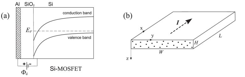
Figure 1: The actual (a) and the model (b) configuration of a 2D conducting system

is of no crucial importance for its principal mission, viz. to confine the electrons along the direction perpendicular to the heterophase boundary. Therefore, to simplify calculations, we hereinafter consider a planar conductor in the form of a rectangular three-dimensional “electron waveguide” with hard side boundaries (Fig. 1b) which envelopes the region

$$x\in(-L/2,L/2)\ ,\qquad y\in[-W/2,W/2]\ ,\qquad z\in[-H/2,H/2]\ .$$ (1)

The length $L$, the width $W$, and the height $H$ of the waveguide will be considered as arbitrary.

According to the linear response theory bib:K57 , the dimensionless (in units of $e^{2}/\pi\hbar$) static conductance $g(L)$ is expressed at $T=0$ in terms of one-particle electron propagators in the following manner,

$$g(L)=\frac{2}{L^{2}}\iint\mathrm{d}\mathbf{r}\,\mathrm{d}\mathbf{r}^{\prime}\frac{\partial}{\partial x}\left[G^{A}(\mathbf{r},\mathbf{r}^{\prime})-G^{R}(\mathbf{r},\mathbf{r}^{\prime})\right]\frac{\partial}{\partial x^{\prime}}\left[G^{A}(\mathbf{r}^{\prime},\mathbf{r})-G^{R}(\mathbf{r}^{\prime},\mathbf{r})\right]\ .$$ (2)

Here, $G^{R,A}(\mathbf{r},\mathbf{r}^{\prime})$ are the retarded (R) and advanced (A) electron Green functions, the integration is taken over the volume occupied by the conductor. Within the isotropic Fermi liquid model and with the units such that $\hbar\bm{=}2m\bm{=}1$ ($m$ is the electron effective mass) the retarded propagator, whose index “R” will be henceforth omitted, is governed by the equation

$$\left[\Delta+k_{F}^{2}+{\rm i}0-V(\mathbf{r})\right]G(\mathbf{r},\mathbf{r}^{\prime})=\delta(\mathbf{r}-\mathbf{r}^{\prime})\ .$$ (3)

Here $\Delta$ is the three-dimensional Laplacian, $k_{F}$ is the Fermi wavenumber, $V(\mathbf{r})$ is the random static potential specified by the zero mean value, $\langle V(\mathbf{r})\rangle=0$, and the binary correlation function $\left<V(\mathbf{r})V(\mathbf{r}^{\prime})\right>=\mathcal{QW}(\mathbf{r}-\mathbf{r}^{\prime})$. We assume the function $\mathcal{W}(\mathbf{r})$ to be normalized to unity and decaying at a characteristic scale $r_{c}$ (the correlation radius). In what follows, for the sake of simplicity, we restrict our consideration to the correlation function of less general form, namely

$$\left<V(\mathbf{r})V(\mathbf{r}^{\prime})\right>=\mathcal{QW}(x-x^{\prime})\delta(\mathbf{r}_{\perp}-\mathbf{r}^{\prime}_{\perp})\ ,\qquad\mathbf{r}_{\perp}=(y,z)\ ,$$ (4)

which evidently should not considerably affect the result.

The equation (3) must be supplemented with proper boundary conditions. The side boundaries of the system, “impenetrable” for electrons, can be characterized by a real impedance which particularly corresponds to the Dirichlet conditions

$$G(\mathbf{r},\mathbf{r}^{\prime})\Bigg{|}_{y=\pm W/2\atop z=\pm H/2}=0\ .$$ (5)

At the same time, the conductor, once attached at the points $x=\pm L/2$ to equilibrium “reservoirs”, should be considered as an open system, which implies two important consequences. First, in Kubo theory the chemical potentials of the massive leads are assumed to be equal to one another. That is why the chemical potential of the junction connecting the leads (or, in the conducting phase, the electron Fermi energy in that junction) can be thought of as being independent of the waveguide geometry, thus allowing to put hereinafter $k_{F}=const$. Second, the openness of the waveguide butt ends imposes the condition for the contact surface impedance to be complex-valued. This results in the differential operation in (3) being non-Hermitian.

In bib:Tar99 ; bib:Tar00 , a method was proposed for solving such a non-Hermitian problem in two dimensions. The analogous procedure is applicable to waveguide-type systems of arbitrary dimensionality as well. The important element of the method is a transition from one originally multi-dimensional stochastic problem to an infinite set of strictly one-dimensional (in general case, non-Hermitian) problems for the propagator $G(\mathbf{r},\mathbf{r}^{\prime})$ mode components. In the next section, the main points of the method bib:Tar99 ; bib:Tar00 are set forth as applied to the system being considered.

III REDUCTION TO ONE DIMENSION

III.1 The general scheme

The suggested algorithm of the multi-dimensional problem (3) reduction to a set of exactly one-dimensional boundary problems is applicable to open systems of arbitrary waveguide configuration at any strength of disorder. The first step consists in proceeding to the mode representation of the electron propagators. In the case of the waveguide depicted in Fig. 1b the transition is carried out by expanding all functions in a whole set of the transverse Laplace operator eigenfunctions, $\bm{|}\mathbf{r}_{\perp};\bm{\mu}\bm{\rangle}$, which are composed of ordinary trigonometric functions. Assuming the boundary conditions (5), these eigenfunctions can be chosen in the form

$$\bm{|}\mathbf{r}_{\perp};\bm{\mu}\bm{\rangle}=\frac{2}{\sqrt{WH}}\sin\left[\left(\frac{y}{W}+\frac{1}{2}\right)\pi n\right]\sin\left[\left(\frac{z}{H}+\frac{1}{2}\right)\pi m\right]\ ,$$ (6)

where $\bm{\mu}=(n,m)$ is the vectorial mode index with the components $n,m\in\aleph$. By the functions (6), the equation (3) is transformed into a set of coupled equations for mode Fourier components of the function $G(\mathbf{r},\mathbf{r}^{\prime})$,

$$\left[\frac{\partial^{2}}{\partial x^{2}}+\kappa^{2}_{\bm{\mu}}+{\rm i}0-V_{\bm{\mu}}(x)\right]G_{\bm{\mu}\bm{\mu}^{\prime}}(x,x^{\prime})-\sum_{\bm{\nu}\neq\bm{\mu}}U_{\bm{\mu}\bm{\nu}}(x)G_{\bm{\nu}\bm{\mu}^{\prime}}(x,x^{\prime})=\delta_{\bm{\mu}\bm{\mu}^{\prime}}\delta(x-x^{\prime})\ .$$ (7)

In (7), the parameter

$$\kappa^{2}_{\bm{\mu}}=k_{F}^{2}-\left({\pi n}/{W}\right)^{2}-\left({\pi m}/{H}\right)^{2}$$ (8)

has the meaning of an unperturbed longitudinal energy of the mode $\bm{\mu}$. The potential matrix $\|U_{\bm{\mu}\bm{\mu}^{\prime}}\|$ is composed of the functions

$$U_{\bm{\mu}\bm{\mu}^{\prime}}(x)=\int_{S}\textrm{d}\mathbf{r}_{\perp}\bm{|}\mathbf{r}_{\perp};\bm{\mu}\bm{\rangle}V(\mathbf{r})\bm{\langle}\mathbf{r}_{\perp};\bm{\mu}^{\prime}\bm{|}$$ (9)

where integration is taken over the conductor cross-section $S$. The diagonal components of this matrix, $V_{\bm{\mu}}(x)\equiv~{}U_{\bm{\mu}\bm{\mu}}(x)$, are responsible for the intra-mode whereas off-diagonal for the inter-mode scattering of quantum particles. In Eq. (7), the term containing the intra-mode potential is deliberately separated from the terms with inter-mode potentials $U_{\bm{\mu}\bm{\nu}}(x)$ ($\bm{\nu}\neq\bm{\mu}$) to avoid singularities in the course of developing the perturbation theory (the proof is presented in Ref. bib:Tar00 ).

The initial problem reformulated in terms of the one-coordinate differential equations (7) cannot actually be considered as strictly one-dimensional due to the entanglement of all mode components of the Green function matrix $\|G_{\bm{\nu}\bm{\mu}}\|$. To reduce equation (3) to a set of independent one-dimensional equations introduce, in the first stage, the auxiliary mode propagators allowing for the scattering by intra-mode potentials only,

$$\left[\frac{\partial^{2}}{\partial x^{2}}+\kappa^{2}_{\bm{\mu}}+{\rm i}0-V_{\bm{\mu}}(x)\right]G^{(V)}_{\bm{\mu}}(x,x^{\prime})=\delta(x-x^{\prime})\ .$$ (10)

For “trial” Green function $G^{(V)}_{\bm{\mu}}(x,x^{\prime})$, the demand of the waveguide openness at the ends $x=\pm L/2$ can be formulated in terms of Sommerfeld’s radiation conditions bib:BF ; bib:V67 . Assuming the contact between the conductor and leads to be ideal (not resulting in scattering), these conditions appear in the form

$$\left(\frac{\partial}{\partial x}\mp{\rm i}\kappa_{\bm{\mu}}\right)G^{(V)}_{\bm{\mu}}(x,x^{\prime})\Bigg{|}_{x=\pm L/2}=0\ ,\qquad\qquad x^{\prime}\in(-L/2,L/2)\ .$$ (11)

Regarding hereinafter the solution of (10), (11) as known precisely, it is worth passing from the differential equation (7) to the integral equation,

$$G_{\bm{\mu}\bm{\mu}^{\prime}}(x,x^{\prime})=G^{(V)}_{\bm{\mu}}(x,x^{\prime})\delta_{\bm{\mu}\bm{\mu}^{\prime}}+\sum_{\bm{\nu}\neq\bm{\mu}}\int_{L}\textrm{d}x_{1}\,\mathsf{R}_{\bm{\mu}\bm{\nu}}(x,x_{1})G_{\bm{\nu}\bm{\mu}^{\prime}}(x_{1},x^{\prime})\ ,$$ (12)

whose kernel,

$$\mathsf{R}_{\bm{\mu}\bm{\nu}}(x,x^{\prime})=G^{(V)}_{\bm{\mu}}(x,x^{\prime})U_{\bm{\mu}\bm{\nu}}(x^{\prime})\ ,$$ (13)

contains the potential $V(\mathbf{r})$ inter-mode harmonics only. From Eq. (12), all of the matrix $\|G_{\bm{\nu}\bm{\mu}}\|$ off-diagonal elements can be expressed in terms of the corresponding diagonal elements by means of some linear operator $\hat{\mathsf{K}}$ specified in coordinate-mode space $\mathsf{M}=\{x,\bm{\nu}\}$,

$$G_{\bm{\nu}\bm{\mu}}(x,x^{\prime})=\int_{L}\mathrm{d}x_{1}\,\mathsf{K}_{\bm{\nu}\bm{\mu}}(x,x_{1})G_{\bm{\mu}\bm{\mu}}(x_{1},x^{\prime})\ ,\qquad\qquad\bm{\nu}\neq\bm{\mu}\ .$$ (14)

The matrix elements of that operator, $\mathsf{K}_{\bm{\nu}\bm{\mu}}(x,x^{\prime})$, satisfy the multi-channel Lippmann-Schwinger equation bib:T75

$$\mathsf{K}_{\bm{\nu}\bm{\mu}}(x,x^{\prime})={\mathsf{R}}_{\bm{\nu}\bm{\mu}}(x,x^{\prime})+\sum_{\bm{\nu}_{1}\neq\bm{\mu}}\int_{L}dx_{1}\,{\mathsf{R}}_{\bm{\nu}\bm{\nu}_{1}}(x,x_{1}){\mathsf{K}}_{\bm{\nu}_{1}\bm{\mu}}(x_{1},x^{\prime})\ ,$$ (15)

whose solution in operator form, $\hat{\mathsf{K}}=(\openone-\hat{\mathsf{R}})^{-1}\hat{\mathsf{R}}$, is expressed in terms of the operator $\hat{\mathsf{R}}$ given in $\mathsf{M}$ by the matrix elements (13).

Note that the lack of the terms with mode index $\bm{\mu}$ in sums of (12) and (15) permits interpreting the operator $\hat{\mathsf{R}}$ as an inter-mode scattering operator acting in the reduced coordinate-mode space ${\mathsf{\overline{M}}_{\bm{\mu}}}$ that includes all the quantum waveguide modes except the mode $\bm{\mu}$. The presence of mode index $\bm{\mu}$ in the kernel of integral operator (14), as well as in other appropriate positions, will be ensured by the projection operator $\bm{P}_{\bm{\mu}}$ that will make the mode index of any operator standing next to it (both from the left and right) equal to the given value $\bm{\mu}$.

By putting $\bm{\mu}^{\prime}=\bm{\mu}$ in Eq. (7) and substituting the inter-mode propagators in the form (14) we eventually arrive at a closed one-dimensional differential equation for the diagonal propagator $G_{\bm{\mu}\bm{\mu}}(x,x^{\prime})$,

$$\left[\frac{\partial^{2}}{\partial x^{2}}+\kappa^{2}_{\bm{\mu}}+{\rm i}0-V_{\bm{\mu}}(x)-\hat{\mathcal{T}}_{\bm{\mu}}\right]G_{\bm{\mu}\bm{\mu}}(x,x^{\prime})=\delta(x-x^{\prime})\ .$$ (16)

Here, along with the “prime” intra-mode potential $V_{\bm{\mu}}(x)$, the effective non-local (operator in $x$-space) potential has arisen,

$$\hat{\mathcal{T}}_{\bm{\mu}}=\bm{P}_{\bm{\mu}}\hat{\mathcal{U}}(\openone-\hat{\mathsf{R}})^{-1}\hat{\mathsf{R}}\bm{P}_{\bm{\mu}}=\bm{P}_{\bm{\mu}}\hat{\mathcal{U}}(\openone-\hat{\mathsf{R}})^{-1}\bm{P}_{\bm{\mu}}\ ,$$ (17)

where $\hat{\mathcal{U}}$ stands for the inter-mode operator potential specified in ${\mathsf{\overline{M}}_{\bm{\mu}}}$ by the matrix elements

$$\bm{|}x,\bm{\mu}\bm{\rangle}\hat{\mathcal{U}}\bm{\langle}x^{\prime},\bm{\nu}\bm{|}=U_{\bm{\mu}\bm{\nu}}(x)\delta(x-x^{\prime})\ .$$ (18)

Strictly speaking, the potential $\hat{\mathcal{T}}_{\bm{\mu}}$, just like $V_{\bm{\mu}}(x)$, is the intra-mode one in that both the initial and the final scattering states belong to the mode $\bm{\mu}$. At the same time, this potential takes exactly into account the inter-mode scattering. From the operator (17) structure it can be seen that the scattering caused by $\hat{\mathcal{T}}_{\bm{\mu}}$ can be regarded as occurring through the intermediate “trial” mode states corresponding to propagators $G^{(V)}_{\bm{\nu}}(x,x^{\prime})$ with $\bm{\nu}\neq\bm{\mu}$. Therefore, the operator $\hat{\mathcal{T}}_{\bm{\mu}}$ will be termed henceforth the inter-mode potential. From the mathematical point of view it is nothing but the conventional T-matrix well known from the quanum theory of scattering bib:N68 ; bib:T75 .

At the final stage of the reduction of the multi-dimensional conductance problem to the one-dimensional problem (16) it is worth representing expression (2) directly through the functions $G_{\bm{\mu}\bm{\mu}}(x,x^{\prime})$. By expanding the electron propagators in terms of eigenfunctions (6) one can discriminate two different terms of the conductance. Within the first term, henceforth conditionally called the “diagonal” conductance, $g^{(d)}(L)$, we collect those expansion terms which from the outset contain the diagonal mode propagators $G_{\bm{\mu}\bm{\mu}}$. All the other expansion terms, containing mode components $G_{\bm{\nu}\bm{\mu}}$ with $\bm{\nu}\neq\bm{\mu}$, will be gathered in the second term, the “non-diagonal” conductance $g^{(nd)}(L)$. Taking into account the relationship (14) and the fact that both the retarded and advanced Green functions of the evanescent modes ($\kappa^{2}_{\bm{\mu}}<0$) at weak scattering can be regarded as real-valued (see Eq. (23) in the next subsection) the above-indicated terms of the conductance can be represented as

$$g^{(d)}(L)=-\frac{4}{L^{2}}\overline{\sum_{\bm{\mu}}}\iint_{L}\mathrm{d}x\,\mathrm{d}x^{\prime}\frac{\partial G_{\bm{\mu}\bm{\mu}}(x,x^{\prime})}{\partial x}\frac{\partial G_{\bm{\mu}\bm{\mu}}^{*}(x,x^{\prime})}{\partial x^{\prime}}\ ,$$ (19a)

$$g^{(nd)}(L)=-\frac{4}{L^{2}}\overline{\sum_{\bm{\mu},\bm{\nu}\atop\bm{\nu}\neq\bm{\mu}}}\iiiint_{L}\mathrm{d}x_{1}\ldots\mathrm{d}x_{4}\,\frac{\partial{\sf K}_{\bm{\nu}\bm{\mu}}(x_{1},x_{2})}{\partial x_{1}}G_{\bm{\mu}\bm{\mu}}(x_{2},x_{4}){\sf K}_{\bm{\nu}\bm{\mu}}^{*}(x_{1},x_{3})\frac{\partial G_{\bm{\mu}\bm{\mu}}^{*}(x_{3},x_{4})}{\partial x_{4}}\ .$$ (19b)

The bar over the sum symbols in (19) indicates the summation over extended modes only, i.e. the modes with mode energies $\kappa^{2}_{\bm{\mu}}>0$.

III.2 The weak scattering approximation

In view of statistical formulation of the problem, the important ingredient of the calculation technique, viz., the trial Green function $G^{(V)}_{\bm{\mu}}(x,x^{\prime})$, can be thought of as known precisely if one manages to find all its statistical moments $\langle\big{[}G^{(V)}_{\bm{\mu}}(x,x^{\prime})\big{]}^{p}\rangle$, $p\in\aleph$. In the case of a strongly disordered system this can certainly be done with the aid of numerical methods only. Yet provided the scattering from the potential $V(\mathbf{r})$ is regarded as weak, these moments can be obtained analytically using, e.g., the method of bib:Tar00 which takes properly into account the multiple scattering in the stochastic problem (10), (11).

The weakness criteria can be formulated in terms of the inequalities

$$k_{F},\,r_{c}\ll\ell\ ,$$ (20)

where $\ell$ stands for the quasi-classical mean free path of conducting electrons. In the particular case of a white-noise-type potential, i.e. at $\mathcal{W}(x)=\delta(x)$ in (4), this length equals to $4\pi/\mathcal{Q}$. Subject to conditions (20), calculation of the required moments for the case of extended modes yields

$$\Big{<}\left[G^{(V)}_{\bm{\mu}}(x,x^{\prime})\right]^{p}\Big{>}=\left(\frac{-\mathrm{i}}{2\kappa_{\bm{\mu}}}\right)^{p}\exp\Bigg{[}\mathrm{i}p\kappa_{\bm{\mu}}|x-x^{\prime}|-\frac{p}{2}\left(\frac{p}{L_{f}^{(V)}(\bm{\mu})}+\frac{1}{L_{b}^{(V)}(\bm{\mu})}\right)|x-x^{\prime}|\Bigg{]}\ .$$ (21)

Here, $L_{f,b}^{(V)}(\bm{\mu})$ are the forward ($f$) and backward ($b$) scattering lengths of the mode $\bm{\mu}$ which are associated with the prime intra-mode potential $V_{\bm{\mu}}(x)$,

$$L_{f}^{(V)}(\bm{\mu})=\frac{4S}{9\mathcal{Q}}\left(2\kappa_{\bm{\mu}}\right)^{2}\ ,\hskip 42.67912ptL_{b}^{(V)}(\bm{\mu})=\frac{4S}{9\mathcal{Q}}\frac{\left(2\kappa_{\bm{\mu}}\right)^{2}}{\widetilde{\mathcal{W}}(\kappa_{\bm{\mu}})}\ ,$$ (22)

$\widetilde{\mathcal{W}}(\kappa_{\bm{\mu}})$ is the Fourier transform of $\mathcal{W}(x)$. As far as the evanescent modes are concerned, at weak scattering (WS) the potential $V_{\bm{\mu}}(x)$ can be omitted from (10), thus allowing one to take advantage of the unperturbed solution,

$$G^{(V)}_{\bm{\mu}}(x,x^{\prime})=-\frac{1}{2|\kappa_{\bm{\mu}|}}\exp\big{(}-|\kappa_{\bm{\mu}}||x-x^{\prime}|\big{)}\ .$$ (23)

The functional structure of $T$-matrix (17) and, consequently, of equation (16) is substantially simplified with the proviso (20). Direct estimation, with the use of (13) and (21), of the operator $\hat{\mathsf{R}}$ norm in the space of reference functions $\{\exp(\mathrm{i}\kappa_{\bm{\mu}}x)\}$ is written as

$$\|\hat{\mathsf{R}}\|^{2}\sim\frac{1}{\kappa_{\bm{\mu}}\ell}\ .$$ (24)

This enables us to replace the exact operator $\hat{\mathsf{K}}$, specified by equation (15), with its approximate value $\hat{\mathsf{K}}\approx\hat{\mathsf{R}}$. As a result, the potential (17) assumes the form

$$\hat{\mathcal{T}}_{\bm{\mu}}=\bm{P}_{\bm{\mu}}\hat{\mathcal{U}}\hat{\mathcal{G}}^{(V)}\hat{\mathcal{U}}\bm{P}_{\bm{\mu}}\ ,$$ (25)

where the operator $\hat{\mathcal{G}}^{(V)}$ is specified on ${\mathsf{\overline{M}}_{\bm{\mu}}}$ by matrix elements

$$\bm{|}x,\bm{\nu}\bm{\rangle}\hat{\mathcal{G}}^{(V)}\bm{\langle}x^{\prime},\bm{\nu}^{\prime}\bm{|}=G^{(V)}_{\bm{\nu}}(x,x^{\prime})\delta_{\bm{\nu}\bm{\nu}^{\prime}}\ .$$ (26)

The analogous substitution of the operator $\hat{\mathsf{K}}$ approximate matrix elements into Eq. (19b) allows one to conclude that at weak scattering the non-diagonal part of the conductance is parametrically small as compared to its diagonal counterpart. This is also confirmed by numerical calculation of both of the conductance terms. Considering this fact, we further restrict ourselves to the analysis of the term (19a) only, assuming that $g(L)\approx g^{(d)}(L)$.

IV Analysis of the mode states spectrum

Unlike the original potential $V(\mathbf{r})$ and, accordingly, its mode matrix elements in equation (7) the effective potential $\hat{\mathcal{T}}_{\bm{\mu}}$ has a non-zero mean value. In what follows, to apply the perturbation theory in this potential one has to separate its averaged and fluctuating parts, $\langle\hat{\mathcal{T}}_{\bm{\mu}}\rangle$ and $\Delta\hat{\mathcal{T}}_{\bm{\mu}}=\hat{\mathcal{T}}_{\bm{\mu}}-\langle\hat{\mathcal{T}}_{\bm{\mu}}\rangle$. As a basic approximation for mode propagator $G_{\bm{\mu}\bm{\mu}}(x,x^{\prime})$ consider the Green function of the equation

$$\left[\frac{\partial^{2}}{\partial x^{2}}+\kappa^{2}_{\bm{\mu}}+{\rm i}0-\langle\hat{\mathcal{T}}_{\bm{\mu}}\rangle\right]G^{(0)}_{\bm{\mu}\bm{\mu}}(x,x^{\prime})=\delta(x-x^{\prime})\ ,$$ (27)

which differs from (16) by the lack of the fluctuating potentials. On defining the operator $\langle\hat{\mathcal{T}}_{\bm{\mu}}\rangle$ action onto the function $G^{(0)}_{\bm{\mu}\bm{\mu}}(x,x^{\prime})$ it is important to notice that there is no correlation between inter- and intra-mode scattering in the waveguide with hard side boundaries, viz. the equality holds

$$\left<U_{\bm{\mu}\bm{\nu}}(x)V_{\bm{\nu}}(x^{\prime})\right>=0\ .$$ (28)

Owing to this, the potential (25), subject to configurational averaging, is transformed from a non-local operator to a multiplicative constant. It was shown in bib:Tar00 that its effect on the mode energy $\kappa^{2}_{\bm{\mu}}$ is reduced to occurrence of the mode self-energy $\Sigma(\kappa_{\bm{\mu}})=\Delta\kappa_{\bm{\mu}}^{2}+\mathrm{i}/\tau_{\bm{\mu}}^{(\varphi)}$,

$$\left(\langle\hat{\mathcal{T}}_{\bm{\mu}}\rangle\hat{G}^{(0)}_{\bm{\mu}\bm{\mu}}\right)(x,x^{\prime})=-\Sigma(\kappa_{\bm{\mu}})G^{(0)}_{\bm{\mu}\bm{\mu}}(x,x^{\prime})\ .$$ (29)

By reproducing the calculation procedure given in bib:Tar00 with reference to the system discussed in this paper one can obtain

$$\Delta\kappa_{\bm{\mu}}^{2} = \frac{\mathcal{Q}}{S}\sum_{\bm{\nu}\neq\bm{\mu}}\mathcal{P}\int_{-\infty}^{\infty}\frac{\mathrm{d}q}{2\pi}\;\frac{\widetilde{\mathcal{W}}(q+\kappa_{\bm{\mu}})}{q^{2}-\kappa_{\bm{\nu}}^{2}}\ ,$$ (30a)

$$\frac{1}{\tau_{\bm{\mu}}^{(\varphi)}} = \frac{\mathcal{Q}}{4S}\overline{\sum_{\bm{\nu}\neq\bm{\mu}}}\frac{1}{\kappa_{\bm{\nu}}}\left[\widetilde{\mathcal{W}}(\kappa_{\bm{\mu}}-\kappa_{\bm{\nu}})+\widetilde{\mathcal{W}}(\kappa_{\bm{\mu}}+\kappa_{\bm{\nu}})\right]\ .$$ (30b)

In (30a), the symbol $\mathcal{P}$ stands for the integral principal value.

The absolute value of the self energy (30) prove to be not rather sensitive to the number of open channels. At any $N_{c}>1$ the estimate $\Delta\kappa_{\bm{\mu}}^{2}\sim 1/\tau_{\bm{\mu}}^{(\varphi)}\sim k_{F}/\ell$ holds, which nearly for all modes allows disregarding the mode energy renormalization given by the term (30a). At the same time, the mode level uncertainty, (30b), is of crucial importance for further analysis of the electron dynamics. The level width, apart from being finite in magnitude, is quick to saturate with a growth in the number of open channels. Specifically, within the model of point-like scatterers the asymptotic of the term (30b) at $N_{c}\gg 1$ reads

$$\frac{1}{\tau_{\bm{\mu}}^{(\varphi)}}\approx\frac{\mathcal{Q}k_{F}}{4\pi}=\frac{k_{F}}{\ell}\ .$$ (31)

Note particularly that in (30b), as opposed to (30a), the summation is carried out over extended modes only of the quantum waveguide, the mode $\bm{\mu}$ itself being excluded as an intermediate state. In the case of a single-channel conductor, where solely the lowest mode $\bm{\mu}_{1}=(1,1)$ is non-local, the self energy is free of the term (30b).

The imaginary part of self energy (30) can be interpreted as an effect of the coherent mode state dephasing. From expression (30b) structure it follows that for any given mode $\bm{\mu}$ the re-entrant electron scattering through the non-local intermediate modes, with the proviso that the latter are present in the system at hand, serves as a cause of dephasing. This suggests the interpretation that for any current-carrying mode in the conductor all other extended modes, except the mode $\bm{\mu}$ itself, can be thought of as a peculiar “dephasing environment”. Interaction of modes with this environment is realized via the inter-mode scattering from the potential $V(\mathbf{r})$. Although the scattering from static disorder is certainly elastic in terms of a one-electron energy (at $T=0$ the latter remains Fermian), the many-particle mode states are specified by distinct (longitudinal) energies. This suggests considering the virtual inter-mode transitions, “hidden” in $T$-matrices (17) and (25), as being effectively inelastic, thereby making it possible to adhere to the conventional point of view which does associate the dephasing of quantum states solely with inelastic processes.

Note that the inter-mode scattering via solely strongly localized evanescent modes (single-mode conductor) does not result in dephasing the mode states. The dephasing effect is noticeable provided electrons are scattered through essentially non-local extended modes, which is certainly possible if there are at least two such modes in the conductor. This leads us to conclude that the preservation of quantum states spatial coherence is every bit as important for interferential Anderson localization as the time coherence.

The effect of fluctuating potentials, $V_{\bm{\mu}}(x)$ and $\Delta\hat{\mathcal{T}}_{\bm{\mu}}$, can be analyzed by evaluating the corresponding Born scattering rates, $1/\tau_{\bm{\mu}}^{(V)}$ and $1/\tau_{\bm{\mu}}^{(\mathcal{T})}$. Taking into account the operator (25) structure and the estimate (31) one can readily obtain

$$\frac{\tau_{\bm{\mu}}^{(\varphi)}}{\tau_{\bm{\mu}}^{(V)}} \sim \left[k_{F}r_{c}N_{c}\cos^{2}\vartheta_{\bm{\mu}}\right]^{-1}\ ,$$ (32a)

$$\frac{\tau_{\bm{\mu}}^{(\varphi)}}{\tau_{\bm{\mu}}^{(\mathcal{T})}} \sim \frac{\tau_{\bm{\mu}}^{(\varphi)}}{\tau_{\bm{\mu}}^{(V)}}\times\left\{\begin{array}[]{ccc}L/\ell&,&\qquad L<\ell\\ N_{loc}^{(s)}&,&\qquad L>\ell\end{array}\right.\ .$$ (32d)

Here, $\vartheta_{\bm{\mu}}$ is the mode $\bm{\mu}$ angle of slide ($\cos\vartheta_{\bm{\mu}}=|\kappa_{\bm{\mu}}|/k_{F}$), $N_{loc}^{(s)}\leq N_{c}$ is the number of trial mode states corresponding to equation (10), whose localization lengths, $4L_{b}^{(V)}(\bm{\mu})$, do not exceed the conductor length $L$.

Since in real materials the condition $k_{F}r_{c}\gtrsim 1$ normally holds, it is easy to make sure that the potential $V_{\bm{\mu}}(x)$ has a negligible effect on the electron dynamics in multi-mode systems. The same applies to the potential $\Delta\hat{\mathcal{T}}_{\bm{\mu}}$ if one assumes the conductor length $L\ll N_{c}\ell$. The comprehensive analysis performed in bib:Tar00 has revealed that the scattering on this potential (substantially non-local in the case of $N_{c}>1$) does not either affect the conductance significantly if $L\gg N_{c}\ell$. This seems to be quite natural if one bears in mind that the potential $\Delta\hat{\mathcal{T}}_{\bm{\mu}}$ brings about the re-entrant scattering. From the standpoint of perturbation theory this implies that in scattering from the potential $\Delta\hat{\mathcal{T}}_{\bm{\mu}}$ the inter-mode potentials $U_{\bm{\mu}\bm{\nu}}(x)$ contribute twice as much as they do when self energy (30) is obtained.

Turning back to the prime intra-mode potential $V_{\bm{\mu}}(x)$, it should be stressed that, subject to the condition (20), the mode states spatial coherence is slightly violated by scattering on this potential. In multi-mode conductors ($N_{c}\gg 1$) this scattering leads to weak localization corrections to the conductance, which are not dealt with in this paper. Clearly, the role of those corrections increases with a decreasing number of conducting channels, but they do not considerably affect the result obtained within the kinetic approach even at $N_{c}\sim 1$. The potential $V_{\bm{\mu}}(x)$ is determining for the electron spectrum in one-dimensional conductors only, which will be discussed in more details in the next section.

V The conductance dependence on the conductor configuration

The mode state spectrum is governed, along with the electron energy, by the confinement potential configuration, i.e. by the conductor geometry, according to the model being considered. While the bulk wire conductance changes, with a variation of the conductor shape, in compliance with the conventional Ohm’s law, in the case where at least one of the conductor dimensions is comparable to microscopic length scales pertinent to the system at hand the quantization becomes extremely important. Consider some limiting cases where the dimensional quantization affects the electron dynamics quite differently.

V.1 Multi-mode conductors

If the confinement potential and the electron energy are such that there is more than one conducting channel in the quantum waveguide, the exact Green function $G_{\bm{\mu}\bm{\mu}}(x,x^{\prime})$ can be shown, including (32), to be well-approximated in the range $L\ll N_{c}\ell$ by the function $G^{(0)}_{\bm{\mu}\bm{\mu}}(x,x^{\prime})$. In the region $L>N_{c}\ell$ the replacement of the exact propagator in (19a) by its approximate form from equation (27) is yet justified in view of statistical averaging over the disorder. The solution of (27) which meets the radiation conditions at open ends of the conductor has the form

$$G_{\bm{\mu}\bm{\mu}}^{(0)}(x,x^{\prime})=\frac{1}{2\mathrm{i}\kappa_{\bm{\mu}}}\exp\Big{\{}\big{[}\mathrm{i}\kappa_{\bm{\mu}}-1/l_{\bm{\mu}}^{(\varphi)}\big{]}|x-x^{\prime}|\Big{\}}\ .$$ (33)

Here, $l_{\bm{\mu}}^{(\varphi)}=2\kappa_{\bm{\mu}}\tau_{\bm{\mu}}^{(\varphi)}$ is the mode $\bm{\mu}$ extinction length (or, equivalently, its dephasing length) associated with the incoherent inter-mode scattering. Substitution of (33) into (19a) results in the average conductance expression as follows,

$$\big{<}g(L)\big{>}=\overline{\sum_{\bm{\mu}}}\frac{l_{\bm{\mu}}^{(\varphi)}}{L}\left[1-\frac{l_{\bm{\mu}}^{(\varphi)}}{L}\exp\left(-\frac{L}{l_{\bm{\mu}}^{(\varphi)}}\right)\sinh\frac{L}{l_{\bm{\mu}}^{(\varphi)}}\right]\ .$$ (34)

If the number of channels is large, $N_{c}\gg 1$, the replacement of the sum (34) by the integral results in simple limiting formulas valid in the regions corresponding to classically ballistic ($L\ll\ell$) and diffusive ($L\gg\ell$) electron transport, namely

$$\big{<}g(L)\big{>}\approx N_{c}\qquad\ ,\hskip 28.45274ptL\ll\ell\ ,$$ (35a)

$$\big{<}g(L)\big{>}\approx\frac{4}{3}\frac{N_{c}\ell}{L}\quad,\hskip 28.45274ptL\gg\ell\ .$$ (35b)

In the ballistic limit (35a), the conductance as a function of the electron energy or the confinement potential has a staircase-like structure with the step height being equal exactly to the conductance quantum $G_{0}=e^{2}/\pi\hbar$ (recall that for a massive tree-dimensional wire the equality $N_{c}=[k_{F}^{2}S/4\pi]$ holds, where $[...]$ stands for the integer part of the number enclosed). As the electron motion changes from ballistic to diffusive regime, the conductance approaches asymptotically the classical value (35b) well known from the kinetic theory. Staircase structure of the conductance is formally kept safe, but the step height is decreased in proportion to the ratio $\ell/L$. The conductance dependence on the quantum waveguide length is displayed in Fig. 2. The curves correspond to different numbers of open channels. Nevertheless, all of them show the same “ohmic” behaviour at lengths obeying $L/\ell>1$.

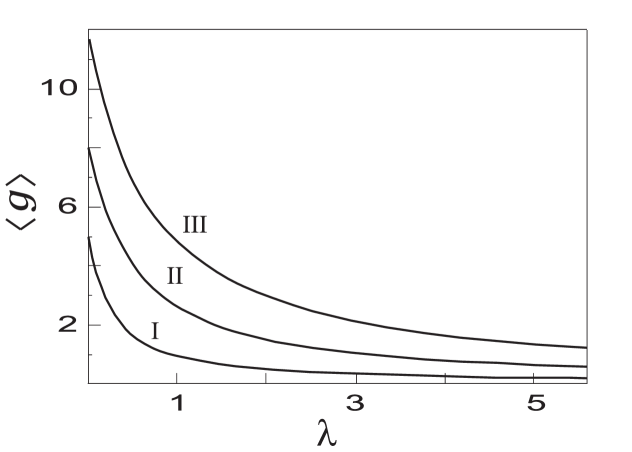
Figure 2: The conductance (34) as a function of the dimensionless length $\lambda=L/\ell$ for conductors with different number of open channels: I — $N_{c}=5$, II — $N_{c}=8$, III — $N_{c}=12$.

V.2 Anderson localization in a single-mode conductor

If the electron system parameters permit one open channel only, all other modes of the quantum waveguide are inhomogeneous, strongly localized along the $x$ coordinate (so-called evanescent modes). In this case the potential $\hat{\mathcal{T}}_{\bm{\mu}}$, as well as $V_{\bm{\mu}}(x)$, is real-valued and local. Therefore, the perturbation theory in the form used above ceases to be practical since the weak scattering, including the inter-mode one, does not substantially violate the coherence of each extended mode. Calculation of the conductance in this case calls for a method which would take into account the interference of multiply scattered quantum waves, e.g., the methods used in bib:B73 ; bib:AR78 to obtain the conductivity of 1D disordered conductors.

In bib:MT98 ; bib:MT01 , with the use of the resonance weak scattering method equivalent to those of bib:B73 ; bib:AR78 , the general expression for the entire set of statistical moments of the single-mode wire conductance was obtained in the case of the disorder produced by side boundary roughness of the conductor instead of its bulk inhomogeneities. Technically, the rough-boundary problem is identical to that considered in this paper, so application of the method bib:MT98 ; bib:MT01 to a single-mode bulk-disordered conductor yields

$$\big{<}g^{n}(L)\big{>} = \frac{4}{\sqrt{\pi}}\left[\frac{L_{b}^{(V)}(\bm{\mu}_{1})}{L}\right]^{3/2}\exp{\left[-\frac{L}{4L_{b}^{(V)}(\bm{\mu}_{1})}\right]}\int_{0}^{\infty}\frac{zdz}{\cosh^{2n-1}z}\exp\left[-z^{2}\frac{L_{b}^{(V)}(\bm{\mu}_{1})}{L}\right]\int_{0}^{z}dy\,\cosh^{2(n-1)}y\,,\qquad$$ (36)

$$n = 0,\pm 1,\pm 2,\ldots\ .$$

It can be concluded from (36) that in the one-channel case two regimes only of the electron transport can be distinguished, viz. “ballistic” and “localized”, the corresponding limiting expressions for the average conductance being

$$\langle g(L)\rangle\approx\begin{cases}1-4L/\xi_{1}\ ,&\qquad L/\xi_{1}\ll 1\\ (\pi^{5/2}/16)\left(\xi_{1}/L\right)^{3/2}\exp\left(-L/\xi_{1}\right)\ ,&\qquad L/\xi_{1}\gg 1\end{cases}\ .$$ (37)

Here, $\xi_{1}=4L_{b}^{(V)}(\bm{\mu_{1}})$ is the harmonics $\bm{\mu}_{1}$ one-dimensional localization length associated with the electron backscattering on the prime intra-mode potential $V_{\bm{\mu}_{1}}(x)$.

V.3 Metal-insulator transition as a quantum phase transition

The conductance (37) evidently exhibits the localized character of the electron transport in a single mode quantum waveguide, in accordance with the well-known results of 1D disordered system spectral analysis bib:LGP82 . This fact in itself suggests that it is in principle possible for the finite electron system to be transferred from conducting to insulating state subject to the geometrical factors only, the disorder being kept constant. The one-dimensional Anderson-type localization is known to be universal in linear systems, in that all the electron states in 1D random potential are localized in infinite-length systems, irrespective of the electron energy. At the same time, this localization, in a sense, can be considered to be weak. On lowering the disorder level the length $\xi_{1}$ increases infinitely, so that in relatively perfect conductors, their length being even extremely large, the collective motion of the electrons can actually remain nearly ballistic.

The approach suggested in this paper provides an explanation for the observed MIT even at moderate, viz., mesoscopic, sample lengths, the disorder being arbitrary enough. When decreasing the cross-section area, the conductor should ultimately turn to a below-cut-off waveguide regime where all of the modes become evanescent, each being localized at a scale of the wavelength $|\kappa_{\bm{\mu}}|^{-1}$ which, in the context of calculation technique being used, is considered as microscopic. In such a “dimensionally localized” regime, the conductance falls sharply with respect to its value (37) in the “marginal” one-mode state, thus allowing for being regarded as equal to zero with parametric accuracy.

It is essential that the mode spectrum of the conductor depicted in Fig. 1b can be varied by changing just one of its transverse dimensions, the other being kept constant. From (8) it can be seen that even at large enough width $W$ the quantum waveguide can be carried over to the below-cut-off regime subject to the decrease of its thickness $H$ only. In real planar systems this is achieved by either increasing the depletion voltage (see Fig. 1a) or by acting upon the heterocontact region capacitively.

In Fig. 3, the numerical data are presented showing the conductance (34) dependence on the conductor thickness, the width being fixed. The curve I conforms to the ballistic limit $\ell/L\to\infty$, whereas the curves II and III to the finite values of this ratio. The ballistic conductance is ideally quantized, each step being equal to the quantum $G_{0}$. The peculiar slow modulation of the curves is due to the waveguide model used, Fig. 1b, whose spectrum requires the opening or closing of the conducting channels to occur non-equidistantly in the value of $H$.

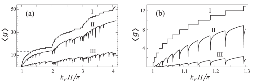
Figure 3: The dimensionless conductance vs the quantum waveguide thickness, at fixed width ($k_{F}W/\pi=~{}20.5$) and different values of the diffusion parameter $\lambda=L/\ell$. The curve I corresponds to $\lambda=0$, II to $\lambda=0,5$, III to $\lambda=5$.

As the disorder increases (the curves II and III), the conductance steps become lower, their contours being smoothed out. In the vicinity of the channel opening (closing) points significant dips in the conductance should be observed. The shape of the dips can be clearly seen in Fig. 3b, where the region separated in Fig. 3a is shown at the expanded scale. When approaching the channel closing point from the large $H$ side, the conductance slowly decreases. This takes place due to the increase in the density of states of the slow marginal mode $\bm{\mu}_{m}$ and, consequently, due to the electron transfer to this mode from more “fast” open channels. The dephasing rates of the latter, Eq. (30b), have square-root singularities at the critical points, which results in the destructive reduction of the mode propagator (33) when approaching the point corresponding to $\kappa_{\bm{\mu}_{m}}=0$.

The analogous dips were found in the waveguide system optical conductance calculated numerically using the Landauer approach bib:GSGC96 . However, in bib:GSGC96 the dips were relatively symmetric with respect to the points of extended mode disappearance, whereas in Fig. 3 they appear to be pronouncedly asymmetric in form. The skewness is explained by the fact that in deriving the expression (34) in the WS approximation we have disregarded the evanescent mode contribution to the conductance, thus omitting the tunnel part of the conductance which is governed by those modes. This is not quite justified for marginal modes since the WS condition for them is violated at the critical point, so that just after the mode closing its propagator does not equal exactly to (23).

The graphs in Fig. 3 display a succession of quantum phase transitions which take place in the electron system if one changes the confinement potential. At the critical points the conductance varies stepwise, the marginal mode wavelength serving as a correlation length in the electron system.

The leftmost phase transition, clearly seen in Fig. 3b, can be interpreted as the electron system transition from metallic to dielectric state. In the metallic phase, straight to the right of the transition point, the conductance in the ideal ballistic situation equals exactly to the quantum $G_{0}$. This is in a good agreement with the resistance values observed alongside the so-called separatrix, the conventional line separating the ensembles of experimental curves showing the resistance temperature dependence in dielectric and conducting phases of two-dimensional systems bib:AKS01 .

In most of the experimental works the 2D systems spectral classification is performed on the bases of the temperature and the magnetic field dependence of their resistance. The detailed analysis of the magnetic-field-induced effects is beyond the scope of this paper. As far as the resistance temperature dependence is concerned, some qualitative conclusions can be made in accordance with the above described peculiarities of the quantum transport in planar systems.

It should be noted that the transition from the metallic-type conductance (34), (35) to its small value in the localized ($0$-mode) phase proceeds inevitably through the one-mode state of the electron system, the latter behaving like the effectively one-dimensional in spite of the macroscopic width. It has already been predicted, in bib:AR78 for the case of $T\tau>>1$ and in bib:T92 for $T\tau<<1$, that a 1D system conductivity should exhibit non-monotonic dependence on $T$. And in fact, the actual 2D system resistance measured on the metallic side close to the separatrix tends to change non-monotonically with temperature bib:AKS01 .

The weak temperature dependence of the separatrix itself can also be explained if one takes into account that the mode wavelength of the last-remaining extended mode grows infinitely as far as one approaches its closing point. Since this length prove to exceed ultimately the wavelength of thermal phonons, the interaction between the marginal-mode electrons, whose density of states grows proportionally to the mode wavelength, turns out to be ineffective.

In conclusion, deep in the dielectric phase, where all the electron modes become evanescent, that is, strongly localized in the direction of current, it is natural to anticipate the resistance temperature dependence predicted by the percolation theory bib:SE79 . The dependence similar to this type is widely observed in real two-dimensional systems far in the dielectric side from the separatrix bib:AKS01 ; bib:MKBF95 .

VI Concluding remarks

The objective of the present paper was to elaborate a one-particle field model of a 2D electron system transition from the dielectric state suggested by the scaling theory of localization to a metallic phase widely observed in experiment. The essence of the proposed approach lies in the fact that electrons (or holes), being experimentally regarded as evidently two-dimensional, should be really believed to be propagating in a virtual three-dimensional quantum waveguide formed by the confinement potential. Within the framework of this approach, the quantum nature of the electrons can be fully taken into account.

Note that the technique of a multi-dimensional problem reduction to a set of strictly one-dimensional problems, which is the key point of the suggested analytical procedure, is also applicable to those systems which are initially considered as strictly two-dimensional ones bib:Tar99 ; bib:Tar00 . However, the possibility for such systems to change from the metallic to dielectric state can hardly be noticed within the framework of this technique. The point is that even a single-mode state of a 2D electron system, let alone its $0$-mode regime, is generally associated not with a macroscopic conductor but rather with an extremely narrow strip-like quantum wire.

In spite of such a perception, a macroscopic two-dimensional quantum waveguide, being actually considered as a flattened three-dimensional one, can be easily reduced to the single-mode and then even to the below-cut-off ($0$-mode) state. Thereupon, the question is bound to arise which electron systems can be reasonably attributed to a class of two-dimensional systems and which cannot be. Moreover, is there, in fact, the essential difference, from the transport properties standpoint, between any non-one-dimensional electron systems and three-dimensional ones?

It is difficult to ascertain the objective criteria for distinguishing between 2D and 3D electron systems based solely on the results given in this paper. The point is that only the diffusion-type conductance typical for non-single-mode real disordered systems and the “localized” conductance pertinent to one-mode conducting as well as $0$-mode (dielectric) systems seem to be fundamentally different. Additionally, if one considers that 2D and 3D transport problems in the mode representation are similarly reduced to one-dimensional ones, the conclusion suggests itself that it might be logical to classify the non-ballistic systems of Fermian type in terms of the mode content instead of their formal geometrical structure. From this standpoint, two kinds of systems seem to be, in actual fact, fundamentally different, viz. systems possessing more than one extended mode (both two- and three-dimensional), wherein the diffusive quasi-particle transport is realized, and those which can be conditionally referred to as the “localized” systems. The latter class includes one-mode systems subject to Anderson-type localization (weak or strong, depending on the disorder strength) and $0$-mode systems in which the localization is merely related to the dimensional quantization of the electron spectrum rather than to the disorder and/or Coulomb interaction of carriers.

References

- (1) E. Abrahams, S. V. Kravchenko, and M. P. Sarachik, Rev. Mod. Phys. 73, 251 (2001).
- (2) E. Abrahams, P. W. Anderson, D. C. Licciardello, and T. V. Ramakrishnan, Phys. Rev. Lett. 42, 673 (1979).
- (3) A. M. Finkel’stein, Z. Phys. B 56, 189 (1984).
- (4) C. Castellani, C. D. Di Castro, and P. A. Lee, Phys. Rev. B 57, R9381 (1998).
- (5) S. Chakravarty, L. Yin, and E. Abrahams, Phys. Rev. B 58, R559 (1998).
- (6) D. Belitz and T. R. Kirkpatrick, Phys. Rev. B 58, 8214 (1998).
- (7) J. S. Takur and D. Neilson, Phys. Rev. B 58, 13717 (1998).
- (8) T. M. Klapwijk and S. Das Sarma, Solid State Commun. 110, 581 (1999).
- (9) S. Das Sarma and E. H. Hwang, Phys. Rev. Lett. 84, 5596 (2000).
- (10) S. L. Sondhi, S. M. Girvin, J. P. Carini, and D. Shahar, Rev. Mod. Phys. 69, 315 (1997).
- (11) P. A. Lee and T. V. Ramakrishnan, Rev. Mod. Phys. 57, 287 (1985).
- (12) P. Mohanty, Physica B 280, 446 (2000); idem, cond-mat/9912263.
- (13) I. L. Aleiner, B. L. Altshuler, and M. E. Gershenson, Waves Random Media 9, 201 (1999).
- (14) B. L. Altshuler, A. G. Aronov, and P. A. Lee, Phys. Rev. Lett. 44, 1288 (1980).
- (15) B. Tanatar and D. M. Ceperley, Phys. Rev. B 39, 5005 (1989).
- (16) D. Belitz and T. R. Kirkpatrick, Rev. Mod. Phys. 66, 261 (1994).
- (17) Yu. V. Tarasov, J. Phys.: Condens. Matter 11, L437 (1999).
- (18) Yu. V. Tarasov, Waves Random Media 10, 395 (2000).
- (19) F. Mancini and A. Avella, cond-mat/0006377.
- (20) K. B. Efetov, Adv. Phys. 32, 53 (1983).
- (21) O. N. Dorokhov, Solid State Commun. 51, 381 (1984).
- (22) P. A. Mello, P. Pereyra, and N. Kumar., Ann. Phys., 181, 290 (1988).
- (23) M. P. Sarachik and S. V. Kravchenko, Proc. Natl. Acad. Sci. USA 96, 5900 (1999); idem, cond-mat/9903292.
- (24) R. Kubo, J. Phys. Soc. Jpn. 12, 570 (1957).
- (25) F. G. Bass and I. M. Fuks, Wave Scattering from Statistically Rough Surfaces (Pergamon, New York, 1979).
- (26) V. S. Vladimirov, Equations of mathematical physics (Moscow: Nauka, 1967) (in Russian).
- (27) J. R. Taylor, Scattering Theory. The Quantum Theory on Nonrelativistic Collisions (New York: Wiley, 1972).
- (28) R. Newton. Scattering Theory of Waves and Particles (New York: McGraw-Hill, 1968).
- (29) V. L. Berezinski, Zh. Eksp. Teor. Fiz. 65, 1251 (1973) [Sov. Phys.-JETP 38, 620 (1974)].
- (30) A. A. Abrikosov and I. A. Ryzhkin, Adv. Phys. 27, 147 (1978).
- (31) N. M. Makarov and Yu. V. Tarasov, J. Phys.: Condens. Matter 10, 1523 (1998).
- (32) N. M. Makarov and Yu. V. Tarasov, Phys. Rev. B64, 235306 (2001).
- (33) I. M. Lifshits, S. A. Gredeskul and L. A. Pastur, Introduction to the Theory of Disordered Systems (Wiley, New York, 1988).
- (34) P. García-Mochales, P. Serena, N. García, and J. L. Costa-Krämer, Phys. Rev. B53, 10268 (1996).
- (35) Yu. V. Tarasov, Phys. Rev. B 45, 8873 (1992).
- (36) B. I. Shklovskii and A. L. Efros, Electronic Properties of Doped Semiconductors (Nauka, Moscow, 1979) (in Russian).
- (37) W. Mason, S. V. Kravchenko, G. E. Bowker, and J. E. Furneaux, Phys. Rev. B52, 7857 (1995).