Towards a Non-extensive Random Matrix Theory.

Abstract

In this article the statistical properties of symmetrical random matrices whose elements are drawn from a $q$-parametrized non-extensive statistics power-law distribution are investigated. In the limit as $q\rightarrow 1$ the well known Gaussian orthogonal ensemble (GOE) results are recovered. The relevant level spacing distribution is derived and one obtains a suitably generalized non-extensive Wigner distribution which depends on the value of the tunable non-extensivity parameter $q$. This non-extensive Wigner distribution can be seen to be a one-parameter level-spacing distribution that allows one to interpolate between chaotic and nearly integrable regimes.

The Hamiltonian $M\times M$ matrix that is examined is symmetric and real. In order to simplify the derivation $M$ is restricted to $M=2$. The derivation of the $2\times 2$ random matrix statistics follows the pedagogical approach of Brody et al brody1 ; mehta1 . A discussion of random matrix theory as applied to quantum chaos and integrability is found in haake1 ; stockmann1 . The Hamiltonian matrix is

$$H=\left[\begin{array}[]{cc}H_{11}&H_{12}\\ H_{12}&H_{22}\end{array}\right].$$ (1)

The first task in random matrix theory is to obtain the probability of occurrence of the individual elements in the ensemble. This is obtained in this derivation from the maximum entropy approach tsallis1 . Also, in order to guide the subsequent non-extensive statistics derivation, the Gaussian distributed random matrix results are derived first and then generalized to the non-extensive case.

The question of the probability of occurrence of the individual elements of the Hamiltonian matrix in the maximum entropy approach is one of obtaining the central moments, i.e. the means, variances of the matrix elements. In order to obtain the most likely (least biased) probability density for the occurrence of the matrix elements the entropy of the system is maximized $\left\langle S\right\rangle$ given the set of $N$ constraints (the observables) $\sum\limits_{i=1}^{N}\left\langle\vartheta_{i}\right\rangle$

$$\left\langle S\right\rangle = -\int P(H_{11},H_{22},H_{12})\text{ }lnP(H_{11},H_{22},H_{12})dH_{11}dH_{22}dH_{12},$$

$$\left\langle\left(H_{11}^{2}+H_{22}^{2}+2H_{12}^{2}\right)\right\rangle = \int\left(H_{11}^{2}+H_{22}^{2}+2H_{12}^{2}\right)\text{ }P(H_{11},H_{22},H_{12})dH_{11}dH_{22}dH_{12}$$ (2)

$$= \sigma^{2}.$$

The maximization of the entropy is

$$\delta\left\langle S\right\rangle-\delta[\beta\left\langle\left(H_{11}^{2}+H_{22}^{2}+2H_{12}^{2}\right)\right\rangle]\equiv 0,$$ (3)

and here $\beta$ is a Lagrange multiplier which is related to the variance by $\beta=\frac{1}{2\sigma^{2}}$. The maximization yields the least biased probability density ($A$ is the normalization)

$$P(H) = P(H_{11},H_{22},H_{12})$$ (4)

$$= A\text{ }e^{-\beta\left(H_{11}^{2}+H_{22}^{2}+2H_{12}^{2}\right)}.$$

The probability density is seen to be a Gaussian and satisfies the normalization condition

$$\int P(H)dH_{11}dH_{22}dH_{12}=1.$$ (5)

Furthermore, this form of distribution has the following properties that are of importance in the random matrix theory.

(i) The probability density of the statistically independent random matrix elements is factorizable. This is written as

$$P(H_{11},H_{22},H_{12})=P(H_{11})P(H_{22})P(H_{12}),$$ (6)

and can be seen by inspection to be true. This property also indicates that there are no correlations in the probabilty density as the individual elements are perforce statistically independent.

(ii) There is a related issue of extensivity (additivity). The entropy measure for the system is formed from the addition of the entropies of the parts such that (omitting constants)

$$S = \text{ }lnP(H_{11},H_{22},H_{12})=ln[P(H_{11})P(H_{22})P(H_{12})]$$ (7)

$$= lnP(H_{11})+lnP(H_{22})+lnP(H_{12}).$$

(iii) The probability density is invariant under orthogonal transformations of the form

$$H^{\prime} = O^{T}HO,$$

$$O = \left[\begin{array}[]{cc}cos(\theta)&sin(\theta)\\ -sin(\theta)&cos(\theta)\end{array}\right].$$ (10)

This transformation yields the following transformed variables in the infinitesimal limit of $\theta\rightarrow 0$

$$H_{11}^{\prime} = H_{11}-2\theta H_{12}$$

$$H_{22}^{\prime} = H_{22}+2\theta H_{12}$$

$$H_{12}^{\prime} = H_{12}+\theta(H_{11}-H_{22}).$$ (11)

A transformation of the probability density is written as

$$P(H)dH=P(H^{\prime})dH^{\prime},$$ (12)

and a calculation of the determinant of the Jacobian of the orthogonal transformation $\frac{dH^{\prime}}{dH}=det(J)=1$ yields

$$P(H)=P(H^{\prime}).$$ (13)

This probability density is invariant under orthogonal transformations, and the level statistics obtained is known as The Gaussian orthogonal ensemble (GOE). Unitary and simplectic transformations and symmetry considerations yield the Gaussian unitary ensemble (GUE) and the Gaussian simplectic ensemble (GSE) in a related fashion, however these cases of symmetries and degeneracies will not be discussed further in this article.

The extensive Gaussian random matrix theory can be generalized by examining the non-extensive, or $q$-parametrized entropy tsallis1 ; wang1 (equivalently, an incomplete information measure). For systems with statistically dependent (say, Hamiltonian matrix elements) variables the joint probability decomposition is

$$P(H_{i},H_{j})=P(H_{i}\mid H_{j})P(H_{j}),$$ (14)

which gives the pseudo-additive entropy

$$S_{q}(H_{i},H_{j}) = S_{q}(H_{j})+S_{q}(H_{i}\mid H_{j})+(1-q)S_{q}(H_{j})S_{q}(H_{i}\mid H_{j}),$$

$$S_{q} = -ln_{q}P=-\frac{P^{1-q}-1}{1-q}.$$ (15)

It is known rajagopal1 that the Tsallis entropy satisfies this condition, and the resulting probability will be of the power-law form. The $q$-logarithm is $ln_{q}X=-\frac{1-X^{1-q}}{(q-1)}$. In the limit as $q\rightarrow 1$ the usual form of the natural logarithm and thus the extensive statistics and its exponential (Gaussian) distributions is recovered.

The entropy to be maximized given the constraints is then

$$\left\langle S\right\rangle_{q} = -\frac{1-\int P^{q}(H_{11},H_{22},H_{12})dH_{11}dH_{22}dH_{12}}{(q-1)}\text{ },$$

$$\left\langle\left(H_{11}^{2}+H_{22}^{2}+2H_{12}^{2}\right)\right\rangle_{q} = \int\left(H_{11}^{2}+H_{22}^{2}+2H_{12}^{2}\right)\text{ }P^{q}(H_{11},H_{22},H_{12})dH_{11}dH_{22}dH_{12}$$ (16)

$$= \sigma_{q}^{2},$$

and which is subject to the extra normalization condition

$$P(H_{11},H_{22},H_{12})dH_{11}dH_{22}dH_{12}=1.$$ (17)

The maximization is then similar to the Gaussian case, and the variation given the constraints is

$$\delta\left\langle S\right\rangle_{q}-\delta[\beta\left\langle\left(H_{11}^{2}+H_{22}^{2}+2H_{12}^{2}\right)\right\rangle_{q}]\equiv 0,$$ (18)

which upon solving yields the least biased probability density

$$P(H_{11},H_{22},H_{12})=A\text{ }\left(1+\beta(q-1)(H_{11}^{2}+H_{22}^{2}+2H_{12}^{2})\right)^{\frac{-1}{q-1}}.$$ (19)

This is then the Tsallis power-law form of the probability density for the $2\times 2$ random matrix elements. Having obtained the statistics of the random matrix, the explicit form of the non-extensive Wigner distribution is derived. This non-extensive Wigner distribution will be the level spacing statistics for a system with statistically dependent random matrix elements.

The eigenvalues of the $2\times 2$ Hamiltonian matrix, Eq.(1), are given by

$$E_{\pm}=\frac{1}{2}\left(H_{11}+H_{22}\right)\pm\frac{1}{2}\left[\left(H_{11}-H_{22}\right)+4H_{12}^{2}\right]^{\frac{1}{2}},$$ (20)

which can be written in terms of a diagonal matrix

$$D=\left[\begin{array}[]{cc}E_{+}&0\\ 0&E_{-}\end{array}\right].$$ (21)

This matrix is related to the Hamiltonian matrix by another orthogonal transformation $H=\Omega D\Omega^{T}$ where $\Omega$ is

$$\Omega=\left[\begin{array}[]{cc}cos(\phi)&-sin(\phi)\\ sin(\phi)&cos(\phi)\end{array}\right].$$ (22)

This transformation then relates the variables as

$$H_{11} = E_{+}cos^{2}(\phi)+E_{-}sin^{2}(\phi)$$

$$H_{22} = E_{+}sin^{2}(\phi)+E_{-}cos^{2}(\phi)$$

$$H_{12} = (E_{+}-E_{-})cos(\phi)sin(\phi).$$ (23)

Next the probability densities are transformed directly as

$$P(H_{11},H_{22},H_{12})dH_{11}dH_{22}dH_{12}=P(E_{+},E_{-},\phi)dE_{+}dE_{-}d\phi,$$ (24)

and calculating the determinant of the Jacobian of the transformation gives

$$det(J)=det\frac{\partial(H_{11},H_{22},H_{12})}{\partial(E_{+},E_{-},\phi)}=E_{+}-E_{-}\text{ }.$$ (25)

Rewriting the argument of the probability density in terms of the new variables

$$H_{11}^{2}+H_{22}^{2}+2H_{12}^{2}=E_{+}^{2}-E_{-}^{2},$$ (26)

shows that the probability density is clearly independent of $\phi$ . The transformed probability can then be written as ($P(E_{+},E_{-},\phi)=P(H)det(J)$)

$$P(E_{+},E_{-})=A\text{ }\left(E_{+}-E_{-}\right)\text{ }\left(1+\beta(q-1)(E_{+}^{2}+E_{-}^{2})\right)^{\frac{-1}{q-1}}.$$ (27)

In order to obtain the non-extensive Wigner distribution, the variables are recast in terms of the level spacing and an auxiliary variable that plays the role of a ‘center of mass’ energy coordinate

$$s = E_{+}-E_{-}$$

$$z = \frac{E_{+}+E_{-}}{2}.$$ (28)

Substitution of these variables into the probability density results in

$$P(s,z)=A\text{ }s\text{ }\left(1+\beta(q-1)(\frac{s^{2}}{2}+2z^{2})\right)^{\frac{-1}{q-1}},$$ (29)

and integration over the auxiliary variable $z$ yields the level spacing distribution

$$P(s)=A\text{ }\frac{\sqrt{\frac{\pi}{2}}\Gamma\left[\frac{1}{q-1}-\frac{1}{2}\right]}{2\sqrt{\beta(q-1)}\Gamma\left[\frac{1}{q-1}\right]}\text{ }s\text{ }\left(1+\beta(q-1)(\frac{s^{2}}{2})\right)^{\frac{-1}{q-1}+\frac{1}{2}}.$$ (30)

Next the level spacing distribution $P(s)$ is normalized to a mean level spacing of one $\left\langle s\right\rangle=1$ and one obtains the normalized Wigner distribution

$$P\left(s\right)_{W}=\beta\left(q-1\right)\frac{\Gamma\left(\frac{1}{q-1}-\frac{1}{2}\right)}{\Gamma\left(\frac{1}{q-1}-\frac{3}{2}\right)}\text{ }s\text{ }\left(1+\beta\left(q-1\right)s^{2}/2\right)^{\frac{-1}{q-1}+\frac{1}{2}},$$ (31)

where $\beta$ is given by $\beta\left(q\right)=\frac{1}{2}\frac{1}{q-1}\left(\frac{\Gamma\left(\frac{1}{q-1}-2\right)}{\Gamma\left(\frac{1}{q-1}-\frac{3}{2}\right)}\right)^{2}$.

The behavior of the non-extensive Wigner distribution is obtained by plotting its values for a range of the level spacing $s$, given the ‘inverse variance’ $\beta$ and the nonextensivity parameter $q$. In Fig.1. the $q$ dependence of $\beta$ is plotted for values of $q$ between $1<q<1.4$. In Fig.2. the Poisson (solid), extensive (long-short dashing) and non-extensive Wigner (short dashing) distributions are plotted for a low non-extensivity parameter $q$ value of $q=1.01$. The non-extensive distribution is nearly superimposed on the extensive Wigner distribution as is expected for $q->1$. In Fig.3. the Poisson (solid), extensive (long-short dashing) and non-extensive Wigner (short dashing) are plotted for a high value of the non-extensivity parameter $q=1.38$. Here the distribution is greatly shifted and approaches the Poisson level statistics distribution.

Figure 1: $\beta$ Vs. $q$

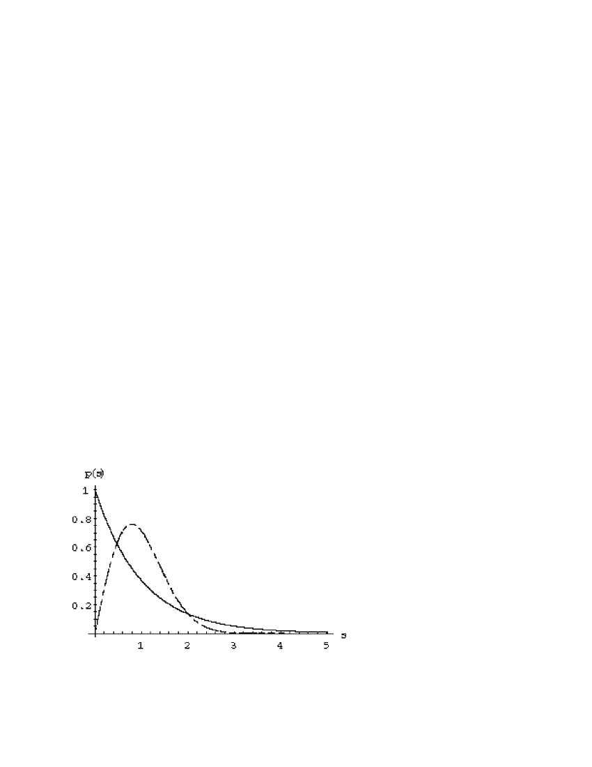
Figure 2: $P\left(s\right)_{W}$ Vs. $s$, $q=1.01$. The non-extensive and extensive Wigner distributions are nearly super-imposed. The Poisson distribution is plotted using a solid line.

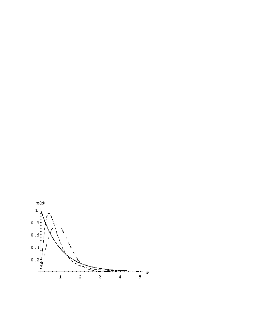
Figure 3: $P\left(s\right)_{W}$ Vs. $s$, $q=1.38$. The extensive distribution has been plotted with long-short dashing. The non-extensive Wigner distribution is plotted with the short dashes. The Poisson distribution is plotted using a solid line.

In this letter the Gaussian orthogonal ensemble (GOE) results for a $2\times 2$ random Hamiltonian matrix is generalized to the case of the non-extensive statistics and the resultant power-law distributions. A derivation of the subsequent level spacing statistical distribution, the non-extensive Wigner distribution, is given. This derivation is obtained by maximizing the Tsallis non-extensive entropy for the $2\times 2$ symmetrical random matrix elements. This can be straight-forwardly generalized to $M\times M$ matrices. The resultant non-extensive Wigner level-spacing distribution is $q$-parametrized and allows for a smooth interpolation between the extensive Wigner distribution and the regime where the level statistics are given by a Poisson distribution. In future work it will be interesting to apply these results to Hamiltonians of mixed systems between regular and chaotic regimes where deviations from the Wigner statistics become pronounced.

One of the authors, F. Michael, wishes to acknowledge support from the NSF through grant number DMR99-72683.

References

(1) T.A. Brody, J. Flores, J.B. French, P.A. Mello, A. Pandey, and S.S.M. Wong.
Random Matrix physics: spectrum and strength fluctuations. Rev. Mod. Phys. vol.53, pg.385 (1981).
(2) M.L. Mehta. Random Matrices. Academic press San Diego. 2nd edition (1991).
(3) F. Haake. Quantum Signatures of Chaos. 2nd edition. Springer (2000).
(4) H-J. Stockmann. Quantum Chaos, an Introduction. Cambridge Press (1999).
(5) C. Tsallis. J. Sta. Phys. vol.52, pg.479 (1988). C. Tsallis, R.S. Mendes,
A.R. Plastino, Physica A vol.261, pg.534 (1998). C. Tsallis, Braz. J. Phys. vol.29, pg.1 (1999).
(6) Q.A. Wang, Los Alamos preprint cond-mat/0009343.
(7) S. Abe and A.K. Rajagopal. quant-ph/0003145 (2000), and
references therein.