Edge overload breakdown in evolving networks

Abstract

We investigate growing networks based on Barabási and Albert’s algorithm for generating scale-free networks, but with edges sensitive to overload breakdown. The load is defined through edge betweenness centrality. We focus on the situation where the average number of connections per vertex is, as the number of vertices, linearly increasing in time. After an initial stage of growth, the network undergoes avalanching breakdowns to a fragmented state from which it never recovers. This breakdown is much less violent if the growth is by random rather than preferential attachment (as defines the Barabási and Albert model). We briefly discuss the case where the average number of connections per vertex is constant. In this case no breakdown avalanches occur. Implications to the growth of real-world communication networks are discussed.

I Introduction

Large sparse networks are the underlying structure for transportation or communication systems, both man made (like computer networks AJB ; otherCN or power grids PG ) or natural (like neural networks NN or biochemical networks BioC ). These networks displays both randomness and some self-induced structure influencing the flow of transport and robustness against congestion or breakdown in the network. One of the most conspicuous structures among real-world communication networks is a highly skewed distribution of the degree (the number of neighbors of a vertex) AJB ; otherCN ; otherSF .

Avalanching breakdown in networks where the edges or vertices are sensitive to overload is a serious threat for real-world networks. A recent example being the black-out of 11 US states and two Canadian provinces the 10th August 1996 blackout . Recently the overload breakdown problem for vertices in growing networks with an emerging power-law degree distribution has been studied EGO2 . In the present paper we investigate the overload breakdown problem when edges (rather than vertices) are sensitive to overloading. We use the standard model for such networks—the Barabási-Albert (BA) model BA1 ; BA2 , but with a maximum load capacity assigned to each edge. The load is defined by means of the betweenness centrality—a centrality measure for communication and transport flow in a network BC . The procedure enables us to study overload breakdown triggered by the redistribution (and increase) of load in a growing network. This is in contrast to earlier models of cascading breakdown phenomena, all dealing with vertex breakdown, that has taken a fixed network as their starting point WATTS ; MGP .

II Definitions

We represent networks as undirected and unweighted graphs $G=(V,E)$ where $V$ is the set of vertices, and $E$ is the set of unweighted edges (unordered pairs of vertices). Multiple edges between the same pair of vertices are not allowed.

II.1 The Barabási-Albert model of scale-free networks

The standard model for evolving networks with an emerging power-law degree distribution is the Barabási-Albert model. In this model, starting from $m_{0}$ vertices and no edges, one vertex with $m$ edges is attached iteratively. The crucial ingredient is a biased selection of what vertex to attach to, the so called “preferential attachment:” In the process of adding edges, the probability $P_{u}$ for a new vertex $v$ to be attached to $u$ is given by BA3

$$P_{u}=\frac{k_{u}+1}{\sum_{w\in V}(k_{w}+1)}~{},$$ (1)

where $k_{u}$ is the degree of the vertex $u$. To understand the effect of preferential attachment, we will also investigate networks grown with a unbiased random attachment of vertices. Without the preferential attachment the networks are known to have an exponential tail of the degree distribution BA2 . The time $t$ is measured as the total number of added edges, which is different by factor $m$ from Refs. BA1 ; BA2 where $t$ is defined as the number of added vertices.

It should be noted that in very large communication networks, such as the Internet, the users can process information about only a subset of the whole network. How this affects the dynamics of network formation is investigated in Ref. mossa . In the present work we neglect such effects and assume linear preferential attachment.

II.2 Load and capacity

To assess the load on the vertices of a communication network, or any network where contact between two vertices are established through a path in the network, a common choice is the betweenness centrality BC which often is seen as a vertex quantity but has a natural extension to edges $e\in E$ GN :

$$C_{B}(e)=\sum_{v\in V}\sum_{w\in V\setminus\{v\}}\frac{\sigma_{vw}(e)}{\sigma_{vw}}~{},$$ (2)

where $\sigma_{vw}(e)$ is the number of geodesics between $v$ and $w$ that contains $e$, and $\sigma_{vw}$ is the total number of geodesics between $v$ and $w$. $C_{B}(e)$ is thus the number of geodesics between pairs of vertices passing $e$; if more than one geodesics exists between $v$ and $w$ the fraction of vertices containing $e$ contributes to $e$’s betweenness.

In Ref. EGO2 (see also Ref. KAHNG ) the use of betweenness centrality as a load measure is given thorough motivations. These arguments are readily generalized to the case of edges sensitive to overloading: Suppose that $\Lambda$ is the set of pairs of vertices with established communications through shortest paths at a given instant foot . Then let $\lambda(e)$ denote the load of $e\in E$ defined as the number of geodesics that contains $e$. Then we assume the effective load to be the average

$$\langle\lambda(e)\rangle_{\Omega}=\frac{1}{|\Omega|}\sum_{\Lambda\in\Omega}\lambda(e),$$ (3)

where $\Omega$ is an ensemble of $\Lambda$. To proceed, we restrict $\Omega$ according to:

$$\Omega=\{\Lambda:|\Lambda|=AN(N-1)\},$$ (4)

where $A$ is constant with respect to $N$. This is to be interpreted that an element of $\Omega$ is a set of $AN(N-1)$ pairs of distinct vertices chosen uniformly at random, and thus corresponds to the case where the number of established communication routes ending at a specific vertex in average increases with $N$. This case can for example be expected in the early days of the Internet where the launches of new sites made the users browse a larger average number of sites. The case where the users at average connects to an $N$-independent number of others is discussed in Appendix A. The largest approximation, when using the betweenness as a load measure, is probably that routing protocols of e.g. the Internet has implicitly implemented load balancing foot ; OSPF ; huitema .

To introduce overloading to the dynamics we assign a capacity, or maximum value, $\lambda^{\mathrm{max}}(e)$ to the load, the same for each edge, and say that the edge $e$ is overloaded if $\lambda^{\mathrm{max}}(e)<\langle\lambda(e)\rangle_{\Omega}$. From the definition of $\Omega$ we can see that our situation corresponds to having a maximum capacity on the betweenness centrality of the edges so that an edge is overloaded if $C_{B}(e)>C_{B}^{\mathrm{max}}$ (where $C_{B}^{\mathrm{max}}$ is constant). If an edge is overloaded it is simply removed from the graph, and the betweenness recalculated, if then another edge becomes overloaded it is removed, and so on. If more than one edge is overloaded at a time we choose the one to remove randomly. Multiple breakdowns during one time step defines a “breakdown avalanche.”

II.3 Quantities for measuring network functionality

To measure the network functionality we consider three quantities—the number of edges $L$, inverse geodesic length $l^{-1}$, and the size of the largest connected subgraph $S$: For the original BA model the number of edges increases linearly as $L(t)=t$ (i.e. one edge is added in unit time). But if an overload breakdown occurs in the system $L$ decreases, making it a suitable simplest-possible-measure of the network functionality. In a functional network a large portion of the vertices should have the possibility to connect to each other. In percolation and attack vulnerability studies of random networks one often uses $S$ to define the system as ‘percolated’ (or functioning), when the size of the largest connected subgraph $S$ scales as $N$ AJB ; ATTPER . One of the characteristic features of the BA model networks, as well as many real-world communication networks, is a less than algebraically increasing average geodesic length $l$. As the average geodesic length is infinite when the network is disconnected (as could be the case when an overload breakdown has occurred) we study the average inverse geodesic length NEWMAN :

$$l^{-1}\equiv\left\langle\frac{1}{d(v,w)}\right\rangle\equiv\frac{1}{N(N-1)}\sum_{v\in V}\sum_{w\in V\setminus\{v\}}\frac{1}{d(v,w)}~{},$$ (5)

which has a finite value even for the disconnected graph if one defines $1/d(v,w)\equiv 0$ in the case that no path connects $v$ and $w$. To monitor the fragmentation of the network we will also measure the number of connected subgraphs $n$.

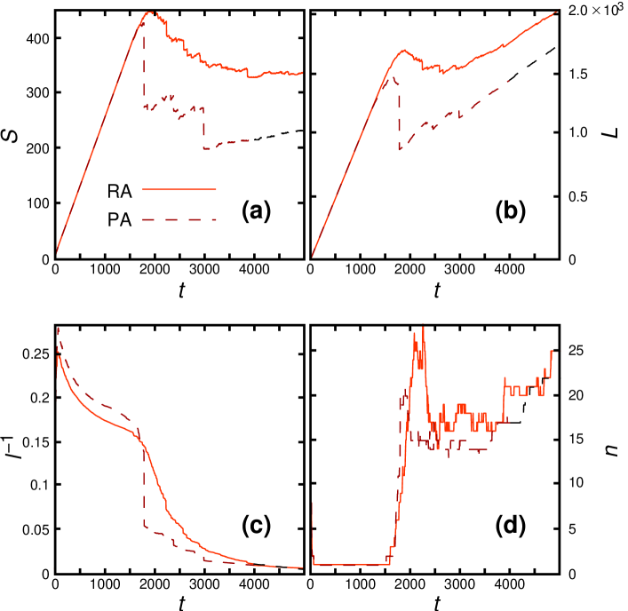
Figure 1: The time evolution of $S$ (a), $L$ (b), $l^{-1}$ (c), and $n$ (d) for a typical run with $C_{B}^{\mathrm{max}}=500$ and $m_{0}/2=m=4$. Dashed lines represent the network grown with preferential attachment (PA), solid grey lines denotes curves for the runs with an unbiased random attachment (RA).

III Simulation results

For relative small $m$, typical runs are exemplified in Fig. 1. For both random and preferential attachment $\langle S\rangle$ reaches a critical time where after the network starts to break down, eventually $\langle S\rangle$ reaches a steady state value. The breakdown develops differently in the two cases: For the random attachment the breakdown is relatively slow and the steady state value is high compared to the preferential attachment case where large successive avalanches fragments the network. The other two quantities reflects the same behavior: While the initial vertices gets joined into the network $l^{-1}$ increases to an early maximum. After the decrease corresponding to the increase of $l$, $l^{-1}$ decreases rapidly when the network becomes fragmented. $L$ shows the jagged shape, as expected correlated with that of $\langle S\rangle$. As seen in Fig. 1(a) and (b), the discontinuity in $L$ (in the preferential attachment case), is less pronounced than that in $\langle S\rangle$, so a small number of overloaded edges can be enough to cause large decrease in $\langle S\rangle$. The reason for this behavior is that bridges (single edges interconnecting connected subgraphs) have a high betweenness and thus are prone to overloading. The number of connected subgraphs behaves qualitatively the same for random and preferential attachment. For other runs of the algorithm the breakdown can qualitatively be described as above. The averaged quantities varies relatively little, for example the peak-time for $\langle S\rangle$ has a standard deviation of $\sim 3$%.

The corresponding overload case for vertices studied in Ref. EGO2 shows a similar time development with an period of incipient scale-freeness, an intermediate regime of breakdown and recovery (although the period of recovery is not as large for edges as for vertices), and a final breakdown to a large-$t$ state of disconnected clusters. One major difference between overload breakdown for vertices and edges is that the difference between random and preferential attachment is larger for edge overloading—edge robustness benefits more than vertex robustness from the geometry arising from random attachment.

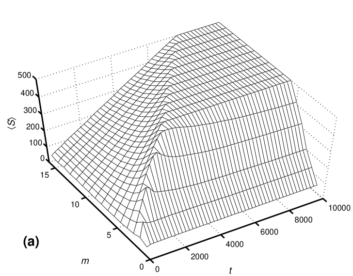
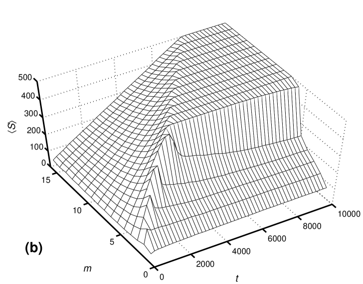
Figure 2: The $m$ dependence of the time development of $\langle S\rangle$—the average size of the largest connected subgraph with $C_{B}^{\mathrm{max}}=500$, and $m_{0}=2m$, for (a) random attachment and (b) preferential attachment.

Next we investigate the $m$-dependence. As seen in Fig. 2 the system becomes more and more robust when $m$ increases. This is of course expected since with a higher average degree more edges shares the load, so the maximal load can be expected to decrease. For high enough $m$ there are no avalanches, the largest connected component remains of the same size $S=C_{B}^{\mathrm{max}}+1$. When $S=C_{B}^{\mathrm{max}}+1$ the next edge attaching a new vertex will have $C_{B}(e)=C_{B}^{\mathrm{max}}+1$, and thus be overloaded. In most cases this will lead to removal of the newly added edge—otherwise another edge has to be overloaded at the same time, which is decreasingly likely with increasing $m$. In Fig. 2(b) we can see one exception to this interpretation at $m=6$: Here $\langle S\rangle$ reaches $C_{B}^{\mathrm{max}}+1$ but starts to decay slowly at around $t=8000$. As mentioned, the largest connected subgraph is expected to become more stable as $m$ increases. If there is an $m$ above which $\langle S\rangle=C_{B}^{\mathrm{max}}+1$ for arbitrary large $t$ above some $t_{0}$ is an open question. Comparing Fig. 2(a) and Fig. 2(b) shows that random attachment and preferential attachment have similar $m$-dependence behavior—the major difference being that preferential attachment has a much sharper increase of $\langle S\rangle$; to be more precise the $m$ values that does not reach $S=C_{B}^{\mathrm{max}}+1$ for any $t$, have a lower value in the large-$t$ limit.

Figure 3: Histograms (averaged over $10^{4}$ runs) of degree. The parameter values are $m=m_{0}/2=4$ and $C_{B}^{\mathrm{max}}=500$. (a) shows histograms for random attachment, (b) shows histograms for random attachment. The grey line in (b) is the function $38\,k_{v}^{-3}$ illustrating the emerging power-law degree distribution at early times.

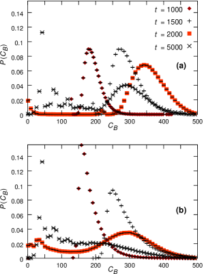
Figure 4: Histograms (averaged over $10^{4}$ runs) of edge betweenness centrality. The parameter values are—as in Fig, 3—$m=m_{0}/2=4$ and $C_{B}^{\mathrm{max}}=500$. (a) shows histograms for random attachment, (b) shows histograms for random attachment.

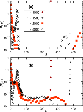
Figure 5: The distribution of sizes of connected clusters at different times for $m=m_{0}/2=4$, $C_{B}^{\mathrm{max}}=500$ and (a) random attachment, (b) preferential attachment. All curves represents averages over $10^{4}$ runs. To overcome noise the $t\geq 2000$ histograms are binned for $s\geq 75$, each point being an average over a width of 10.

To get another angle of the mechanisms of the breakdowns for small $m$, we consider histograms of degree $k_{v}$ and betweenness $C_{B}(e)$. Figs. 3 and 4 shows these histograms both before and after the large drop in $\langle S\rangle$ for $m=m_{0}/2=4$ and $C_{B}^{\mathrm{max}}=500$. (In the random attachment case this drop occurs at $t_{\mathrm{drop}}\approx 1600$, the corresponding value for preferential attachment is $t_{\mathrm{drop}}\approx 2000$.) For random attachment the difference between the histograms before and after the $\langle S\rangle$-drop is distinctively smaller than for preferential attachment, just as expected from Fig. 2. The random attachment curves in Fig. 3(a) has a degree distribution of truncated exponential form both at the earlier and later times. In Fig. 3(a) it is exponential over two decades of $P(k_{v})$, but falls off faster than exponentially for higher $k_{v}$. For preferential attachment the degree distributions (Fig. 3(b)) have a distinct difference—at $t<t_{\mathrm{drop}}$ there is an emergent power-law shape of the $P(k_{v})$-curve, whereas at $t>t_{\mathrm{drop}}$ the shape is exponential, $\sim\,\exp(-0.62\,k_{v})$, over five decades. To summarize, the degree distributions before and after the $\langle S\rangle$-peak illustrates the same behavior as the time evolution of $\langle S\rangle$—the breakdown in the preferential attachment case is both faster and more restructuring than in the random attachment case.

The betweenness distributions of Fig. 4 shows a peak that moves to higher $C_{B}$, as $t$ grows, until it reaches its maximal value at the time of the drop in $\langle S\rangle$ and starts to decrease. For random attachment (Fig. 4 (a)) the shape of the distribution looks qualitatively the same before and after the drop, but for preferential attachment (Fig. 4 (b)) $P(C_{B})\approx 0$ for betweenness smaller than the peak. The vertex betweenness distribution of the BA model is known to be strictly decreasing KAHNG , which would imply that the low-$C_{B}$ tails in Fig. 4 (b) (and most likely in Fig. 4 (a) as well) comes from a spread of the size of the largest cluster, rather than from a tail in the largest cluster’s betweenness distribution. Another feature of the betweenness histograms of Fig. 4 is the smaller peaks at low $C_{B}$ for $t<t_{\mathrm{drop}}$. These peaks corresponds to a sharp peak of the cluster size distribution just after the $\langle S\rangle$-peak (see Fig. 5). Such smaller clusters have small average degree with many $k_{v}=1$ vertices, which all contributes to a peak at $s$ of the betweenness histograms. This explains the peak at $C_{B}\approx 45$ in the $t=5000$ curve of Fig. 4 (b).

The distribution of cluster sizes displayed in Fig. 5 gives some further insights: For $t>t_{\mathrm{drop}}$ of the random attachment curves shows a bimodal distribution as $P(s)$ is zero in the interval $60\lesssim s\lesssim 290$. The preferential attachment curves, in contrast, has a long tail. Both the large $s$ peak for random attachment and the tail of preferential attachment corresponds to one single cluster. This is in striking contrast to the vertex overload case EGO2 where the network looses the unique largest component after the breakdown avalanches. As $t$ evolves well beyond $t_{\mathrm{drop}}$ the largest component peak decreases, and does thus not represent a giant component (a largest cluster proportional to $N$). The picture for both random and preferential attachment is thus that the system does not loose its unique largest cluster in a single breakdown avalanche—an avalanche rather results in a few isolated vertices or smaller clusters getting disconnected from the largest connected component.

The overall picture of the time evolution of $\langle S\rangle$, $L$ and $l^{-1}$ (Fig. 1), the $m$-dependence (Fig. 2), as well as the histograms of Figs. 3, 4 and 5 is that for small $m$, avalanching breakdowns fragments the network to a state from which it never recovers. For preferential attachment the newly fragmented network contains a single largest cluster with a well defined size, and the emergent scale-free degree distribution before $t_{\mathrm{drop}}$ is replaced by an exponential distribution. The breakdown for the random attachment case turns out to be less violent, and does not cause any major structural change. Furthermore, the difference between the random and preferential attachment cases is larger for edge breakdown than for the corresponding vertex breakdown model studied in Ref. EGO2 .

IV Summary and conclusions

We have studied networks grown by the Barabási-Albert model for networks with emergent scale-freeness and edges sensitive to overloading. Except the preferential attachment defining the BA model, we also study an unbiased random attachment. We focus on the case where the number of established connections to random other vertices of the network scales linearly with the number of vertices in the network.

We find that for intermediate values of $m$ (the number of edges added per vertex) the network grows like the BA model up to a point where is starts to break down. After a number of avalanching breakdowns the network reaches a state characterized by many disconnected clusters from which a giant component never re-emerges (although, in the preferential attachment case, there will always be one single largest cluster much larger than any other). If the growth is by random attachment, the breakdown is less violent with smaller avalanches and no pronounced structural change. For large $m$ the steady state at large times is characterized by a constant largest cluster size.

In context of real world communication networks one can conclude that these would benefit from being grown by random rather than preferential attachment (and this difference being larger for edge overload than for vertex overload studied in Ref. EGO2 ). In the vertex overload case avalanches proceeds until the network is fragmented into small clusters; in the edge overload problem there is still one large component after the breakdowns, thus we infer that for real-world communication networks, vertex overloading is a greater threat than edge overloading, and congestion control in telecommunication networks kihl and Internet routing protocols huitema should focus on balancing the vertex rather than edge load. Only if the capacity of vertices (servers etc.) grows significantly faster than the capacity for edges (cables etc.), edge overload breakdown is a potential threat for avalanching breakdowns that is triggered by the change of load in a growing network.

Appendix A Intrinsic communication activity

This paper deals mainly with the case where the average user of a growing communication network communicates with a number of others that increases linearly with $N$. One can also imagine a case where, even though the network grows, the users in average communicates with a network size independent number of others; which is the topic of the present Appendix. (In Ref. EGO2 this scenario was termed “intrinsic communication activity.”) The behavior of real communication networks lies, presumably, between these two extremes.

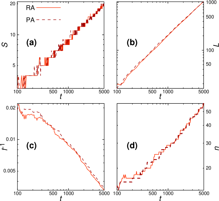
Figure 6: The time evolution of $S$ (a), $L$ (b), $l^{-1}$ (c), and $n$ (d) for a typical run in the intrinsic communication activity case. The model parameters are: $c_{B}^{\mathrm{max}}=0.1$ and $m_{0}/2=m=5$. Dashed lines represent the network grown with preferential attachment (PA), solid grey lines denotes curves for the runs with an unbiased random attachment (RA).

A.1 Definitions

To implement the situation of intrinsic communication activity, we modify Eq. 4 to:

$$\Omega^{\prime}=\{\Lambda:|\Lambda|=A^{\prime}N\}$$ (6)

where $A^{\prime}$ is constant with respect to $N$. I.e. the users has the $N$-independent average number $A^{\prime}$ of established contacts through shortest routes. Averaging the load over $\Omega^{\prime}$ according to Eq. 3 gives:

$$\langle\lambda(e)\rangle_{\Omega^{\prime}} = \frac{1}{|\Omega^{\prime}|}\sum_{\Lambda\in\Omega^{\prime}}\sum_{(w,w^{\prime})\in\Lambda}\frac{\sigma_{w\,w^{\prime}}(e)}{\sigma_{w\,w^{\prime}}}$$ (7)

$$= \frac{A^{\prime}}{N}\,C_{B}(e)~{}.$$

From this we see that having a constant capacity for the load $\lambda(e)$ corresponds to having a limit on $C_{B}(e)$ that increases with $N$. Thus we view $e$ as overloaded if $C_{B}(e)$ exceeds $C_{B}^{\mathrm{max}}=Nc_{B}^{\mathrm{max}}$ (where $c_{B}^{\mathrm{max}}$ is constant).

A.2 Results

In the vertex overload breakdown problem, the case of intrinsic communication activity has a more complex dynamics than the extrinsic communication activity case (studied in the main part of the text), with giant components forming only occasionally for some sets of parameter values EGO2 . For edge overload breakdown, on the other hand, the dynamics of a system with intrinsic communication activity seems very simple with no avalanching breakdowns and no qualitative difference between preferential and random attachment, see Fig. 6. We can also notice that the measured quantities has a power-law dependence of $t$. (Fig. 6 is constructed from one run with random and preferential attachment respectively.) For large times ($1000\lesssim t\lesssim 5000$) the exponent $\alpha$ for the time development of the respective quantity is (in the large $t$ limit): $\alpha_{l^{-1}}\approx-0.6$, $\alpha_{L}=1.0$, and $\alpha_{S}=\alpha_{n}=0.50$ for both (a) and (b). Initially $\alpha_{l^{-1}}$ is closer to zero, for $100\lesssim t\lesssim 1000$ we have $\alpha_{l^{-1}}\approx-0.5$. To illustrate the consistency of the exponents we note that

$$\sum_{e\in E}C_{B}(e)=\sum_{v\in V}\sum_{w\in V\setminus\{v\}}d(v,w)=n\frac{N}{n}\left(\frac{N}{n}-1\right)\langle l_{\mathrm{CS}}\rangle~{},$$ (8)

where $\langle l_{\mathrm{CS}}\rangle$ is the average geodesic length for a connected subgraph, and $d(v,w)=0$ if $v$ and $w$ are disconnected. This yields

$$\langle C_{B}(e)\rangle\approx m\left(\frac{N}{n}-1\right)l_{\mathrm{CS}}\leq\max_{v\in V}C_{B}(e)~{}.$$ (9)

If one assumes that $\langle C_{B}(e)\rangle\propto\max_{v\in V}C_{B}(e)$ and $N\gg n$ we have $\langle l_{\mathrm{CS}}\rangle\propto n$. Making the crude approximation $l^{-1}\approx\langle l_{\mathrm{CS}}\rangle^{-1}$ gives $\alpha_{l^{-1}}\approx-\alpha_{n}$, which holds well for small $t$. As $t$ increases the spread in shape of the connected subgraphs becomes larger so the $l^{-1}\approx\langle l_{\mathrm{CS}}\rangle^{-1}$ approximation becomes worse which is seen as a slight increase of the slope $\alpha_{l^{-1}}$. That the approximation $\alpha_{l^{-1}}\approx-\alpha_{n}$ is rather good throughout the range of $t$ is also reflected in that the average size of connected components $N/n$ is never very far from $S$: At $t=5000$ we have (see Fig. 6(a)) $N/n\approx 50$ and $S=57$ for random attachment, and $N/n\approx 53$ and $S=56$ for preferential attachment. In this approximation we see that $l\propto n\propto N^{1/2}$ so the small average geodesic length is lost within the connected subgraphs. If $c_{B}^{\mathrm{max}}$ is chosen larger, so the network initially grows without edges breaking, there are no large avalanches but a crossover to the behavior seen in Fig. 6.

References

- (1) R. Albert, H. Jeong, and A.-L. Barabási, Nature (London) 401, 130 (1999).
- (2) M. Faloutsos, P. Faloutsos, and C. Faloutsos, Comput. Commun. Rev. 29, 251 (1999); R. Kumar, P. Rajalopagan, C. Divakumar, A. Tomkins, and E. Upfal, in Proceedings of the 19th Symposium on Principles of Database Systems (Association for Computing Machinery, New York, 1999); A. Broder et al., Comput. Netw. 33, 309 (2000); R. Pastor-Santorras, R. A. Vázquez, and A. Vespignani, Phys. Rev. Lett. 87, 258791 (2001).
- (3) D. J. Watts and S. H. Strogatz, Nature (London) 393, 440 (1998); D. J. Watts, Small Worlds (Princeton University Press, Princeton NJ, 1999).
- (4) L. A. N. Amaral, A. Scala, M. Barthélémy, and H. E. Stanley, Proc. Nat. Acad. Sci. USA 97, 11149 (2000); O. Sporns, G. Todoni, and G. M. Edelman, Cerebral Cortex 10, 127 (2000).
- (5) H. Jeong, B. Tombor, R. Albert, Z. N. Oltvai, and A.-L. Barabási, Nature (London) 407, 651 (2000); D. A. Fell and A. Wagner, Nature Biotechnol. 18, 1121 (2000); H. Jeong, S. P. Mason, A.-L. Barabási, and Z. N. Oltvai, Nature (London) 411, 42 (2001).
- (6) M. E. J. Newman, Phys. Rev. E 64, 016131 (2001); 016132 (2001); F. Liljeros, C. R. Edling, L. A. N. Amaral, H. E. Stanley, and Y. Åberg, Nature (London) 411, 907 (2001).
- (7) See e.g. S. H. Strogatz, Nature (London) 410, 268 (2001).
- (8) P. Holme and B. J. Kim, Phys. Rev. E 65, 066109 (2002).
- (9) A.-L. Barabási and R. Albert, Science 286, 509 (1999).
- (10) A.-L. Barabási, R. Albert, and H. Jeong, Physica A 272, 173 (1999).
- (11) J. M. Anthonisse, Stichting Mathematisch Centrum, Technical Report BN 9/71, 1971 (unpublished); M. L. Freeman, Sociometry 40, 35 (1977).
- (12) D. J. Watts, Proc. Nat. Acad. Sci. USA 99, 5766 (2002).
- (13) Y. Moreno, J. B. Gómez, and A. F. Pacheco, Europhys. Lett. 58, 630 (2002).
- (14) R. Albert and A.-L. Barabási, Phys. Rev. Lett. 85, 5234 (2000).
- (15) S. Mossa, M. Barthélémy, H. E. Stanley, and L. A. N. Amaral, Phys. Rev. Lett. 88, 138701 (2002).
- (16) M. Girvan and M. E. J. Newman, Proc. Nat. Acad. Sci. USA 99, 7821 (2002).
- (17) K.-I. Goh, B. Kahng, and D. Kim, Phys. Rev. Lett. 87, 278201 (2001).
- (18) A centrality measure reflecting the flow in a system with load balancing is the “flow betweenness:” L. C. Freeman, S. P. Borgatti, and D. R. White, Social Networks 13, 141 (1991). The outcome of the present study with betweenness replaced by flow betweenness is an interesting open question.
- (19) Nevertheless, choosing the shortest routes is the first principle of some real Internet routing protocols such as the Open Shortest Path First (OSPF) protocol. J. T. Moy, OSPF: Anatomy of an Internet Routing Protocol (Addison-Wesley, Reading MA, 1998).
- (20) C. Huitema, Routing in the Internet 2nd ed. (Prentice Hall, Upper Saddle River NJ, 2000).
- (21) To calculate the betweenness centrality we use the algorithm presented in U. Brandes, J. Math. Sociol. 25, 163 (2001). An equally efficient algorithm was proposed in M. E. J. Newman, Phys. Rev. E 64, 016132 (2001).
- (22) M. E. J. Newman and D. J. Watts, Phys. Lett. A 263 341 (1999); M. E. J. Newman and D. J. Watts, Phys. Rev. E 60, 7332 (1999); C. Moore and M. E. J. Newman, ibid. 61, 5678 (2000); C. Moore and M. E. J. Newman, ibid. 62, 7059 (2000); R. Albert, H. Jeong, and A.-L. Barabási, Nature (London) 406, 378 (2000); M. Ozana, Europhys. Lett. 55, 762 (2001); P. Holme, B. J. Kim, C. N. Yoon, and S. K. Han, Phys. Rev. E 65, 056109 (2002).
- (23) M. E. J. Newman, J. Stat. Phys. 101, 819 (2000).
- (24) In the Erdős-Rényi (ER) model edges are attached to vertices with no multiple edges being the only constraint. These networks have a exponential tail of the degree distribution. For the ER model, see P. Erdős and A. Rényi, Publ. Math. Inst. Hung. Acad. Sci. 5, 17 (1960).
- (25) M. Kihl, Overload Control Strategies for Distributed Communication Networks (Lund University Press, Lund, 1999).