Parametric Statistics of Individual Energy Levels in Random Hamiltonians

Abstract

We establish a general framework to explore parametric statistics of individual energy levels in disordered and chaotic quantum systems of unitary symmetry. The method is applied to the calculation of the universal intra-level parametric velocity correlation function and the distribution of level shifts under the influence of an arbitrary external perturbation.

Ensembles of random Hamiltonians are used frequently to model properties of diverse physical systems. Although eigenfunction statistics can play an important role in some applications, typically one is interested in the statistics of the spectra $\{\epsilon_{i}\}$ of such Hamiltonians. Among all the possible statistical ensembles Zirnbauer a special role is played by the three invariant Dyson distributions mehta . Characterized by the assumption that the distribution is invariant under, respectively, orthogonal, unitary, and symplectic rotations of the basis, the random matrix theory (RMT) has proved to be remarkably successful in modeling physical systems ranging from nuclear spectra porter and mesoscopic quantum dots reviews to individual chaotic quantum structures BGS .

An important class of problems arise when individual members $H$ of the statistical ensemble undergo parametric evolution according to the rule $H\rightarrow H^{\prime}=H+XV$, where $V$ is a fixed matrix, and $X$ is the strength of the perturbation. Instead of the random variables $\epsilon_{i}$, one is now confronted with random functions $\epsilon_{i}(X)$ of the external parameter $X$. Once cast in terms of the rescaled variable $x=X\sqrt{\langle(\partial_{X}\epsilon_{i})^{2}\rangle}$ (all energies being measured in the units of the mean level spacing $\Delta$), it has been argued SA that, for a generic perturbation $V$ (see below), the statistical properties of the entire random functions $\epsilon_{i}(x)$ exhibit the same degree of universality as that of the parent Hamiltonian $H$. As well as mesoscopic and chaotic quantum structures, universality of the random functions $\epsilon_{i}(x)$ finds application to a variety of physical systems including step configurations on vicinal surfaces teinstein , non-intersecting random walkers in one dimension forrester , and the world lines of one-dimensional fermions SA .

Beginning with the seminal work of Dyson Dyson , the statistical properties of the random functions $\{\epsilon_{i}(x)\}$ have been the subject of numerous investigations list (for a review, see, e.g., Ref. efetov ). To date, exact analytic expressions have been obtained for the distribution of “local” (in the parameter space) properties such as “level velocities” $\partial_{x}\epsilon_{i}(x)$ SA ; eduardo1 ; MSS and “level curvatures” $\partial_{x}^{2}\epsilon_{i}(x)$ vonOppen . At the same time, parametric correlations between the sets $\{\epsilon_{i}(\bar{x})\}$ and $\{\epsilon_{i}(\bar{x}+x)\}$ have been explored SA using field theoretic techniques efetov . As well as establishing the range of universality, explicit expressions for the parametric correlator of the density of states (DoS) and the related level velocity correlation function $\tilde{c}(\omega,x)=\langle\sum_{ij}\partial_{\bar{x}}\epsilon_{i}(\bar{x})\partial_{\bar{x}}\epsilon_{j}(\bar{x}+x)\delta(\epsilon-\epsilon_{i}(\bar{x}))\delta(\epsilon+\omega-\epsilon_{j}(\bar{x}+x))\rangle$ have been inferred.

When RMT is applied to many-fermion systems, an important distinction arises between two classes of correlation functions: Employing the terminology somewhat loosely, the function $\tilde{c}(\omega,x)$ can be termed “grand canonical” in the sense that the level $\epsilon_{j}(\bar{x}+x)$ need not be a parametric “descendant” of the level $\epsilon_{i}(\bar{x})$. Indeed, the definition of $\tilde{c}(\omega,x)$ tracks correlations between $\epsilon_{i}(\bar{x})$ and a “descendant” of any other level. However, often one is interested in the parametric evolution of the Fermi level or a low-lying excitation in systems with a fixed number of fermions. Inasmuch as such a level can be interpreted as a single particle level of some effective random many-body Hamiltonian, the relevant objects are the “canonical” correlation functions, exemplified by the intra-level velocity correlation function

$$c(x)\equiv\left\langle\partial_{\bar{x}}\epsilon_{i}(\bar{x})\partial_{\bar{x}}\epsilon_{i}(\bar{x}+x)\right\rangle.$$ (1)

A different perspective is provided by the distribution of single-level shifts

$$p(\omega,x)\equiv\left\langle\delta\left(\epsilon_{i}\left(\bar{x}+x\right)-\epsilon_{i}\left(\bar{x}\right)-\omega\right)\right\rangle.$$ (2)

Apart from their intrinsic interest, it has been argued reviews that the functions $c(x)$ and $p(\omega,x)$ describe parametric correlations of resonant conductance peaks of quantum dots driven into the Coulomb Blockade regime and perturbed by a magnetic field or an external gate potential. Similarly, once $x$ is identified with magnetic flux, $c(x)$ coincides with the ensemble-averaged correlation function of single-level persistent currents efetov .

To date, studies of parametric correlations of individual energy levels have been limited to numerical investigations. Despite its affinity with $\tilde{c}(\omega,x)$, the intra-level correlation function $c(x)$ (and its canonical counterparts) belong to a different class of objects. Its analysis presents technical difficulties which are, in part, similar to the challenges encountered in the calculation of the level spacing distribution in non-parametric random matrix ensembles. The latter are known to engage DoS correlations which go beyond the two-point averages presently accessible by field theoretic techniques, and lead to expressions in terms of Fredholm determinants with integrable kernels mehta .

The aim of the present letter is to formulate a general framework to explore parametric correlations of individual energy levels. In particular, for the unitary random matrix ensemble, we will show that

$$c(x)=\int_{-\infty}^{\infty}d\omega\int_{0}^{2\pi}\frac{d\phi}{2\pi}\frac{1}{z_{+}z_{-}}\left(-\partial_{x}^{2}\right)Z(\omega,x;\phi)\qquad$$ (3)

$$p(\omega,x)=\int_{0}^{2\pi}\frac{d\phi}{2\pi}\frac{1}{z_{+}z_{-}}\left(-\partial_{\omega}^{2}\right)Z(\omega,x;\phi)$$ (4)

where $z_{\pm}(\phi)=1+e^{\pm i\phi}$ and, adopting the shorthand notation $\openone$ to represent the Dirac $\delta$-function,

$$Z\left(\omega,x;\phi\right)=\det_{\left[-1,1\right]}\left(\openone-\hat{\mathcal{K}}\left(\phi\right)\right).$$ (5)

The operator kernel $\hat{\mathcal{K}}\left(\phi\right)$ has matrix elements

$${\mathcal{K}}\left(\lambda,\mu;\phi\right)=\frac{1}{4\pi i}\sqrt{{\mathcal{D}}\left(\lambda\right){\mathcal{D}}\left(\mu\right)}\frac{F(\lambda;\phi)-F(\mu;\phi)}{\lambda-\mu},$$ (6a)

where

$$F(\lambda;\phi)=\frac{(z_{+}+z_{-})}{\pi i}\,\mathchoice{{\vbox{\hbox{$\textstyle-$}}\kern-4.86108pt}}{{\vbox{\hbox{$\scriptstyle-$}}\kern-3.25pt}}{{\vbox{\hbox{$\scriptscriptstyle-$}}\kern-2.29166pt}}{{\vbox{\hbox{$\scriptscriptstyle-$}}\kern-1.875pt}}\!\int_{-\infty}^{\infty}\!\!d\mu\frac{{\mathcal{D}}^{-1}(\mu)}{\mu-\lambda}-(z_{+}-z_{-})\,{\mathcal{D}}^{-1}(\lambda)$$ (6b)

Here the integral is understood in the sense of the Cauchy principal value, with variables $\lambda$ and $\mu$ restricted to the interval $\left[-1,1\right]$, and the dependence on $x$ and $\omega$ is encoded in the function

$${\mathcal{D}}\left(\lambda\right)=\exp\left[i\pi\omega\lambda+\pi^{2}x^{2}\lambda^{2}/2\right].$$ (7)

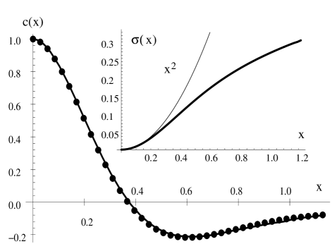
Figure 1: Level velocity correlation function obtained from Eqs. (3), (5-7) (solid line) vs. direct numerical simulation of large random matrices eduardo (dots). The width $\sigma\left(x\right)$ of the Gaussian distribution of level shifts together with the $x^{2}$ asymptotics at small $x$ is shown in the inset.

It is interesting to note that, after the substitution $x^{2}\mapsto-it$, at $\phi=0$, the integral kernel $\hat{\mathcal{K}}$ coincides with that arising in the calculation of time-dependent correlation functions of the one-dimensional interacting Bose gas at zero temperature Izergin . A comparison of the universal function $c(x)$ as inferred from Eqs. (3), (5-7) with the results of direct numerical simulation is shown in Fig. 1.

Before outlining the derivation of these results, several remarks are in order: (i) The universality of Eqs. (6) can be inferred from the universality of Eq. (13) below SA . As such, these results can be applied to the parametric evolution of spectra which obey Dyson statistics only “locally”. (ii) Although we have not succeeded in obtaining a direct proof, in accordance with the conjecture made in Ref. vallejos , the distribution of single-level shifts appears to assume a Gaussian form $p\left(\omega,x\right)=e^{-\omega^{2}/2\sigma(x)}/\sqrt{2\pi\sigma(x)}$ at any value of $x$. The corresponding width of the Gaussian can be expressed as

$$\sigma(x)\equiv\left\langle\left[\epsilon_{i}(\bar{x}+x)-\epsilon_{i}(\bar{x})\right]^{2}\right\rangle=2\int_{0}^{x}dx^{\prime}(x-x^{\prime})c(x^{\prime}).$$

At small $x$, where $p(\omega,x)$ can be inferred from the level velocity distribution SA ; eduardo1 , $\sigma\left(x\right)\stackrel{{\scriptstyle x\to 0}}{{=}}x^{2}$, which reflects (identifying time with $x^{2}$) independent “diffusion” of individual levels. In the opposite limit $x\mapsto\infty$, making use of the known asymptotic dependence SA $c(x)\stackrel{{\scriptstyle x\to\infty}}{{=}}-1/\pi^{2}x^{2}$ obtained from a perturbative analysis, one can infer the limiting behavior $\sigma(x)\stackrel{{\scriptstyle x\to\infty}}{{=}}\mathrm{const.}+(2/\pi^{2})\ln x$. The resulting strongly sub-diffusive behavior at large $x$ can be ascribed to the rigidity of the spectrum “hemming in” the meandering levels. (iii) The generating function $Z$ is a particular case of a more general object $\tilde{Z}_{q}(J,J^{\prime};x;\phi)$ which defines

$$P_{q}(J,J^{\prime};x)=\int_{0}^{2\pi}\frac{d\phi}{2\pi}e^{iq\phi}\tilde{Z}_{q}(J,J^{\prime};x;\phi)$$ (8)

as the probability that the number $n(J)$ of levels $\{\epsilon_{i}(\bar{x})\}$ in the (not necessarily contiguous) interval $J$ and the number $n^{\prime}(J^{\prime})$ of levels $\{\epsilon_{i}(\bar{x}+x)\}$ in the interval $J^{\prime}$ differ by exactly $q$. Taking $J$ and $J^{\prime}$ to be semi-infinite intervals $J_{\epsilon}=\left(-\infty,\epsilon\right]$ and $J_{\epsilon+\omega}=\left(-\infty,\epsilon+\omega\right]$, one can derive generalizations of Eqs. (3) and (4) which involve correlations between levels $\epsilon_{i}(\bar{x})$ and $\epsilon_{i+q}(\bar{x}+x)$:

$$c_{q}(x)\equiv\left\langle\partial_{\bar{x}}\epsilon_{i}(\bar{x})\partial_{\bar{x}}\epsilon_{i+q}(\bar{x}+x)\right\rangle$$ (9)

$$=(-1)^{q}\int_{-\infty}^{\infty}\!\!\!d\omega\int_{0}^{2\pi}\!\!\frac{d\phi}{2\pi}\frac{e^{iq\phi}}{z_{+}z_{-}}\left(-\partial_{x}^{2}\right)\tilde{Z}_{q}(J_{\epsilon},J_{\epsilon+\omega};x;\phi),$$

$$p_{q}(\omega,x)\equiv\left\langle\delta\left[\epsilon_{i+q}(\bar{x}+x)-\epsilon_{i}(\bar{x})-\omega\right]\right\rangle$$ (10)

$$=(-1)^{q}\int_{0}^{2\pi}\frac{d\phi}{2\pi}\frac{e^{iq\phi}}{z_{+}z_{-}}\left(-\partial_{\omega}^{2}\right)\tilde{Z}_{q}(J_{\epsilon},J_{\epsilon+\omega};x;\phi).$$

The exact analytic expression for $\tilde{Z}$ will be given below. (iv) In some applications, the fixed perturbation $XV$ may be of finite rank; i.e., it may possess only a finite number $r$ of non-zero eigenvalues SMS . In such situations Eqs. (6) retain their validity providing ${\mathcal{D}}(\lambda)$ is replaced by $e^{i\pi\omega\lambda}\det_{\mathrm{s}c}(1-i\lambda{\mathcal{R}})$, where ${\mathcal{R}}$ is the reactance matrix for scattering off the potential $XV$ MSS , and $\det_{\mathrm{s}c}$ denotes the determinant in the space of scattering channels. In this case $x$ may be identified with any of the variables parametrizing ${\mathcal{R}}$. (v) Despite the existence of well-developed analytical tools for the study of integral kernels with the structure of (6a) Izergin , it is at present unclear whether these methods can be generalized to accommodate $\phi$ integration in Eqs. (3) and (4).

The analysis of parametric statistics of individual energy levels relies on a technical device which ensures that the level $\epsilon_{i}(\bar{x}+x)$ is indeed the “descendant” of $\epsilon_{i}(\bar{x})$ by demanding that it has the same ordinal number as counted from the bottom of the spectrum. Specifically, due to the absence of level crossings, the intra-level velocity correlation function coincides with the conditional average

$$c(x)=\int_{-\infty}^{\infty}d\omega\langle\delta_{n(J_{\epsilon}),n^{\prime}(J_{\epsilon+\omega})}$$

$$\times\sum_{ij}\partial_{\bar{x}}\theta\left[\epsilon-\epsilon_{i}(\bar{x})\right]\partial_{\bar{x}}\theta\left[\epsilon+\omega-\epsilon_{j}(\bar{x}+x)\right]\rangle,\qquad$$ (11)

where $\delta_{n,n^{\prime}}$ denotes the Kronecker $\delta$-symbol, and $\theta$ is the step-function. The corresponding distribution of level shifts $p(\omega,x)$ is given by an analogous expression with $\partial_{\bar{x}}$ replaced by $\partial_{\epsilon}$ (and no integration over $\omega$). By generalizing the corresponding non-parametric formula for $P_{n}(J)$ footnote , our starting point is the general expression for the probability $P_{nn^{\prime}}(J,J^{\prime})$ to find $n$ levels in the interval $J$ of the unperturbed sequence and $n^{\prime}$ levels in the interval $J^{\prime}$ of the perturbed sequence,

$$P_{nn^{\prime}}(J,J^{\prime})=\frac{\left(-1\right)^{n+n^{\prime}}}{n!n^{\prime}!}\sum_{k=n}^{\infty}\sum_{k^{\prime}=n^{\prime}}^{\infty}\frac{\left(-1\right)^{k+k^{\prime}}r_{kk^{\prime}}}{\left(k-n\right)!\left(k^{\prime}-n^{\prime}\right)!}.$$ (12)

Here $r_{kk^{\prime}}$ represents the multi-point parametric correlation function of DoS SA ; SMS integrated over the interval $J^{k}\otimes J^{\prime k^{\prime}}$ with the corresponding measures $d\mu_{J}$ and $d\mu_{J^{\prime}}$. Owing to the determinantal structure of the DoS correlation function, $r_{kk^{\prime}}$ can be represented in the form of a fermionic functional integral

$$r_{kk^{\prime}}=\det K\int{\mathcal{D}}\Psi{\mathcal{D}}\bar{\Psi}\left(\int d\mu_{J}(u)\bar{\xi}(u)\xi(u)\right)^{k}\left(\int d\mu_{J^{\prime}}(w)\bar{\eta}(w)\eta(w)\right)^{k^{\prime}}e^{\int du\int dw\bar{\Psi}\left(u\right)K^{-1}\left(u,w\right)\Psi\left(w\right)}$$ (13)

where $\bar{\Psi}=\left(\bar{\xi},\bar{\eta}\right)$ is a fermionic doublet. Here

$$\hat{K}=\left(\begin{array}[]{cc}\hat{k}&\hat{\mathcal{D}}_{0}^{-1}\left[\hat{k}-\openone\right]\\ \hat{\mathcal{D}}_{0}\hat{k}&\hat{k}\end{array}\right),$$ (14)

where the matrix elements of the operator sine kernel $\hat{k}$ of the unitary Dyson ensemble are $k(u-w)=\sin\pi(u-w)/\pi(u-w)$, and $[\hat{\mathcal{D}}_{0}\hat{k}](u,w)=e^{-(x^{2}/2)d^{2}/du^{2}}k(u-w)$. Fixing the difference $n^{\prime}-n=q$ and summing over all $n$, one obtains the probability $P_{q}(J,J^{\prime};x)$ that the numbers of levels in the two intervals $J$ and $J^{\prime}$ differ by $q$:

$$P_{q}(J,J^{\prime};x)=\sum_{n=0}^{\infty}\frac{1}{n!(n+q)!}\!\!\sum_{\begin{subarray}{c}k=n\\ k^{\prime}=n+q\end{subarray}}^{\infty}\frac{\left(-1\right)^{k+k^{\prime}+q}r_{kk^{\prime}}}{\left(k-n\right)!\left(k^{\prime}-n-q\right)!}$$

$$=\int_{0}^{2\pi}\!\!\!\frac{d\phi}{2\pi}e^{iq\phi}\sum_{\begin{subarray}{c}k=0\\ k^{\prime}=q\end{subarray}}^{\infty}\frac{\left(-1\right)^{k+k^{\prime}+q}r_{kk^{\prime}}}{k!k^{\prime}!}z_{+}^{k}z_{-}^{k^{\prime}}$$ (15)

Substituting Eq. (13) into Eq. (Parametric Statistics of Individual Energy Levels in Random Hamiltonians), one finds

$$P_{q}\left(J,J^{\prime};x\right)=(-1)^{q}\int_{0}^{2\pi}\frac{d\phi}{2\pi}e^{iq\phi}\Bigg{\{}\det\left[\openone\sigma_{0}-\hat{K}\Pi\left(\phi\right)\right]$$

$$-\left.\left.\sum_{k^{\prime}=0}^{q-1}\frac{\partial_{\gamma}^{k^{\prime}}}{k^{\prime}!}\det\left[\openone\sigma_{0}-\hat{K}\Pi_{\gamma}\left(\phi\right)\right]\right|_{\gamma=0}\right\},$$ (16)

where

$$\Pi\left(\phi\right)=\left(\begin{array}[]{cc}z_{+}&0\\ 0&z_{-}\end{array}\right),\,\,\,\Pi_{\gamma}\left(\phi\right)=\left(\begin{array}[]{cc}z_{+}&0\\ 0&\gamma z_{-}\end{array}\right),$$

and $\sigma_{i}$ are the Pauli matrices. The determinants are understood as functional determinants on the space of two-component functions defined on the product interval $J\otimes J^{\prime}$. The expression in curly brackets in Eq. (Parametric Statistics of Individual Energy Levels in Random Hamiltonians) can be identified as the generating function $\tilde{Z}$.

In order to apply Eq. (Parametric Statistics of Individual Energy Levels in Random Hamiltonians) to the computation of the intra-level velocity correlation function and the distribution of the parametric level shifts, one must set $J=J_{\epsilon}$ and $J^{\prime}=J_{\epsilon+\omega}$. Setting $q=0$ and using Eq. (Parametric Statistics of Individual Energy Levels in Random Hamiltonians), one obtains Eqs. (3) and (4), where $Z$ is identified with the first determinant in Eq. (Parametric Statistics of Individual Energy Levels in Random Hamiltonians). For $q\neq 0$, a similar procedure leads to Eqs. (9) and (10).

The use of semi-infinite intervals to define $n(J_{\epsilon})$ and $n^{\prime}(J_{\epsilon+\omega})$ is justified only if the support of the spectrum is finite. The latter condition would be trivially fulfilled if one were to use, instead of $k(u-w)$, the exact Christoffel-Darboux kernel of the GUE whose scaling limits interpolate between the sine kernel inside the Wigner semicircle, and the Airy kernel at its endpoints. However, in practice, employing such a kernel would present significant technical difficulties. To circumvent this problem, we use a regularized kernel

$$k_{\delta}\left(u-w\right)=\frac{\sin\pi\left(u-w\right)}{\pi\left(u-w\right)}e^{-\left(1/2\right)\delta\left(\left|u\right|+\left|w\right|\right)},$$ (18)

where the limit $\delta\rightarrow 0$ is implied in all expressions involving this kernel. Using Eq. (13) it is easily shown that $\langle n(J_{\infty})\rangle=\langle n^{\prime}(J_{\infty})\rangle=2/\delta$, and $\langle[n(J_{\infty})-n^{\prime}(J_{\infty})]^{2}\rangle\sim O(\delta)$. Thus, although the regularization formally violates the level number conservation, the corresponding error tends to zero in the limit $\delta\rightarrow 0$. In the following we will suppress the index $\delta$.

As written, Eq. (Parametric Statistics of Individual Energy Levels in Random Hamiltonians) involves a matrix oscillating integral kernel defined on a product of semi-infinite intervals. However, as we will now show for the case $q=0$, it can be rewritten in the form of Eqs. (6) which is (i) more amenable to numerical analysis, and (ii) makes the integrability of the kernel (in the sense discussed in Ref. Izergin ) manifest. Without loss of generality, we can set $\epsilon=0$, and shift the variables so as to define the determinant on the quadrant $(-\infty,0]\otimes(-\infty,0]$. The corresponding shift operator is absorbed into the redefinition $\hat{\mathcal{D}}_{0}\rightarrow\hat{\mathcal{D}}=e^{\omega d/du}\hat{\mathcal{D}}_{0}$. The term involving the $\delta$-function in the upper right corner of Eq. (14) can be separated to reveal the dyadic structure of the remainder:

$$\hat{K}=\left(\begin{array}[]{c}\openone\\ \hat{\mathcal{D}}\end{array}\right)\otimes\left(\begin{array}[]{cc}\hat{k}&\,\,\,\hat{\mathcal{D}}^{-1}\hat{k}\end{array}\right)-\left(\begin{array}[]{cc}0&\hat{\mathcal{D}}^{-1}\openone\\ 0&0\end{array}\right).$$

Now, using the identities $(\openone\sigma_{0}+z_{-}\hat{\mathcal{D}}^{-1}\openone\sigma_{+})^{-1}=(\openone\sigma_{0}-z_{-}\hat{\mathcal{D}}^{-1}\openone\sigma_{+})$, and $\det(\openone\sigma_{0}+z_{-}\hat{\mathcal{D}}^{-1}\openone\sigma_{+})=1$, where $\sigma_{+}=(\sigma_{1}+i\sigma_{2})/2$, one obtains

$$\det\left[\openone\sigma_{0}-\hat{K}\Pi\left(\phi\right)\right]$$

$$=\det\left[\openone-\left(z_{+}\hat{k}-z_{+}z_{-}\hat{k}\left(\hat{\mathcal{D}}^{-1}\openone\right)\hat{\mathcal{D}}+z_{-}\left(\hat{\mathcal{D}}^{-1}\hat{k}\right)\hat{\mathcal{D}}\right)\right].$$

Employing the Fourier representations,

$$\left\{\begin{array}[]{c}k(u)\\ \delta(u)\end{array}\right\}=\frac{1}{2}\int_{-\infty}^{\infty}d\lambda\left\{\begin{array}[]{c}\theta(1-\lambda)\theta(1+\lambda)\\ 1\end{array}\right\}e^{i\lambda\pi u}$$

and making use of Eq. (7), one finds

$$\left(z_{+}\hat{k}-z_{+}z_{-}\hat{k}\left(\hat{\mathcal{D}}^{-1}\openone\right)\hat{\mathcal{D}}+z_{-}\left(\hat{\mathcal{D}}^{-1}\hat{k}\right)\hat{\mathcal{D}}\right)(u,w)$$

$$\qquad\qquad=\int_{-1}^{1}\!\!\!\frac{d\lambda}{2}e^{i\pi\lambda\left(w-u\right)}\left\{z_{+}-\frac{z_{+}z_{-}}{2\pi i}\int_{-\infty}^{\infty}\!\!\!d\mu\frac{e^{i\pi w\left(\mu-\lambda\right)}{\mathcal{D}}^{-1}\left(\mu\right)}{\lambda-\mu-i\delta}\hat{\mathcal{D}}+z_{-}{\mathcal{D}}^{-1}\left(\lambda\right)\hat{\mathcal{D}}\right\}.$$ (21)

Finally, the cyclic invariance of the determinant and the identity $z_{+}+z_{-}=z_{+}z_{-}$ are used to perform the integrals in the $u$-$w$ space, with the resulting kernel in the $\lambda$-$\mu$ space having the form of Eqs. (6). Remarkably, taking the limit $\delta\rightarrow 0$ in the final expressions leads to a non-singular kernel defined in terms of the Cauchy principal value integral (6b).

As a final comment, it should be noted that the method of using the $\phi$ integration to “count” the levels in conjunction with the regularization analogous to (18) is equally applicable to other Dyson ensembles. However, at present there exist no analogs of Eq. (13) for other ensembles, and thus our consideration is perforce limited to the unitary case.

References

• (1) M. R. Zirnbauer, J. Math. Phys. 37, 4986 (1996).
• (2) M. L. Mehta, Random Matrices (Academic Press, New York, 1991).
• (3) Statistical Theories of Spectra: Fluctuations, edited by C. E. Porter (Academic Press, New York, 1965).
• (4) Among recent reviews are C. W. J. Beenakker, Rev. Mod. Phys. 69, 731 (1997); Y. Alhassid, Rev. Mod. Phys. 72, 895 (2000); L. P. Kouwenhoven et al., Electron Transport in Quantum Dots, in Proceedings of the NATO ASI on Mesoscopic Electron Transport, edited by L. L. Sohn, L. P. Kouwenhoven, and G. Schön (Kluwer 1997); I. L. Aleiner, P. W. Brouwer, and L. I. Glazman, Phys. Rep. 358, 309 (2002).
• (5) O. Bohigas, M. J. Giannoni, and C. Schmit, Phys. Rev. Lett. 52, 1 (1984).
• (6) B. D. Simons and B. L. Altshuler, in Mesoscopic Quantum Physics, Proceedings of the Les Houches Summer School, edited by E. Akkermans et al. (North-Holland, Amsterdam, 1994).
• (7) See, e.g., T. L. Einstein et al., Surf. Sci. 493, 460 (2001).
• (8) See, e.g., T. Nagao and P. J. Forrester, Nucl. Phys. B620[FS], 551 (2002) and references therein.
• (9) F. J. Dyson, J. Math. Phys. 3, 1199 (1962).
• (10) M. Wilkinson, J. Phys. A 21, 1173 (1988); B. D. Simons and B. L. Altshuler, Phys. Rev. Lett. 70, 4063 (1993); C. W. J. Beenakker, Phys. Rev. Lett. 70, 4126-4129 (1993); O. Narayan and B. S. Shastry, Phys. Rev. Lett. 71, 2106 (1993); M. V. Berry and J. P. Keating, J. Phys. A 27, 6167 (1994); J. T. Chalker, I. V. Lerner, and R. A. Smith, J. Math. Phys. 37, 5061 (1996); P. Leboeuf and M. Sieber, Phys. Rev. E 60, 3969 (1999); E. Kanzieper, Phys. Rev. Lett. 82, 3030 (1999); N. Savytskyy et al., Phys. Rev. E 64, 036211 (2001).
• (11) K. B. Efetov, Supersymmetry in Disorder and Chaos (Cambridge University Press, Cambridge, 1997).
• (12) E. R. Mucciolo, V. N. Prigodin, and B. L. Altshuler, Phys. Rev. B 51, 1714 (1995).
• (13) F. M. Marchetti, I. E. Smolyarenko, and B. D. Simons, unpublished.
• (14) J. Zakrzewski and D. Delande, Phys. Rev. E 47, 1650 (1993); F. von Oppen, Phys. Rev. Lett. 73, 798 (1994).
• (15) V. E. Korepin, N. M. Bogolyubov, and A. G. Izergin, Quantum Inverse Scattering Method and Correlation Functions (Cambridge University Press, Cambridge, 1993).
• (16) E. Mucciolo, private communication
• (17) R. O. Vallejos, C. H. Lewenkopf, and E. R. Mucciolo, Phys. Rev. Lett. 81, 677 (1998).
• (18) Eq. (12) is a straightforward generalization of the non-parametric object $P_{n}(J)$ (see, e. g., Appendix 7 of Ref. mehta ).
• (19) I. E. Smolyarenko, F. M. Marchetti, and B. D. Simons, Phys. Rev. Lett. 88, 256808 (2002).
Refer to caption